Statistics of the individual-pulse polarization based on propagation effects in pulsar magnetosphere

Abstract

Pulsar radio emission is modelled as a sum of two completely polarized non-orthogonal modes with the randomly varying Stokes parameters and intensity ratio. The modes are the result of polarization evolution of the original natural waves in the hot magnetized weakly inhomogeneous plasma of pulsar magnetosphere. In the course of wave mode coupling, the linearly polarized natural waves acquire purely orthogonal elliptical polarizations. Further on, as the waves pass through the cyclotron resonance, they become non-orthogonal. The pulse-to-pulse fluctuations of the final polarization characteristics and the intensity ratio of the modes are attributed to the temporal fluctuations in the plasma flow.

The model suggested allows to reproduce the basic features of the one-dimensional distributions of the individual-pulse polarization characteristics. Besides that, propagation origin of pulsar polarization implies a certain correlation between the mode ellipticity and position angle. On a qualitative level, for different sets of parameters, the expected correlations appear compatible with the observed ones. Further theoretical studies are necessary to establish the quantitative correspondence of the model to the observational results and to develop a technique of diagnostics of pulsar plasma on this basis.

1 Introduction

Pulsar magnetosphere contains the ultrarelativistic electron-positron plasma which streams along the open magnetic lines. The radio emission observed from pulsars is undoubtedly associated with the processes in the plasma flow, and its characteristics are believed to reflect the properties of the ambient plasma. Whatever the radio emission mechanism, it should give rise to the natural waves of the plasma. The ultrarelativistic strongly magnetized plasma of pulsars allows two types of non-damping natural waves, the ordinary and extraordinary ones, which are linearly polarized in orthogonal directions, in the plane of the ambient magnetic field and perpendicularly to this plane, respectively. Pulsar beam is believed to be an incoherent mixture of the two polarization modes. Since the electric vector of each mode is related to the magnetic field direction, the position angle (PA) of linear polarization should vary smoothly across the pulse as the pulsar beam rotates with respect to an observer (Radhakrishnan & Cooke, 1969). The expected S-shaped swing of PA is indeed observed in a number of pulsars. In other cases, abrupt nearly orthogonal jumps of PA can break the smooth swing, testifying to the presence of both polarization modes. In general, these modes can be markedly non-orthogonal (e.g. Gil, Snakowski & Stinebring, 1991, 1992; Gil & Lyne, 1995).

An extensive analysis of observational data has led to the conclusion that the two polarization modes are simultaneously present in pulsar radiation (McKinnon & Stinebring, 1998, 2000). From the theoretical point of view, this is the only way to account for partial depolarization of pulsar radiation, since the natural waves are completely polarized by definition. Thus, the model of superposed polarization modes with randomly varying intensities has weighty observational and theoretical grounds. At the same time, it faces serious difficulties and seems too simplified to explain diverse and complicated behaviour of the individual pulse polarization. Generally, the observed modes have elliptical rather than linear polarization and can be non-orthogonal (Karastergiou et al., 2001; McKinnon, 2003). Besides that, the observed pulse-to-pulse polarization fluctuations cannot be solely attributed to the variations of mode intensities - the polarization characteristics of the modes should fluctuate as well (e.g. Karastergiou, Johnston & Kramer, Karastergiou et al.2003). These difficulties can be avoided if one take into account propagation effects during wave passage through the flow of pulsar plasma. Then the fluctuations in the observed polarization characteristics can be attributed to the fluctuations in the parameters of the plasma. It should be noted that the propagation origin of pulsar polarization implies a certain correlation between the final polarization characteristics, since they are determined by the instanteneous state of the plasma in the regions of significant polarization evolution inside the pulsar magntosphere. The indications of such a correlation are indeed discovered in observations (Edwards & Stappers, 2004; Edwards, 2004).

Deep inside the magnetosphere, the plasma number density is so large that the natural waves propagate in the regime of geometrical optics, with the polarization planes being adjusted to the local magnetic field direction. Further along the trajectory, as the plasma density decreases considerably, the wave mode coupling starts: Each of the incident waves becomes a coherent mixture of the two natural waves peculiar to the ambient plasma. As a result, the waves acquire some circular polarization and a shift in PA, so that it no longer reflects the magnetic field geometry. The analytical and numerical tracings of the polarization evolution because of wave mode coupling have proved that at the conditions relevant to the magnetosphere of a pulsar this process can be efficient enough to account for the typically observed circular polarization and PA shift (Lyubarskii & Petrova, 1999; Petrova & Lyubarskii, 2000; Petrova, 2003). For given plasma parameters, both types of waves acquire the same shift in PA and the same fractional circular polarization of opposite senses. Thus, the outgoing waves have the elliptical polarization purely orthogonal at the Poincaré sphere. This representation is compatible with the bulk of observational data. However, sometimes a clear evidence is met that the polarization modes are non-orthogonal (e.g. McKinnon, 2003).

The non-orthogonality of polarization modes can be attributed to the cyclotron absorption in pulsar magnetosphere, if this process follows the wave mode coupling (Petrova, 2005, 2006). A similar idea has recently been discussed in (Melrose et al., 2006). Typically the region of cyclotron resonance lies beyond the region of efficient wave mode coupling, but they can be quite close to each other, in which case the plasma number density is still large enough for the resonance to affect wave polarization considerably. For the two types of natural waves, the rate of cyclotron absorption is slightly different. Since the waves entering the resonance region present already a coherent mixture of the two natural waves and these constituents are absorbed not identically, the polarization state of the waves changes. The original ordinary and extraordinary waves suffer different polarization evolution and become non-orthogonal.

The aim of the present paper is to study statistics of the propagation-induced polarization of pulsars resulting from the fluctuations in the plasma flow. Special attention is paid to studying the correlation between the mode ellipticity and PA because of propagation effects. Section 2 contains the general equations of polarization evolution in pulsar plasma and an example of numerical tracings of the ellipticity and PA. The statistics of the final polarization parameters in the plasma with randomly varying parameters are examined in Sect. 3. The numerically simulated histograms of PA and ellipticity, as well as the two-dimensional scatter plots of the Stokes parameters are given. The results of the paper are discussed and summarized in Sect. 4.

2 General theory of polarization evolution in pulsar plasma

Let the radio waves propagate through the ultrarelativistic electron-positron plasma, which streams along the open field lines of the dipolar magnetic field of a pulsar. Because of continuity of the plasma flow within the open field line tube, the plasma number density decreases with distance from the neutron star just as the magnetic field strength, $N\propto B\propto z^{-3}$. Thus, the radio waves propagate in the weakly inhomogeneous medium, with the scale length for change in the parameters much larger than the wavelength. The plasma is assumed to be hot, so that the region of cyclotron resonance is also much larger than the wavelength.

The waves are believed to originate deep inside the magnetosphere, where the plasma number density is large enough to provide the conditions of geometrical optics and the magnetic field is strong enough for the electron gyrofrequency to be much larger than the radio frequency in the plasma rest frame. As both $N$ and $B$ decrease rapidly along the trajectory, both these conditions are ultimately broken. First of all, the scale length for beats between the natural waves, $L_{b}\sim\frac{c}{\omega\Delta n}$, where $\Delta n$ is the difference in their refractive indices, becomes comparable to the scale length for change in the medium parameters, $L_{p}\sim z$, so that geometrical optics is violated and wave mode coupling holds. In case of the cold ultrarelativistic strongly magnetized plasma,

$$\Delta n=\frac{2\omega_{p}^{2}}{\gamma^{3}\omega^{2}\theta^{2}}\,,$$ (1)

where $\omega_{p}\equiv\sqrt{\frac{4\pi Ne^{2}}{m}}$ is the plasma frequency, $\gamma$ the plasma Lorentz-factor, $\theta$ the wavevector tilt to the ambient magnetic field and it is taken into account that the wave propagation is generally quasi-transverse, $\theta\gg 1/\gamma$. Then the characteristic radius of wave mode coupling is determined by the relation

$$\frac{2\omega_{p}^{2}(r_{p})r_{p}}{\gamma^{3}c\omega\theta^{2}(r_{p})}=1\,.$$ (2)

In case of hot plasma, equations (1) and (2) remain the same, but $\gamma$ means some characteristic Lorentz-factor of the plasma particle distribution. For the conditions relevant to pulsar magnetosphere, the radius of wave mode coupling, $r_{p}$, can be estimated as (equation (16) in Petrova, 2006):

$$\frac{r_{p}}{r_{L}}=0.18P^{-3/2}\gamma_{1.5}^{-3/2}\kappa_{2}^{1/2}B_{\star 12}^{1/2}\nu_{9}^{-1/2}\theta_{-1}^{-1}\,.$$ (3)

Here $r_{L}$ is the light cylinder radius, $P$ the pulsar period, $\kappa$ the plasma multiplicity, $\kappa_{2}\equiv\frac{\kappa}{10^{2}}$, $B_{\star}$ the magnetic field strength at the surface of the neutron star, $B_{\star_{12}}\equiv\frac{B_{\star}}{10^{12}\,{\rm G}}$, $\nu$ the radio frequency, $\nu_{9}\equiv\frac{\nu}{10^{9}\,{\rm Hz}}$, $\gamma_{1.5}\equiv\frac{\gamma}{10^{1.5}}$, $\theta_{-1}\equiv\frac{\theta}{10^{-1}}$. One can see that $r_{p}$ is determined by the basic pulsar parameters, $P$ and $B_{\star}$, as well as by the parameters of the plasma flow, $\kappa$ and $\gamma$. Besides that, $r_{p}$ strongly depends on the angle $\theta$, which introduces a significant uncertainty in the estimate (3). The value of $\theta$ may differ within an order of magnitude ($\theta\sim 0.1-1$) for different pulsars and for the rays observed at different longitudes in a given pulsar. On the whole, one can conclude that in the majority of pulsars for all the rays forming the pulse profile $r_{p}$ lies inside the light cylinder.

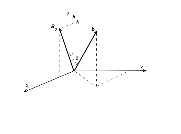
Figure 1: Geometry of the vectors $\mn@boldsymbol{k}$ and $\mn@boldsymbol{b}$ in the coordinate system described in the text. $\mn@boldsymbol{B_{0}}$ is the initial orientation of the magnetic axis.

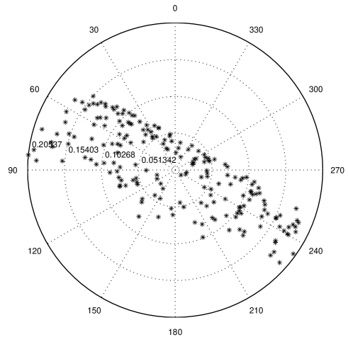
Figure 5: The Lambert’s azimuthal equal area projection of the final Stokes parameters of the sum of modes with the dominant ordinary mode; $\tau\in[0,0.3]$; the role of cyclotron absorption is not negligible, $\eta\in[0.1,0.4]$; $\mu\in[0.1,0.5]$.

It should be noted that the wave mode coupling holds only if the wavevector goes out of the initial plane of magnetic lines. In pulsar case, this condition is certainly satisfied, e.g. because of the magnetosphere rotation. Let us choose the Cartesian coordinate system with the z-axis along the wavevector and the x-axis in the initial plane of magnetic lines (see Fig. 1). The ray is emitted along a field line of the dipolar magnetic field at an angle $\psi$ to the magnetic axis. In the non-rotating magnetosphere, the ray would propagate in the plane of magnetic lines and at distances much larger than the emission altitude would make the angle $\sim\psi$ with the ambient magnetic field because of divergence of the magnetic lines, so that $b_{x}\sim\psi$, $b_{y}=0$. Because of the magnetosphere rotation, $b_{y}$ increases with distance $\propto z/r_{L}$ (the exact formulas for $b_{x}$ and $b_{y}$, which allow for the rotational aberration, are given by the equation (3) in Petrova (2003)). The quantity $\mu\equiv(b_{y}/b_{x})_{r_{p}}\sim r_{p}/(r_{L}\psi)$ is the key parameter which determines the efficiency of wave mode coupling. It should be noted that although as a rule $r_{p}/r_{L}\ll 1$, $\mu$ can be of order unity and even larger. The process of wave mode coupling is most efficient at $\mu=1$, in which case the resultant degree of circular polarization of the waves is as large as about 40% (cf. Fig. 5 in Petrova (2001)). Generally speaking, $\mu$ depends on the geometry of ray propagation and can differ substantially for the rays observed at different pulse longitudes and frequencies as well as for different pulsars. Moreover, $r_{p}$ and $\mu$ may vary from pulse to pulse because of fluctuations in the plasma parameters (cf. equation (3)).

The process of wave mode coupling holds as long as $L_{b}\sim L_{p}$. As the plasma number density decreases further, this process ceases and the waves propagate as in vacuum, preserving their polarization state. For this reason, the wave mode coupling is usually called polarization-limiting effect. However, actually it is the final stage of polarization evolution only if the region of cyclotron resonance lies infinitely far. Otherwise the cyclotron absorption also affects the wave polarization. For the particles with the characteristic Lorentz-factor, the condition of cyclotron resonance, $\omega\gamma\theta^{2}/2=\omega_{H}\equiv\frac{eB}{mc}$, is met at

$$\frac{r_{c}}{r_{L}}=0.55P^{-1}B_{\star 12}^{1/3}\nu_{9}^{-1/3}\gamma_{1.5}^{-1/3}\theta_{-1}^{-2/3}$$ (4)

(e.g. Petrova, 2006). Similarly to the radius of wave mode coupling, the resonance radius is strongly affected by the uncertainty in the angle $\theta$, but generally $r_{c}$ lies within the light cylinder. Comparing the equations (3) and (4), one can conclude that for a wide range of pulsar parameters $r_{c}\sim r_{p}$ and the process of cyclotron absorption can play a marked role in determining the final polarization of radio waves. The quantity $\eta\equiv r_{p}/r_{c}$ is another key parameter of the polarization evolution in pulsar magnetosphere.

Generally speaking, the plasma of pulsar magnetosphere is gyrotropic, i.e. the distribution functions of electrons and positrons are somewhat different. Correspondingly, the natural waves are linearly polarized only in the vicinity of the emission region, where the approximation of infinitely strong magnetic field is still valid. In the outer magnetosphere, in the regions of significant polarization evolution (at $r\sim r_{p},r_{c}$) the natural waves of the medium are generally elliptical. Unfortunately, the question on the net current density and its distribution in the magnetosphere is still open. Given that the electrons and positrons differ only in the number densities and this difference is of the order of the Goldreich-Julian number density, i.e. $\Delta N/N\sim 1/\kappa$, the relative contribution of the plasma gyrotropy to the polarization evolution in the region of wave mode coupling can be estimated as $0.1\kappa_{2}^{-1}\theta_{-1}^{2}\gamma_{1.5}^{2}\omega^{\prime}/\omega_{H}$ (Petrova, 2006); here $\omega^{\prime}$ is the wave frequency in the plasma frame, $\omega^{\prime}\equiv\omega\gamma\theta^{2}/2$. One can see that if the wave mode coupling holds close enough to the region of cyclotron resonance,i.e. if $\omega^{\prime}/\omega_{H}\sim 1$, the contribution of the intrinsic ellipticity of the natural waves can be significant, at least for the rays of a specific geometry. However, as the true form of the net charge density is unknown, we leave out the plasma gyrotropy, keeping in mind that this effect can also be significant and may somewhat alter our quantitative results. In the present paper, we concentrate on studying the evolution of linearly polarized natural waves as a result of propagation effects in pulsar plasma. In our consideration, the wave ellipticity arises and changes purely on account of wave mode coupling and cyclotron absorption. An opposite approach has recently been developed by Luo & Melrose (2004) and Melrose & Luo (2004a), who investigated the characteristics of the elliptically polarized natural waves at $r\sim r_{p}$, ignoring the wave mode coupling in this region. The effect of cyclotron absorption on the elliptical natural waves has been considered in Melrose & Luo (2004b).

An exact treatment of polarization transfer in pulsar plasma with account for the wave mode coupling and cyclotron absorption can be found in Petrova (2006). The evolution of the Stokes parameters of the natural waves is described by the following set of equations:

$$\frac{{\rm d}I}{{\rm d}w}=-\eta^{2}swF_{2}q\left(1-\frac{\mu^{2}}{\eta^{2}w^{2}}\right)-2\mu\eta sF_{2}u\,,$$

$$\frac{{\rm d}q}{{\rm d}w}=-\eta^{2}swF_{2}I\left(1-\frac{\mu^{2}}{\eta^{2}w^{2}}\right)-2\mu\eta sF_{1}v\,,$$

$$\frac{{\rm d}u}{{\rm d}w}=\eta^{2}swF_{1}v\left(1-\frac{\mu^{2}}{\eta^{2}w^{2}}\right)-2\mu\eta sF_{2}I\,,$$

$$\frac{{\rm d}v}{{\rm d}w}=-\eta^{2}swF_{1}u\left(1-\frac{\mu^{2}}{\eta^{2}w^{2}}\right)-2\mu\eta sF_{1}q\,.$$ (5)

Here $w\equiv r_{c}/z$, $s\equiv\frac{1+\mu^{2}}{(1+\mu^{2}/(\eta^{2}w^{2}))^{2}}$,

$$F_{1}\equiv{\rm v.p.}\int\frac{f(\gamma){\rm d}\gamma}{(\gamma/\gamma_{0})^{3}[1-(\gamma/\gamma_{0})^{2}w^{-6}]}\,,$$

$$F_{2}\equiv\frac{\pi}{2}w^{-6}\gamma_{0}f\left[w^{3}\gamma_{0}\right]\,,$$

v.p. means that the integral is taken in the principal value sense, $f(\gamma)$ is the particle distribution function with the normalization $\int f(\gamma){\rm d}\gamma=1$, $\gamma_{0}$ the characteristic Lorentz-factor of the plasma particles, $r_{c}$ the characteristic radius of cyclotron resonance defined as $\omega_{H}(r_{c})\equiv\omega\gamma_{0}\theta^{2}/2$. In equation (5) we have omitted the factors common to all the Stokes parameters, since they are irrelevant to the problem of polarization evolution considered. The set of equations (5) is a generalization of equations (17) in Petrova (2006) for the case of arbitrary $\mu$. At the same time, we still do not include the terms responsible for rotational aberration explicitly and assume that they enter $b_{x}$ and $b_{y}$ as factors of order unity (for more detail see Petrova 2006). The terms containing $F_{1}$ describe polarization evolution because of wave mode coupling, while those containing $F_{2}$ correspond to cyclotron absorption. The initial conditions for the natural waves read: $(I,q,u,v)_{0}=(1,\pm 1,0,0)$, where the upper and lower signs refer to the ordinary and extraordinary waves, respectively.

To proceed further, we choose a simplified distribution function of the plasma particles in the form of a triangle:

$$f(\gamma)=\left\{\begin{array}[]{lr}\frac{\displaystyle\gamma-\gamma_{0}(1-a)}{\displaystyle a^{2}\gamma_{0}^{2}}\,,&\quad\gamma_{0}(1-a)\leq\gamma\leq\gamma_{0}\,,\\ \frac{\displaystyle\gamma_{0}(1+a)-\gamma}{\displaystyle a^{2}\gamma_{0}^{2}}\,,&\quad\gamma_{0}\leq\gamma\leq\gamma_{0}(1+a)\,.\end{array}\right.$$ (6)

Generally speaking, the numerical results on polarization evolution are not very sensitive to the detailed shape of $f(\gamma)$ and are mainly affected by the average Lorentz-factor, $\gamma_{0}$, and the width of the distribution (the parameter $a$ in equation (6)). The set of equations (5) along with equation (6) describe polarization evolution of the original natural waves in the hot magentized weakly inhomogeneous plasma of pulsars.

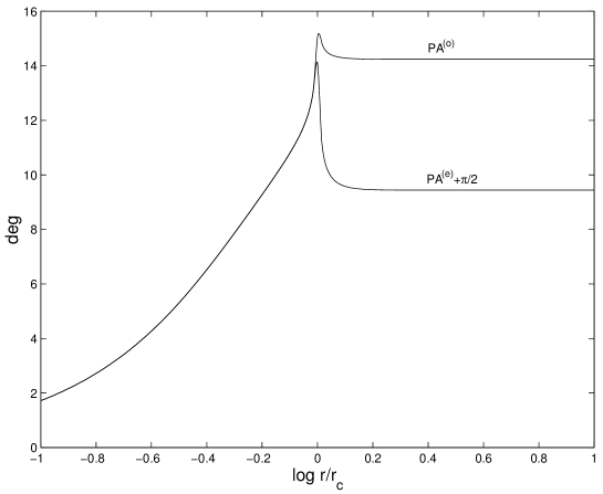
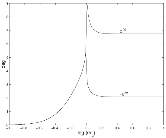
Figure 2: Position angle (a) and ellipticity (b) of the original ordinary and extraordinary modes as functions of distance in pulsar magnetosphere; $\mu=0.3$, $\eta=1$, $a=0.1$.

Since the natural waves are completely polarized by definition, their polarization state is described by two independent quantities, e.g. PA, $\psi\equiv 0.5\arctan(u/q)$, and the ellipticity, $\chi\equiv 0.5\arctan\frac{v}{\sqrt{q^{2}+u^{2}}}$. Figure 2 shows an example of numerical tracings of $\psi$ and $\chi$ of the original ordinary and extraordinary waves as they propagate in pulsar magnetosphere. One can see that polarization evolution can indeed be significant and differs markedly for the two modes.

3 Statistics of the final polarization parameters

3.1 Histograms of PA and ellipticity

As is discussed above, polarization evolution is determined by the parameters $\mu$ and $\eta$ and is affected by the parameters of the particle distribution function. For the rays observed at a fixed pulse longitude, the locations of the regions of wave mode coupling and cyclotron resonance may vary from pulse to pulse because of fluctuations in the number density and the characteristic Lorentz-factor of the plasma particles. Besides that, the fluctuations in the plasma distribution may affect refraction of the waves, so that the rays of a certain orientation may follow somewhat different trajectories in the open field line tube. All this is believed to influence the final polarization states of the original natural waves. Note that although the modern theories of the pulsar pair creation cascade say nothing about the fluctuations in the resultant distribution of the secondary plasma, an idea of such fluctuations is supported by the random nature of the cascade process and is strongly suggested by the variability of the observed individual pulse profiles.

In the upper panel of Fig. 2, the left plot shows the histogram of the final PA of the original natural waves in case of randomly varying parameters $\mu$ and $\eta$. One can see that the peaks are separated by not exactly $90^{\circ}$, the scatter of PA values around the peaks is about $10^{\circ}$ and the ordinary mode (that with positive PA) shows somewhat less scatter than the extraordinary one. The histogram of mode ellipticities for the same $\mu$ and $\eta$ is shown in the right plot of the upper panel in Fig. 2. Note that the peaks are not symmetrical with respect to zero and the extraordinary mode exhibits a more pronounced scatter.

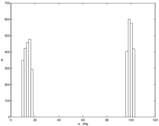
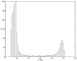
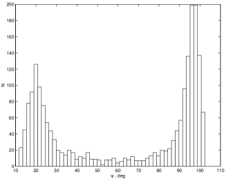
Figure 3: Numerically simulated histograms of the final PA and ellipticity after polarization evolution in the fluctuating plasma. The parameters $\mu$ and $\eta$ are uniformly distributed over the intervals [0.2,0.4] and [0.9,1.1], respectively. The upper panel shows the histograms for the original ordinary and extraordinary modes. The middle and bottom panels correspond to the sum of modes with random intensity ratio. The coefficient of conversion is uniformly distributed in the intervals [0,1] and [0.6,1], respectively.

The middle and bottom panels of Fig. 3 show the histograms of PA and ellipticity for the sum of the two polarization modes given random variations in $\mu$, $\eta$ and the mode intensity ratio. In the present consideration, we assume that initially only the ordinary mode is emitted, whereas the extraordinary one arises as a result of partial conversion of the ordinary mode deep inside the magnetosphere (see Petrova, 2001). This is supported by the recently discovered anticorrelation of the mode intensities (Edwards & Stappers, 2004). Since the mode conversion is a propagation effect, its efficiency is also determined by the instantaneous distribution of the plasma and is believed to fluctuate. Thus, the coefficient of conversion, $\tau$, is considered as a random quantity. Generally speaking, it may be correlated with $\mu$ and $\eta$, but as the process of mode conversion takes place far from $r_{p}$ and $r_{c}$, the correlation is thought to be weak and is neglected throughout the paper. In the middle panel of Fig. 2, $\tau$ is taken to be distributed over the whole interval from 0 to 1, whereas in the bottom panel $\tau\in[0.6,1]$.

Although in the former case the probability to dominate is the same for the two types of original natural waves, the humps at the PA histograms are substantially distinct: the peak corresponding to the ordinary waves is much more pronounced. This is a consequence of cyclotron absorption, which suppresses the extraordinary constituent of the wave polarization stronger. The extraordinary-mode hump looks more smeared and is connected to the ordinary-mode one with a bridge. In the bottom panel, the humps change in dominance, but the ordinary mode is still present, despite complete dominance of the extraordinary waves just after conversion. This is again because of differential action of cyclotron absorption on the two types of natural waves. The bridge between the humps looks more pronounced, and the histogram on the whole is similar to the observed ones (e.g. McKinnon, 2003).

In the middle histogram of the ellipticity, the hump corresponding to the extraordinary mode is barely resolved, whereas the ordinary mode peaks at $\chi\approx 0$. On the whole, this distribution looks like a unimodal one with a long tail. As can be seen in the bottom histogram of $\chi$, only positive values are met and the two humps are barely resolved. This distribution can also be regarded as a unimodal one, in contrast to the corresponding histogram of PA. It is not our aim here to fit the concrete distributions observed, but Fig. 3 demonstrates the principal possibility of such fits within the framework of the propagation model of pulsar polarization.

3.2 Two-dimensional scatter-plots

Propagation origin of pulsar polarization implies a certain correlation between the mode ellipticity and PA: Both these quantities are determined by the instantaneous state of the plasma and vary from pulse to pulse because of fluctuations in the plasma flow. Now we are going to model the observational signatures of this correlation for different sets of $\mu$ and $\eta$ and compare our simulations with the observational results.

At a fixed pulse longitude, the simulated individual-pulse polarization presents a sum of the two polarization modes with random intensity ratio. The resultant Stokes parameters are plotted in the Lambert’s azimuthal equal area projection, as is done by observers (Edwards & Stappers, 2004; Edwards, 2004). As each mode can dominate from time to time, at the Poincaré sphere the resultant Stokes vectors tend to group around the roughly orthogonal locations corresponding to the observed modes. Let us choose the spherical coordinate system with the polar axis along the fiducial vector of the normalized Stokes parameters, ${\mn@boldsymbol{s}}_{p}=\{q_{p},u_{p},v_{p}\}$, $q_{p}^{2}+u_{p}^{2}+v_{p}^{2}=1$, which is the average over the Stokes vectors belonging to one of the observed modes. The quantities $\rho$ and $\lambda$ are the polar angle and azimuth of the normalized individual Stokes vectors (q,u,v) in this spherical system:

$$\rho=\arccos(qq_{p}+uu_{p}+vv_{p})\,,$$

$$\lambda=\arctan\left[\frac{uq_{p}-qu_{p}}{(qq_{p}+uu_{p})v_{p}-v(q_{p}^{2}+u_{p}^{2})}\right]\,.$$ (7)

If one consider $\rho$ and $\lambda$ as the polar coordinates (the radius and azimuth, respectively), we come to the Lambert’s azimuthal equal area projection of the Poincaré sphere. This projection is interrupted at the equator, and for the Stokes vectors lying in the southern hemisphere (i.e. for the second mode) the projection of the sphere with the polar axis along ${\mn@boldsymbol{s}}_{m}=-{\mn@boldsymbol{s}}_{p}$ is considered (for more detail see Edwards & Stappers, 2004).

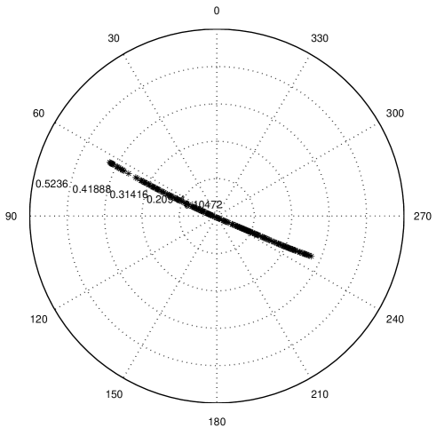
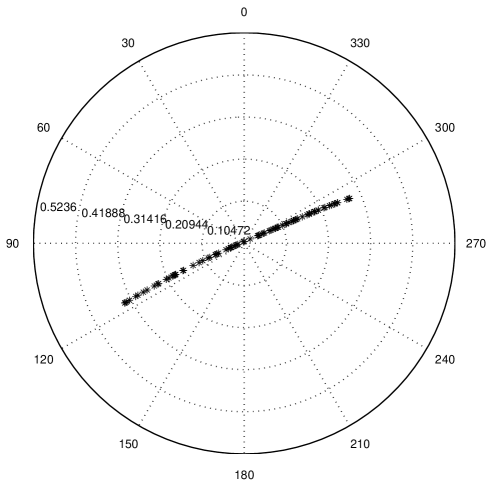
Figure 4: Two-dimensional scatter plots of the final Stokes parameters of the original ordinary (left panel) and extraordinary (right panel) modes in the Lambert’s azimuthal equal area projection (for more detail see text); $\mu\in[0.1,0.5]$ and $\eta\in[0.01,0.05]$. The one-to-one correspondence of the polarization parameters is evident.

Figure 4 shows the two-dimensional plots for the two original natural modes after their evolution in the plasma in case of negligible cyclotron absorption, $\eta\sim 0.01$, and moderate mode coupling, $\mu\sim 0.1$. Here ${\mn@boldsymbol{s}}_{p}$ corresponds to the original ordinary mode. One can see that the process of mode coupling in the fluctuating plasma results in the unambiguous relation of the polarization characteristics, which has already been proposed as a basis for diagnostics of pulsar plasma (Petrova, 2003). At these plots, the points prefer certain azimuths, which is in qualitative agreement with the observational result of Edwards (2004) (see Fig. 5 there), though the scatter of the observational points is enormously large. Note that this scatter cannot be reproduced by considering the sum of the two modes with random intensities. Introducing a slight non-orthogonality of the modes because of cyclotron absorption ($\eta\sim 0.1$) makes the plot more realistic (see Fig. 5 for the case of completely dominating original ordinary mode, $\tau\in[0,0.3]$), though the scatter of the points is still insufficient.

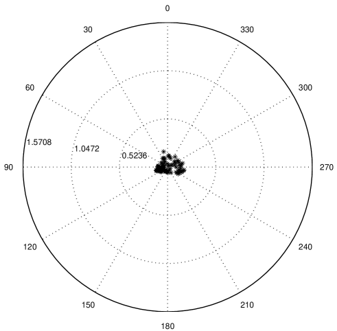
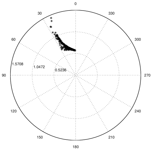
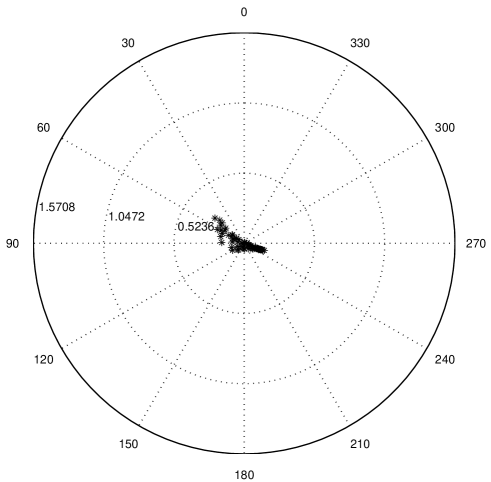
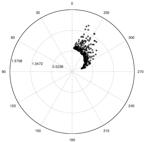
Figure 6: Two-dimensional scatter plots of the final Stokes parameters in case of strong non-orthogonality of the modes, $\eta\in[0.5,1.5]$. In the upper and lower panels, $\tau\in[0.5,1]$ and $\tau\in[0,1]$, respectively, and ${\mn@boldsymbol{s}}_{p}$ is centered on the ordinary- and extraordinary-wave positions, correspondingly.

Figure 6 shows the two-dimensional scatter plots in case of strong non-orthogonality of the modes ($\eta\sim 1$). In the upper panel, the fiducial Stokes vector, ${\mn@boldsymbol{s}}_{p}$, corresponds to the state with the dominant ordinary mode, whereas the coefficient of conversion is uniformly distributed in the interval $[0.5,1]$. Note that although in this case the conversion of the ordinary waves into the extraordinary ones is efficient, the final polarization state of the sum of the modes can still be close to that of the ordinary ones because of less significant absorption of the ordinary waves and because of a marked non-orthogonality of the modes. The bottom panel of Fig. 6 corresponds to the case of a uniform distribution of $\tau$ over the whole interval from 0 to 1, with ${\mn@boldsymbol{s}}_{p}$ directed along the extraordinary mode vector. The plots in both panels exhibit strong non-orthogonality of polarization states, with the secondary modes forming the characteristic arc-like features, which are in a qualitative agreement with those discovered in observations (cf. Fig. 2 in Edwards & Stappers, 2004). Note, however, that the scatter of the simulated points and the degree of non-orthogonality are substantially less than those in the observational plots. This may be an indication of the role of some additional effects in the formation of the single-pulse polarization of pulsars.

4 Discussion and conclusions

The hot magnetized weakly inhomogeneous plasma of pulsars may substantially affect the radio wave propagation. The polarization states of the original natural waves may change markedly because of the wave mode coupling and cyclotron absorption. The former process turns the original linearly polarized waves into the elliptical ones, which are still purely orthogonal at the Poincaré sphere. The mode coupling efficiency is determined by the location of the coupling region, $r_{p}$, in the tube of open magnetic lines. The role of cyclotron absorption in the evolution of wave polarization depends on how close the regions of mode coupling and cyclotron resonance are, being most prominent in case of their approximate coincidence, $\eta=r_{p}/r_{c}\approx 1$. Typically $r_{c}$ lies beyond $r_{p}$, in which case cyclotron absorption leads to the non-orthogonality of the waves. Note that all the way in the magnetosphere the original natural waves remain completely polarized.

Temporal fluctuations in the plasma flow are believed to underlie the fluctuations of the individual pulse polarization. The plasma distribution in the open field line tube can be strongly variable because of the random character of the pair creation process. Hence, for the rays observed at a fixed pulse longitude, both $r_{p}$ and $r_{c}$ can change from pulse to pulse due to variations of the number density and characteristic Lorentz-factor of the plasma. Besides that, the variations of the plasma distribution may affect refraction of waves, so that the rays observed at a given pulse longitude may follow somewhat different trajectories in the magnetosphere and have different tilts to the ambient magnetic field while passing through the regions of mode coupling and cyclotron resonance.

The intensity ratio of the modes fluctuates as well, and it is also thought to result from the plasma fluctuations in the magnetosphere. The point is that the extraordinary natural waves have vacuum dispersion and can hardly be generated directly by any conceivable emission process in the plasma. Therefore they are likely to originate as a result of partial conversion of the ordinary waves, which can take place in the regions of quasi-longitudinal propagation deep inside the magnetosphere (Petrova, 2001). The idea of mode conversion is supported by the recently discovered anticorrelation of the mode intensities (Edwards & Stappers, 2004). In the framework of this view, the mode intensity ratio is determined by the coefficient of conversion and changes from pulse to pulse because of fluctuations in the plasma flow.

Thus, the propagation model of pulsar polarization incorporates two superposed completely polarized modes with randomly varying polarization states and intensities. It is important to note that because of cyclotron absorption the superposed modes can become non-orthogonal, whereas the original natural waves are purely orthogonal by definition.

In the present paper, the statistics of the individual pulse polarization have been simulated under the assumption that the parameters $\mu$ and $\eta$ as well as the coefficient of conversion, $\tau$, are the random quantities with unifirm distributions over some intervals. The resultant histograms of PA exhibit two humps markedly smeared and connected with a bridge. The peaks can be separated by not exactly $90^{\circ}$. The histograms of the resultant ellipticity look like the unimodal ones because of a very small separation between the peaks of the two observational modes. Furthermore, it may happen that in the whole sample the ellipticity is purely of one sign, whereas the corresponding histogram of PA is bimodal. Although direct fits to the observational data are beyond the scope of the present paper, our results confirm the ability of the propagation model to account for the main features of the observed histograms of PA and ellipticity.

Propagation origin of pulsar polarization implies a certain correlation between the mode ellipticity and PA. Given that the contribution of cyclotron absorption is negligible and the final polarization is determined solely by the mode coupling, there is a one-to-one correspondence between the mode ellipticity and PA. However, it is not proved by the observational data available. Although an evidence for the expected relation is indeed present in the polarization of PSR B0818-13 (Edwards, 2004), the scatter of the observational points appears dramatic, and it cannot be reproduced by taking into account the fluctuations of the mode intensity ratio. In case of moderately weak cyclotron absorption, a slight non-orthogonality of the fluctuating modes causes an additional scatter of the polarization parameters and allows to reproduce the observational plots on a qualitative level, though the scatter is still insufficient quantitatively. In case of strong non-orthogonality of the modes, our model qualitatively reproduces the characteristic arc-like features present in the observational plots for PSR B0329+54 (Edwards & Stappers, 2004), though the magnitude of non-orthogonality and the total scatter of the simulated points are again less than in observations.

Thus, on a qualitative level, the expected correlations of polarization parameters are compatible with the observational data. This is a strong argument in favour of the propagation model of pulsar polarization. Apparently, to achieve better quantitative agreement with the observational results it is necessary to improve and further develop the model suggested. In the present consideration, we have ignored the net charge density in the magnetosphere and treated the process of cyclotron absorption in the limit of small pitch-angles of the particles. In reality, both these assumptions can be violated, so that our results on the individual-pulse polarization and its statistics can be somewhat modified. Besides that, pulsar emission can be considered as a sum of contributions from multiple subsources (e.g. Gil & Lyne, 1995; Melrose et al., 2006), in which case the possibilities of modeling the resultant polarization are much wider.

In conclusion, it should be pointed out that the model suggested allows a unique possibility of diagnostics of pulsar plasma by means of the individual-pulse polarization.

References

- Edwards (2004) Edwards R., 2004, A&A, 426, 677
- Edwards & Stappers (2004) Edwards R., Stappers B., 2004, A&A, 421, 681
- Gil et al. (1991) Gil J. A., Snakowski J. K., Stinebring D. R., 1991, A&A, 242, 119
- Gil et al. (1992) Gil J. A., Lyne A. G., Rankin J. M., Snakowski J. K., Stinebring D.R., 1992, A&A, 255, 181
- Gil & Lyne (1995) Gil J. A., Lyne A. G., 1995, MNRAS, 276, L55
- Karastergiou et al. (2001) Karastergiou A., von Hoensbroech A., Kramer M. et al., 2001, A&A, 379, 270
- (7) Karastergiou A., Johnston S., Kramer M., 2003, A&A, 404, 325
- Luo & Melrose (2004) Luo Q., Melrose D.B., 2004, in: F. Camilo & B.M. Gaensler (eds.) Young Neutron Stars and Their Environments, IAU Symposium, Vol. 218 (San Francisco:ASP), 381
- Lyubarskii & Petrova (1998) Lyubarskii Yu.E., Petrova S.A., 1998, A&A, 337, 433
- Lyubarskii & Petrova (1999) Lyubarskii Yu.E., Petrova S.A., 1999, Ap&SS, 262, 379
- McKinnon (2003) McKinnon M.M., 2003, ApJ, 590, 1026
- McKinnon & Stinebring (1998) McKinnon M.M., Stinebring D.R., 1998, ApJ, 502, 883
- McKinnon & Stinebring (2000) McKinnon M.M., Stinebring D.R., 2000, ApJ, 529, 435
- Melrose & Luo (2004a) Melrose D.B., Luo Q., 2004a, MNRAS, 352, 915
- Melrose & Luo (2004b) Melrose D.B., Luo Q., 2004b, Phys. Rev. E 70, 016404
- Melrose et al. (2006) Melrose D., Miller A., Karastergiou A., Luo Q., 2006, MNRAS, 365, 638
- Petrova (2001) Petrova S.A., 2001, A&A, 378, 883
- Petrova (2002) Petrova S.A., 2002, MNRAS, 336, 774
- Petrova (2003) Petrova S.A., 2003, A&A, 408, 1057
- Petrova (2005) Petrova S.A., 2005, in: ”Astrophysical Sources of High-Energy Particles and Radiation”, Eds. T.Bulik, B.Rudak and G.Madejski, AIP Conf. Proceedings, v.801, p.286
- Petrova (2006) Petrova S.A., 2006, MNRAS, in press
- Petrova & Lyubarskii (2000) Petrova S.A., Lyubarskii Yu.E., 2000, A&A, 355, 1168
- Radhakrishnan & Cooke (1969) Radhakrishnan V., Cooke D.J., 1969, ApJLet, 3, 225