A TOY MODEL FOR MAGNETIC CONNECTION IN BLACK-HOLE ACCRETION DISC

Abstract

A toy model for magnetic connection in black hole (BH) accretion disc is discussed based on a poloidal magnetic field generated by a single electric current flowing around a Kerr black hole in the equatorial plane. We discuss the effects of the coexistence of two kinds of magnetic connection (MC) arising respectively from (1) the closed field lines connecting the BH horizon with the disc (henceforth MCHD), and (2) the closed field lines connecting the plunging region with the disc (henceforth MCPD). The magnetic field configuration is constrained by conservation of magnetic flux and a criterion of the screw instability of the magnetic field. Two parameters $\lambda$ and $\alpha_{m}$ are introduced to describe our model instead of resolving the complicated MHD equations. Compared with MCHD, energy and angular momentum of the plunging particles are extracted via MCPD more effectively, provided that the BH spin is not very high. It turns out that negative energy can be delivered to the BH by the plunging particles without violating the second law of BH thermodynamics, however it cannot be realized via MCPD in a stable way.

1 INTRODUCTION

Recently, much attention has been paid to the magnetic connection (MC) of a rotating black hole (BH) with its surrounding accretion disc (Blandford 1999; Li 2000a; Wang, Xiao & Lei 2002, Wang et al. 2003, hereafter W02 and W03, respectively). The MC process can be regarded as one of the variants of the Blandford-Znajek (BZ) process proposed near three decades ago (Blandford & Znajek 1977), which involves the closed magnetic field lines connecting a BH with its surrounding disc. This mechanism has been used to explain a very steep emissivity in the inner region of the disc, which is consistent with the XMM-Newton observation of the nearby bright Seyfert1 galaxy MCG-6-30-15 (Wilms 2001; Li 2002a; W03).

Blandford (2002) described several electromagnetic ways to extract the rotational energy associated with a spinning BH, in which the MC between the plunging region and the disc (hereafter MCPD) is included. However, MCPD has not been discussed in detail in the previous work, and the origin of these magnetic field configurations remains unclear.

Recently, Li (2002b, hereafter L02) discussed the MC between the BH horizon and the disc (hereafter MCHD) by assuming a toroidal electric current $I$ flowing on a circle of $r={r}^{\prime}$ in the equatorial plane of a Kerr BH, i.e.,

$$J^{a}=\frac{I}{r}\left({\Delta\mathord{\left/{\vphantom{\Delta A}}\right.\kern-1.2pt}A}\right)^{1/2}\left({\partial\mathord{\left/{\vphantom{\partial{\partial\phi}}}\right.\kern-1.2pt}{\partial\phi}}\right)^{a}\delta(r-{r}^{\prime})\delta(\cos\theta).$$ (1)

The metric around a Kerr BH is given in Boyer-Lindquist coordinates (MacDonald and Thorne 1982, hereafter MT82)

$$\begin{array}[]{l}ds^{2}=-\left({1-\frac{2Mr}{\rho^{2}}}\right)dt^{2}\\ \quad\quad-\frac{4aMr\sin^{2}\theta}{\rho^{2}}dtd\varphi+\frac{\rho^{2}}{\Delta}dr^{2}\mbox{ + }\rho^{2}d\theta^{2}+\frac{A\sin^{2}\theta}{\rho^{2}}d\varphi^{2},\end{array}$$ (2)

where the concerned Kerr metric parameters are defined as

$$\left\{{\begin{array}[]{l}A=\left({r^{2}+a^{2}}\right)^{2}-a^{2}\Delta\sin^{2}\theta,\mbox{ }\rho^{2}=r^{2}+a^{2}\cos^{2}\theta,\mbox{ }\\ \Delta=r^{2}+a^{2}-2Mr,\mbox{ }\varpi=\left({A\mathord{\left/{\vphantom{A{\rho^{2}}}}\right.\kern-1.2pt}{\rho^{2}}}\right)^{1\mathord{\left/{\vphantom{12}}\right.\kern-1.2pt}2}\sin\theta,\\ \alpha=\left({{\rho^{2}\Delta}\mathord{\left/{\vphantom{{\rho^{2}\Delta}A}}\right.\kern-1.2pt}A}\right)^{1\mathord{\left/{\vphantom{12}}\right.\kern-1.2pt}2},\quad\omega=2aMr/A\\ \end{array}}\right.$$ (3)

In equation (3) $a$ is the specific angular momentum of the BH, which is related to the BH mass $M$, angular momentum $J$ and spin $a_{*}$ by $a\equiv J\mathord{\left/{\vphantom{JM}}\right.\kern-1.2pt}M=a_{*}M$.

Not long ago, Li (2000b, hereafter L00) discussed a scenario of extracting energy from a Kerr BH through the plunging region, where the open magnetic field lines connect plasma particles with remote loads. It is argued in L00 that the energy extracted from the particles can be so large that the particles have negative energy as they fall into the BH, if the magnetic field is strong enough.

Motivated by the above works, we propose a scenario of extracting energy from a Kerr BH based on the magnetic field configuration arising from a toroidal electric current $I$ flowing at the innermost stable circular orbit (ISCO). The magnetic field configuration contains both MCHD and MCPD, being constrained by the conservation of magnetic flux and a criterion of the screw instability of the magnetic field. It is shown that MCPD is more important than MCHD in transferring energy and angular momentum to the disc for low BH spins. It turns out that negative energy can be delivered to the BH by the plunging particles without violating the second law of BH thermodynamics, however it cannot be realized via MCPD in a stable way.

This paper is organized as follows. In $\S$ 2 we present a description of our model, in which MCHD and MCPD coexist in a large-scale magnetic field generated by a toroidal electric current flowing at ISCO. In $\S$ 3 we calculate and compare the powers and torques in MCHD and MCPD. In $\S$ 4 the condition of negative energy of plunging particles is studied in based on some reasonable constraints: (i) a positive accretion rate, (ii) an increasing BH entropy, (iii) a stationary accretion and (iv) a stable energy extraction for the plunging particles. In $\S$ 5 we compare the efficiencies of releasing energy arising from disc accretion, MCHD and MCPD. Finally, in $\S$ 6, we summarize our main results, and discuss some issues related to our model. Throughout this paper the geometric units $G=c=1$ are used.

2 DESCRIPTION OF OUR MODEL

2.1 Magnetic field configuration produced by a toroidal current

It is assumed that the magnetic field in the neighborhood of the BH and its surrounding disc is ideally conducting and force-free, and the magnetic field, electric field and other quantities are measured by zero-angular-momentum observers defined by Bardeen, Press & Teukolsky (1972). The magnetic field configuration produced by a toroidal current flowing at the inner edge of the disc as shown in Figure 1, which contains both MCHD and MCPD. In this paper we assume that the toroidal current flows at ISCO, being represented by the symbol “$\otimes$”. The quantities $r_{H}$ and $r_{ms}$ are respectively the radii of the BH horizon and ISCO, and they read (Novikov & Thorne 1973)

$$r_{{}_{H}}=M\left({1+\sqrt{1-a_{*}^{2}}}\right),$$ (4)

$$\left\{{\begin{array}[]{l}r_{ms}\equiv M\chi_{ms}^{2},\\ \chi_{ms}=\left\{{3+A_{2}\pm\left[{\left({3-A_{1}}\right)\left({3+A_{1}+2A_{2}}\right)}\right]^{1/2}}\right\}^{1/2},\mbox{ }\\ A_{1}=1+\left({1-a_{*}^{2}}\right)^{1/3}\left[{\left({1+a_{*}}\right)^{1/3}+\left({1-a_{*}}\right)^{1/3}}\right],\\ A_{2}=\left({3a_{*}^{2}+A_{1}^{2}}\right)^{1/2}.\\ \end{array}}\right.$$ (5)

The quantity $r_{e}$ is the radius of the infinite redshift surface and it reads

$$r_{e}\left(\theta\right)=M\left({1+\sqrt{1-a_{*}^{2}\cos^{2}\theta}}\right).$$ (6)

Figure 1: Magnetic field configuration corresponding to MCHD and MCPD, where the symbol “$\otimes$” represents a toroidal current at the inner edge of the disc.

The radius $r_{e}$ increases with the polar angle $\theta$, attaining its maximum at the equatorial plane, i.e., $r_{e}\left({\pi\mathord{\left/{\vphantom{\pi 2}}\right.\kern-1.2pt}2}\right)=2M$. The range of the ergosphere is given by

$${r}_{{}_{H}}<r<r_{e}\left(\theta\right),$$ (7)

and the range of the plunging region is

$${r}_{{}_{H}}<r<r_{ms}.$$ (8)

The magnetic flux through a surface bounded by a circle with $r=$const and $\theta=$const is

$$\Psi\left({r,\theta;{r}^{\prime}}\right)=2\pi A_{\phi}\left({r,\theta;{r}^{\prime}}\right),$$ (9)

where $A_{\phi}$ is the toroidal component of the vector potential produced by the toroidal electric current $I$ at $r={r}^{\prime}$ in the equatorial plane of the Kerr BH. Defining $\tilde{r}\equiv r\mathord{\left/{\vphantom{rM}}\right.\kern-1.2pt}M$ and $B_{0}\equiv{2I}\mathord{\left/{\vphantom{{2I}M}}\right.\kern-1.2pt}M$, we have $\Psi\propto A_{\varphi}\propto MI={B_{0}M^{2}}\mathord{\left/{\vphantom{{B_{0}M^{2}}2}}\right.\kern-1.2pt}2$ and

$$\tilde{\Psi}\left({\tilde{r},\theta;\tilde{{r}^{\prime}}}\right)={2\pi A_{\varphi}\left({r,\theta;{r}^{\prime}}\right)}\mathord{\left/{\vphantom{{2\pi A_{\varphi}\left({r,\theta;{r}^{\prime}}\right)}{\left({B_{0}M^{2}}\right)}}}\right.\kern-1.2pt}{\left({B_{0}M^{2}}\right)}.$$ (10)

Equation (10) provides a mapping relation between any two circles $\left({\tilde{r}_{1},\theta_{1}}\right)$ and $\left({\tilde{r}_{2},\theta_{2}}\right)$ embedded in the same magnetic surface as follows,

$$\tilde{\Psi}\left({\tilde{r}_{1},\theta_{1};\tilde{{r}^{\prime}}}\right)=\tilde{\Psi}\left({\tilde{r}_{2},\theta_{2};\tilde{{r}^{\prime}}}\right).$$ (11)

Znajek (1978) and Linet (1979) derived the relation between the vector potential $A_{\varphi}\left({r,\theta;{r}^{\prime}}\right)$ and the current $I$ as follows.

$$\begin{array}[]{l}A_{\varphi}=2\sum\limits_{l=1}^{\infty}\{{{\alpha_{l}^{r}\left[{ra\sin^{2}\theta\frac{\Delta}{\rho^{2}}F_{1}-a\sin^{2}\theta\cos\theta F_{2}}\right]}}\\ \quad\quad+\alpha_{l}^{i}\left[-a^{2}\sin^{2}\theta\cos\theta\frac{\Delta}{\rho^{2}}F_{1}-r\sin^{2}\theta F_{2}+\frac{\Delta\sin^{2}\theta}{l\left({l+1}\right)}F_{3}\right]\}\\ \quad\quad+2\sum\limits_{l=1}^{\infty}\{{{\beta_{l}^{r}\left[{ra\sin^{2}\theta\frac{\Delta}{\rho^{2}}F_{4}-a\sin^{2}\theta\cos\theta F_{5}}\right]}}\\ \quad\quad+\beta_{l}^{i}\left[{-a^{2}\sin^{2}\theta\cos\theta\frac{\Delta}{\rho^{2}}F_{4}}-r\sin^{2}\theta F_{5}+\frac{\Delta\sin^{2}\theta}{l\left({l+1}\right)}F_{6}\right]\}\end{array}$$ (12)

where in equation (12) the functions $F_{1}$ — $F_{6}$ are defined by

$$\left\{{\begin{array}[]{l}F_{1}\equiv\frac{1}{\sqrt{M^{2}-a^{2}}}{P}^{\prime}_{l}\left(u\right)P_{l}\left({\cos\theta}\right),\\ F_{2}\equiv\frac{r^{2}+a^{2}}{\rho^{2}}P_{l}\left(u\right){P}^{\prime}_{l}\left({\cos\theta}\right)\mbox{,}\\ F_{3}\equiv\frac{1}{\sqrt{M^{2}-a^{2}}}{P}^{\prime}_{l}\left(u\right){P}^{\prime}_{l}\left({\cos\theta}\right),\\ F_{4}\equiv\frac{1}{\sqrt{M^{2}-a^{2}}}{Q}^{\prime}_{l}\left(u\right)Q_{l}\left({\cos\theta}\right),\\ F_{5}\equiv\frac{r^{2}+a^{2}}{\rho^{2}}Q_{l}\left(u\right){Q}^{\prime}_{l}\left({\cos\theta}\right)\\ F_{6}\equiv\frac{1}{\sqrt{M^{2}-a^{2}}}{Q}^{\prime}_{l}\left(u\right){Q}^{\prime}_{l}\left({\cos\theta}\right)\mbox{. }\\ \end{array}}\right.$$ (13)

In equation (13) we have $u\equiv{\left({r-M}\right)}\mathord{\left/{\vphantom{{\left({r-M}\right)}{\sqrt{M^{2}-a^{2}}}}}\right.\kern-1.2pt}{\sqrt{M^{2}-a^{2}}}$, $P_{l}\left(z\right)$ and $Q_{l}\left(z\right)$ are Legendre functions with ${P}^{\prime}_{l}\left(z\right)\equiv{dP_{l}\left(z\right)}\mathord{\left/{\vphantom{{dP_{l}\left(z\right)}{dz}}}\right.\kern-1.2pt}{dz}$ and ${Q}^{\prime}_{l}\left(z\right)\equiv{dQ_{l}\left(z\right)}\mathord{\left/{\vphantom{{dQ_{l}\left(z\right)}{dz}}}\right.\kern-1.2pt}{dz}$. The coefficients $\alpha_{l}^{r}$, $\alpha_{l}^{i}$, $\beta_{l}^{r}$ and $\beta_{l}^{i}$ are defined as follows:

(1) for $r<{r}^{\prime}$, $\beta_{l}^{r}=\beta_{l}^{i}=0$ for all $l$; but

$$\alpha_{l}^{r}\equiv\frac{\pi\left({2l+1}\right)I}{l\left({l+1}\right)\left({M^{2}-a^{2}}\right)}\left({\frac{{\Delta}^{\prime}}{{A}^{\prime}}}\right)^{1\mathord{\left/{\vphantom{12}}\right.\kern-1.2pt}2}{\Delta}^{\prime}aP_{l}\left(0\right){Q}^{\prime}_{l}\left({u}^{\prime}\right),$$ (14)

$$\begin{array}[]{l}\alpha_{l}^{i}\equiv\frac{\pi\left({2l+1}\right)I}{l\left({l+1}\right)\left({M^{2}-a^{2}}\right)}\left({\frac{{\Delta}^{\prime}}{{A}^{\prime}}}\right)^{1\mathord{\left/{\vphantom{12}}\right.\kern-1.2pt}2}\\ \quad\quad\times[{-\left({{r}^{\prime 2}+a^{2}}\right){P}^{\prime}_{l}\left(0\right)Q_{l}\left({u}^{\prime}\right)}\\ \quad\quad+\frac{{r}^{\prime}{\Delta}^{\prime}}{l\left({l+1}\right)}\frac{1}{\sqrt{M^{2}-a^{2}}}{P}^{\prime}_{l}\left(0\right){Q}^{\prime}_{l}\left({u}^{\prime}\right)];\\ \end{array}$$ (15)

(2) for $r>{r}^{\prime}$, $\alpha_{l}^{r}=\alpha_{l}^{i}=0$ for all $l$; but

$$\beta_{l}^{r}\equiv\frac{\pi\left({2l+1}\right)I}{l\left({l+1}\right)\left({M^{2}-a^{2}}\right)}\left({\frac{{\Delta}^{\prime}}{{A}^{\prime}}}\right)^{1\mathord{\left/{\vphantom{12}}\right.\kern-1.2pt}2}{\Delta}^{\prime}aP_{l}\left(0\right){P}^{\prime}_{l}\left({u}^{\prime}\right),$$ (16)

$$\begin{array}[]{l}\beta_{l}^{i}\equiv\frac{\pi\left({2l+1}\right)I}{l\left({l+1}\right)\left({M^{2}-a^{2}}\right)}\left({\frac{{\Delta}^{\prime}}{{A}^{\prime}}}\right)^{1\mathord{\left/{\vphantom{12}}\right.\kern-1.2pt}2}\\ \quad\quad\times[{-\left({{r}^{\prime 2}+a^{2}}\right){P}^{\prime}_{l}\left(0\right)P_{l}\left({u}^{\prime}\right)}\\ \quad\quad+\frac{{r}^{\prime}{\Delta}^{\prime}}{l\left({l+1}\right)}\frac{1}{\sqrt{M^{2}-a^{2}}}{P}^{\prime}_{l}\left(0\right){P}^{\prime}_{l}\left({u}^{\prime}\right)],\\ \end{array}$$ (17)

where in equations (14)—(17) we have ${\Delta}^{\prime}\equiv\Delta\left({r={r}^{\prime}}\right)$ and ${A}^{\prime}\equiv A\left({r={r}^{\prime},\mbox{ }\theta=\pi\mathord{\left/{\vphantom{\pi 2}}\right.\kern-1.2pt}2}\right)$.

2.2 Mapping relations for MCHD and MCPD

For the toroidal current located at $r_{ms}$ the mapping relation between the circle at the BH horizon with the longitudinal angle $\theta$ and the circle at the thin disc with the radius $r$ can be written as

$$\tilde{\Psi}\left({\tilde{r},\pi\mathord{\left/{\vphantom{\pi 2}}\right.\kern-1.2pt}2;\tilde{r}_{ms}}\right)=\tilde{\Psi}\left({\tilde{r}_{{}_{H}},\theta;\tilde{r}_{ms}}\right).$$ (18)

It is assumed that the toroidal current located at $r_{ms}$ has a very small circular section of radius ${r}^{\prime}_{\varepsilon}=\varepsilon r_{ms}$, so that the poloidal magnetic field is proportional to the radius ${r}^{\prime}$ for $0<{r}^{\prime}<{r}^{\prime}_{\varepsilon}$. In this way the infinite magnetic field is avoided as $r$close to $r_{ms}$, keeping magnetic field configuration outside ${r}^{\prime}_{\varepsilon}$ unchanged. In this paper we take $\varepsilon=10^{-4}$ in calculations (The influence of the choice of $\varepsilon$ is discussed in $\S$ 6).

The innermost magnetic surface for MCHD is defined as a surface connecting the horizon at $\theta=\pi\mathord{\left/{\vphantom{\pi 2}}\right.\kern-1.2pt}2$ with the disc at $\tilde{r}_{0}\geq\tilde{r}_{ms}$, and it can be determined by

$$\tilde{\Psi}\left({\tilde{r}_{0},\pi\mathord{\left/{\vphantom{\pi 2}}\right.\kern-1.2pt}2;\tilde{r}_{ms}}\right)=\tilde{\Psi}\left({\tilde{r}_{{}_{H}},\pi\mathord{\left/{\vphantom{\pi 2}}\right.\kern-1.2pt}2;\tilde{r}_{ms}}\right),$$ (19)

where $\tilde{r}_{0}\equiv{r_{0}}\mathord{\left/{\vphantom{{r_{0}}M}}\right.\kern-1.2pt}M$ is the radial coordinate of the disc plane intersected with the innermost magnetic surface in MCHD as shown by the solid field line in Figure 1.

Equation (11) can be applied to MCPD by taking $\theta_{1}=\theta_{2}=\pi\mathord{\left/{\vphantom{\pi 2}}\right.\kern-1.2pt}2$. The radial coordinate $\tilde{r}_{{}_{PL}}$ in the plunging region and $\tilde{r}$ in the disc are related by

$$\left\{{\begin{array}[]{l}\tilde{\Psi}\left({\tilde{r}_{{}_{PL}},\pi\mathord{\left/{\vphantom{\pi 2}}\right.\kern-1.2pt}2;\tilde{r}_{ms}}\right)=\tilde{\Psi}\left({\tilde{r},\pi\mathord{\left/{\vphantom{\pi 2}}\right.\kern-1.2pt}2;\tilde{r}_{ms}}\right),\\ \tilde{r}_{{}_{H}}<\tilde{r}_{{}_{PL}}<\tilde{r}_{ms},\\ \tilde{r}_{ms}<\tilde{r}<\tilde{r}_{0}.\\ \end{array}}\right.$$ (20)

Equation (20) is the mapping relation for MCPD, which relates the radius $r_{{}_{PL}}$ in the plunging region to the radius $r$ at the disc.

The magnetic field configuration can be constrained by the screw instability, which will occur if the toroidal magnetic field becomes so strong that the magnetic field line turns around itself about once (Kadomtsev 1966; Bateman 1978). Recently, Wang et al. (2004) argued that the screw instability would occur in a magnetized accretion disc, and the criterion can be expressed as

$$\left({{2\pi\varpi_{{}_{D}}}\mathord{\left/{\vphantom{{2\pi\varpi_{{}_{D}}}L}}\right.\kern-1.2pt}L}\right)B_{D}^{P}/B_{D}^{T}\leq 1,$$ (21)

where $B_{D}^{p}$ and $B_{D}^{T}$ are respectively the poloidal and toroidal components of the magnetic field on the disc, and $L$ is the poloidal length of the closed field line connecting the BH with the disc. The symbol $\varpi_{{}_{D}}$ is the cylindrical radius on the disc and it reads

$$\begin{array}[]{l}\varpi_{{}_{D}}={\sqrt{A_{D}}}\mathord{\left/{\vphantom{{\sqrt{A_{D}}}{\rho_{{}_{D}}}}}\right.\kern-1.2pt}{\rho_{{}_{D}}}\\ \quad\quad=\xi M\chi_{ms}^{2}\sqrt{1+a_{*}^{2}\xi^{-2}\chi_{ms}^{-4}+2a_{*}^{2}\xi^{-3}\chi_{ms}^{-6}}.\end{array}$$ (22)

where $\xi\equiv r\mathord{\left/{\vphantom{r{r_{ms}}}}\right.\kern-1.2pt}{r_{ms}}$ is a dimensionless radial parameter. The poloidal component of the magnetic field $B_{D}^{p}$ can be written as

$$B_{D}^{P}=-\frac{\left({{\Delta_{D}}\mathord{\left/{\vphantom{{\Delta_{D}}{A_{D}}}}\right.\kern-1.2pt}{A_{D}}}\right)^{1/2}}{2\pi}\frac{d\Psi(r,\pi\mathord{\left/{\vphantom{\pi{2;r_{ms})}}}\right.\kern-1.2pt}{2;r_{ms})}}{dr}.$$ (23)

Equation (23) is derived based on the calculation on the magnetic flux between two adjacent magnetic surfaces, i.e.,

$$d\Psi(r,\pi\mathord{\left/{\vphantom{\pi{2;r_{ms})}}}\right.\kern-1.2pt}{2;r_{ms})}=-B_{D}^{P}2\pi\sqrt{g_{rr}g_{\varphi\varphi}}dr.$$ (24)

In W02 the powers and torques in the BZ and MCHD processes are derived based on an equivalent circuit consisting of a series of loops, which correspond to a series of adjacent magnetic surfaces. By using Ampere’s law the toroidal magnetic field $B_{D}^{T}$ can be expressed as

$$B_{D}^{T}={2I_{MC}^{HD}}\mathord{\left/{\vphantom{{2I_{MC}^{HD}}{\left({\varpi_{{}_{D}}\alpha}\right)_{\theta=\pi\mathord{\left/{\vphantom{\pi 2}}\right.\kern-1.2pt}2}}}}\right.\kern-1.2pt}{\left({\varpi_{{}_{D}}\alpha}\right)_{\theta=\pi\mathord{\left/{\vphantom{\pi 2}}\right.\kern-1.2pt}2}}.$$ (25)

The electric current $I_{MC}^{HD}$ flowing in each loop of the equivalent circuit for MCHD is given by

$$I_{MC}^{HD}=\frac{\Delta\varepsilon_{{}_{H}}+\Delta\varepsilon_{{}_{D}}}{\Delta Z_{H}+\Delta Z_{D}}.$$ (26)

The resistance $\Delta Z_{D}$ in equation (26) can be neglected due to the perfect conductivity of the disc plasmas. The quantities $\Delta\varepsilon_{{}_{H}}$ and $\Delta\varepsilon_{{}_{D}}$ are electromotive forces due to the rotation of the BH and the disc, respectively, and they read

$$\left\{{\begin{array}[]{l}\Delta\varepsilon_{{}_{H}}=\left[{{\left({\Delta\Psi}\right)_{H}}\mathord{\left/{\vphantom{{\left({\Delta\Psi}\right)_{H}}{2\pi}}}\right.\kern-1.2pt}{2\pi}}\right]\Omega_{H},\\ \Delta\varepsilon_{{}_{D}}=-\left[{{\left({\Delta\Psi}\right)_{D}}\mathord{\left/{\vphantom{{\left({\Delta\Psi}\right)_{D}}{2\pi}}}\right.\kern-1.2pt}{2\pi}}\right]\Omega_{D},\\ \end{array}}\right.$$ (27)

where $\left({\Delta\Psi}\right)_{H}$ and $\left({\Delta\Psi}\right)_{D}$ are the fluxes sandwiched between two adjacent magnetic surfaces threading the BH horizon and the disc, respectively. The minus sign in the expression of $\Delta\varepsilon_{{}_{D}}$ arises from the direction of the flux. We have $\left({\Delta\Psi}\right)_{H}=\left({\Delta\Psi}\right)_{D}$ and the two can be calculated by using equation (24). The quantities $\Omega_{H}$ and $\Omega_{D}$ are respectively the angular velocity of the BH horizon and that of the disc, and they read

$$\Omega_{H}=\frac{a_{*}}{2M\tilde{r}_{{}_{H}}},\quad\Omega_{D}=\frac{1}{M\left({\tilde{r}^{3\mathord{\left/{\vphantom{32}}\right.\kern-1.2pt}2}+a_{*}}\right)}.$$ (28)

Incorporating equations (21)—(28), we have the criterion of the screw instability as follows,

$$\frac{\left({{\Delta_{D}}\mathord{\left/{\vphantom{{\Delta_{D}}{A_{D}}}}\right.\kern-1.2pt}{A_{D}}}\right)^{1/2}\left({{-dZ_{H}}\mathord{\left/{\vphantom{{-dZ_{H}}{dr}}}\right.\kern-1.2pt}{dr}}\right)\left({\varpi_{{}_{D}}\alpha}\right)_{\theta=\pi\mathord{\left/{\vphantom{\pi 2}}\right.\kern-1.2pt}2}}{2\left({\Omega_{H}-\Omega_{D}}\right)}\leq L\mathord{\left/{\vphantom{L{\left({2\pi\varpi_{{}_{D}}}\right)}}}\right.\kern-1.2pt}{\left({2\pi\varpi_{{}_{D}}}\right)}.$$ (29)

In equation (29) $dZ_{H}$ is the resistance of the BH horizon between the two adjacent magnetic surfaces, and we have

$${dZ_{H}}\mathord{\left/{\vphantom{{dZ_{H}}{dr}}}\right.\kern-1.2pt}{dr}=\left({{dZ_{H}}\mathord{\left/{\vphantom{{dZ_{H}}{d\theta}}}\right.\kern-1.2pt}{d\theta}}\right)\left({{d\theta}\mathord{\left/{\vphantom{{d\theta}{dr}}}\right.\kern-1.2pt}{dr}}\right),$$ (30)

where ${d\theta}\mathord{\left/{\vphantom{{d\theta}{dr}}}\right.\kern-1.2pt}{dr}<0$ can be calculated by using the mapping relation (18).

Incorporating equations (21)—(30), we can derived the critical radius of the screw instability, $\tilde{r}_{{}_{S}}\equiv{r_{{}_{S}}}\mathord{\left/{\vphantom{{r_{{}_{S}}}M}}\right.\kern-1.2pt}M$. As was demonstrated by Uzdensky (2005), the pressure of the toroidal magnetic field wound up by the rotating BH cannot be compensated in the outer regions of the magnetosphere. Thus we regard the radius $r_{{}_{S}}$ as the outer boundary of MCHD region as shown in Figure 1. The critical radius $r_{{}_{S}}$ is related to the angle $\theta_{S}$ by the mapping relation (18). More specifically, the mapping relation for MCHD can be expressed as

$$\left\{{\begin{array}[]{l}\Psi\left({{r}_{{}_{H}},\theta;r_{ms}}\right)=\Psi\left({r,\pi\mathord{\left/{\vphantom{\pi 2}}\right.\kern-1.2pt}2;r_{ms}}\right),\\ \theta_{S}<\theta<\pi\mathord{\left/{\vphantom{\pi{2,}}}\right.\kern-1.2pt}{2,}\\ r_{0}<r<r_{{}_{S}}.\\ \end{array}}\right.$$ (31)

Thus the magnetic field configuration produced by the toroidal current is constrained by the conservation of magnetic flux and the criterion of the screw instability. By using equations (4), (5), (6), (19) and (29) we have the curves of the radii $\tilde{r}_{{}_{H}}$, $\tilde{r}_{ms}$, $\tilde{r}_{e}$, $\tilde{r}_{0}$ and $\tilde{r}_{{}_{S}}$ versus $a_{*}$ as shown in Figure 2.

(a)

(b)

Figure 2: Curves of $\tilde{r}_{{}_{H}}$, $\tilde{r}_{ms}$, $\tilde{r}_{e}$, $\tilde{r}_{{}_{0}}$ and $\tilde{r}_{{}_{S}}$ versus $a_{*}$ in dot-dashed, dashed, thick solid, dotted and thin solid lines, respectively, for $0<a_{*}<0.998$ (a) and $0.8<a_{*}<0.998$ (b).

It is shown that the radii $\tilde{r}_{{}_{H}}$, $\tilde{r}_{ms}$, $\tilde{r}_{0}$ and $\tilde{r}_{{}_{S}}$ decrease monotonically with the increasing $a_{*}$, while the radius $\tilde{r}_{e}$ remaining a constant “2” in the equatorial plane. It is easy to check from equations (5) and (6) that $\tilde{r}_{ms}=\tilde{r}_{e}$ holds for $a_{*}=\sqrt{8\mathord{\left/{\vphantom{89}}\right.\kern-1.2pt}9}=0.9428$, beyond which the inner edge of the disc will enter into the ergosphere.

3 POWERS AND TORQUES IN MCHD AND MCPD

The motion of the plunging particles is very different from that in the disc. The velocity of the radial inflow in the disc is much smaller than the Keplerian velocity, while the radial velocity of plunging particles is comparable to the Keplerian velocity. The motion of plunging particles becomes even more complicated in the presence of large-scale magnetic fields. In this paper, instead of resolving MHD equations in the plunging region, we introduce a parameter $\lambda$ to describe the MCPD effect on the motion of the plunging particles.

3.1 Angular velocity of plunging particles

It is reasonable to assume that the accreting matter mainly consists of electrons and protons. Considering the toroidal motion of the accreting electrons and protons in the plunging region and the magnetic field configuration in Figure 1, we infer that the electrons of negative charge and the protons of positive charge are accelerated inwards and decelerated outwards by Lorentz force, respectively. Thus a current is driven outwards in the plunging region by Lorentz force. This situation is analogous to those in the BZ process and in MCHD, where a current is driven in the longitudinal direction at the horizon due to the BH rotation relative to a poloidal large-scale magnetic field (MT82; W02; W03). And we expect to derive the power and torque in MCPD by using an equivalent circuit analogous to that given for MCHD in W02 and W03.

Starting from the Lagrangian of a test particle (Shapiro & Teukolsky 1983), we can derive the expression for the angular velocity $\Omega_{PL}$ of the particle in the plunging region as follows,

$$\Omega_{PL}=\frac{1}{M}\frac{\left({\tilde{r}_{{}_{PL}}-2}\right)\left({{L_{ms}}\mathord{\left/{\vphantom{{L_{ms}}M}}\right.\kern-1.2pt}M}\right)+2a_{*}E_{ms}}{\left({\tilde{r}_{{}_{PL}}^{3}+a_{*}^{2}\tilde{r}_{{}_{PL}}+2a_{*}^{2}}\right)E_{ms}-2a_{*}\left({{L_{ms}}\mathord{\left/{\vphantom{{L_{ms}}M}}\right.\kern-1.2pt}M}\right)},$$ (32)

where $E_{ms}$ and $L_{ms}$ are the specific energy and angular momentum of the accreting particles at ISCO, and they read

$$E_{ms}=\frac{1-2\tilde{r}_{ms}^{-1}+a_{*}\tilde{r}_{ms}^{{-3}\mathord{\left/{\vphantom{{-3}2}}\right.\kern-1.2pt}2}}{\left({1-3\tilde{r}_{ms}^{-1}+2a_{*}\tilde{r}_{ms}^{{-3}\mathord{\left/{\vphantom{{-3}2}}\right.\kern-1.2pt}2}}\right)^{1/2}},$$ (33)

$${L_{ms}}\mathord{\left/{\vphantom{{L_{ms}}M}}\right.\kern-1.2pt}M=\frac{\tilde{r}_{ms}^{1\mathord{\left/{\vphantom{12}}\right.\kern-1.2pt}2}\left({1-2a_{*}\tilde{r}_{ms}^{{-3}\mathord{\left/{\vphantom{{-3}2}}\right.\kern-1.2pt}2}+a_{*}^{2}\tilde{r}_{ms}^{-2}}\right)}{\left({1-3\tilde{r}_{ms}^{-1}+2a_{*}\tilde{r}_{ms}^{{-3}\mathord{\left/{\vphantom{{-3}2}}\right.\kern-1.2pt}2}}\right)^{1/2}}.$$ (34)

Considering the magnetic extraction of energy and angular momentum, we suggest that the angular velocity, $\Omega_{PL}^{m}$, of the plunging particle is related to $\Omega_{PL}$ by

$$\Omega_{PL}^{m}=\left({1-\lambda\cos\tau}\right)\Omega_{PL},$$ (35)

where $\lambda$ is a parameter to adjust the ratio of $\Omega_{PL}^{m}$ to $\Omega_{PL}$, of which the value range is $0<\lambda<1$. The parameter $\tau$ is defined as

$$\tau\equiv\frac{\left({2\tilde{r}_{{}_{PL}}-\tilde{r}_{ms}-\tilde{r}_{{}_{H}}}\right)\pi\mathord{\left/{\vphantom{\pi 2}}\right.\kern-1.2pt}2}{\tilde{r}_{ms}-\tilde{r}_{{}_{H}}},\quad\tilde{r}_{{}_{H}}<\tilde{r}_{{}_{PL}}<\tilde{r}_{ms}.$$ (36)

Incorporating equations (32), (35) and (36), we find that the angular velocity $\Omega_{PL}^{m}$ is decelerated at most to $\left({1-\lambda}\right)\Omega_{PL}$ at $\tilde{r}_{{}_{PL}}={\left({\tilde{r}_{ms}+\tilde{r}_{{}_{H}}}\right)}\mathord{\left/{\vphantom{{\left({\tilde{r}_{ms}+\tilde{r}_{{}_{H}}}\right)}2}}\right.\kern-1.2pt}2$, and it connects smoothly with $\Omega_{H}$ and $\Omega_{D}$ at ${r}_{{}_{H}}$ and $r_{ms}$, respectively.

For the given values of $\lambda$ the angular velocity $\Omega_{PL}^{m}$ is a function of $a_{*}$ and $\tilde{r}_{{}_{PL}}$, and we have the curves of ${\Omega_{PL}^{m}}\mathord{\left/{\vphantom{{\Omega_{PL}^{m}}{\Omega_{0}}}}\right.\kern-1.2pt}{\Omega_{0}}$ varying with $\tilde{r}_{{}_{PL}}$ for the given BH spins as shown in Figure 3.

      (a)                                                    (b)                                                    (c)

Figure 3: The curves of $\Omega_{PL}/\Omega_{0}$ and ${\Omega_{PL}^{m}}/{\Omega_{0}}$ versus $\tilde{r}_{{}_{PL}}$ with $a_{*}=0,0.3594,0.9428$ in (a), (b), and (c), respectively, where ${\Omega_{PL}}/{\Omega_{0}}$ is plotted in solid line with $\lambda$=0, and ${\Omega_{PL}^{m}}/{\Omega_{0}}$ is plotted in dashed and dotted lines with $\lambda$=0.1 and 0.3, respectively. The value range of $\tilde{r}_{{}_{PL}}$ is $\tilde{r}_{{}_{H}}<\tilde{r}_{{}_{PL}}<\tilde{r}_{ms}$ and $\Omega_{0}\equiv 1/M=2.03\times 10^{5}(rad/s)(M/M_{\odot})^{-1}$

It is shown in Figure 3 that the profile of $\Omega_{PL}^{m}$ is affected significantly by the parameter $\lambda$ at the middle of the plunging region, where a less $\Omega_{PL}^{m}$ corresponds to a larger $\lambda$. The value of $\lambda$ is crucial for MCPD in transferring energy and angular momentum, and we shall discuss its value range based on some physical considerations.

3.2 Derivation of powers and torques in MCHD AND MCPD

We can derive the expressions for power and torque in MCPD by using an analogous equivalent circuit given in W02, and the electromotive force due to the rotation of the plunging matter in the plunging region is written as

$$\Delta\varepsilon_{PL}=\left[{{\left({\Delta\Psi}\right)_{PL}}\mathord{\left/{\vphantom{{\left({\Delta\Psi}\right)_{PL}}{2\pi}}}\right.\kern-1.2pt}{2\pi}}\right]\Omega_{PL}^{m},$$ (37)

where $\left({\Delta\Psi}\right)_{PL}$ is the magnetic flux threading the plunging region between the two adjacent magnetic surfaces and it reads

$$\begin{array}[]{l}\left({\Delta\Psi}\right)_{PL}=B_{D}^{P}2\pi\sqrt{g_{rr}g_{\varphi\varphi}}\Delta r\\ \quad\quad\quad\quad=B_{D}^{P}M^{2}2\pi\tilde{r}\Delta\tilde{r}\sqrt{\frac{\tilde{r}^{2}+a_{*}^{2}+2{a_{*}^{2}}\mathord{\left/{\vphantom{{a_{*}^{2}}\tilde{r}}}\right.\kern-1.2pt}\tilde{r}}{\tilde{r}^{2}+a_{*}^{2}-2\tilde{r}}}.\end{array}$$ (38)

The electric current in each loop of the equivalent circuit can be written as

$$I_{MC}^{PD}=\frac{\Delta\varepsilon_{PL}+\Delta\varepsilon_{{}_{D}}}{\Delta Z_{PL}},$$ (39)

where $\Delta\varepsilon_{{}_{D}}$ and $\Delta\varepsilon_{PL}$ are expressed by equations (27) and (37), respectively. The power and torque transferred from the plunging region to the inner disc can be expressed as

$$\begin{array}[]{l}\Delta P_{MC}^{PD}=-I_{MC}^{PD}\varepsilon_{{}_{D}}\\ \quad=\left({\frac{\Delta\varepsilon_{{}_{PL}}+\Delta\varepsilon_{{}_{D}}}{\Delta Z_{PL}}}\right)\left({\frac{\Delta\Psi}{2\pi}}\right)\Omega_{D}=\frac{\left({\Omega_{PL}^{m}-\Omega_{D}}\right)\Omega_{D}}{\Delta Z_{PL}}\left({\frac{\Delta\Psi}{2\pi}}\right)^{2},\end{array}$$ (40)

$$\Delta T_{MC}^{PD}=\frac{\Delta P_{MC}^{PD}}{\Omega_{D}}=\left({\frac{\Delta\Psi}{2\pi}}\right)^{2}\frac{\Omega_{PL}^{m}-\Omega_{D}}{\Delta Z_{PL}}.$$ (41)

In equation (39) the resistance of the disc plasma is neglected due to the perfect conductivity. The resistance of the matter in the plunging region, $\Delta Z_{PL}$, can be determined by the requirement of continuity of the electric current in the two adjacent loops bounded by the innermost magnetic surface for MCHD, i.e.,

$$\left({I_{MC}^{HD}}\right)_{r=r_{0}^{+}}=\left({I_{MC}^{PD}}\right)_{r=r_{0}^{-}}.$$ (42)

Incorporating equations (26), (27), (37), (39) and (42), we have the ratio of $\Delta Z_{PL}$ to $\Delta Z_{H}$ as follows,

$$\frac{\Delta Z_{PL}}{\Delta Z_{H}}=\frac{\Delta\varepsilon_{PL}+\Delta\varepsilon_{{}_{D}}}{\Delta\varepsilon_{{}_{H}}+\Delta\varepsilon_{{}_{D}}}.$$ (43)

Considering that the innermost magnetic surface for MCHD is located at $r_{{}_{PL}}={r}_{{}_{H}}$, we infer that $\Omega_{PL}\to\Omega_{H}$ due to the frame dragging of the Kerr BH. From equation (43) we have $\Delta Z_{PL}=\Delta Z_{H}$ with $\Delta\varepsilon_{PL}=\Delta\varepsilon_{{}_{H}}$ for the two equal adjacent magnetic fluxes at $r_{0}$.

As a simple analysis we assume that the unknown surface resistivity of the plasma fluid is equal to that of the BH horizon, i.e.,

$$R_{{}_{PL}}={R}_{{}_{H}}=4\pi.$$ (44)

Thus the resistance $\Delta Z_{PL}$ in equation (39) can be written as

$$\begin{array}[]{l}dZ_{PL}=R_{{}_{H}}\frac{\sqrt{g_{rr}}dr_{{}_{PL}}}{2\pi\varpi_{{}_{PL}}}\\ \quad\quad=\frac{2\tilde{r}_{{}_{PL}}^{2}d\tilde{r}_{{}_{PL}}}{\sqrt{\left({\tilde{r}_{{}_{PL}}^{4}+a_{*}^{2}\tilde{r}_{{}_{PL}}^{2}+2\tilde{r}_{{}_{PL}}a_{*}^{2}}\right)\left({\tilde{r}_{{}_{PL}}^{2}+a_{*}^{2}-2\tilde{r}_{{}_{PL}}}\right)}}.\end{array}$$ (45)

Finally, the total power and torque in MCHD are obtained by integrating $\Delta P_{MC}^{HD}$ and $\Delta T_{MC}^{HD}$ over the MCHD region as follows.

$$\begin{array}[]{l}{P_{MC}^{HD}}\mathord{\left/{\vphantom{{P_{MC}^{HD}}{P_{0}}}}\right.\kern-1.2pt}{P_{0}}=\int_{\tilde{r}_{0}}^{\tilde{r}_{{}_{S}}}{\left[{\tilde{B}_{D}^{P}\left(\tilde{r}\right)}\right]^{2}\left({M\Omega_{H}-M\Omega_{D}}\right)\left({M\Omega_{D}}\right)}\\ \quad\quad\quad\times f\left({\theta,\tilde{r};a_{*}}\right)\left({{-d\tilde{r}}\mathord{\left/{\vphantom{{-d\tilde{r}}{d\theta}}}\right.\kern-1.2pt}{d\theta}}\right)d\tilde{r},\end{array}$$ (46)

$$\begin{array}[]{l}{T_{MC}^{HD}}\mathord{\left/{\vphantom{{T_{MC}^{HD}}{T_{0}}}}\right.\kern-1.2pt}{T_{0}}=\int_{\tilde{r}_{0}}^{\tilde{r}_{{}_{S}}}{\left[{\tilde{B}_{D}^{P}\left(\tilde{r}\right)}\right]^{2}\left({M\Omega_{H}-M\Omega_{D}}\right)}\\ \quad\quad\quad\times f\left({\theta,\tilde{r};a_{*}}\right)\left({{-d\tilde{r}}\mathord{\left/{\vphantom{{-d\tilde{r}}{d\theta}}}\right.\kern-1.2pt}{d\theta}}\right)d\tilde{r},\end{array}$$ (47)

where the function $f\left({\theta,\tilde{r};a_{*}}\right)$ in equations (46) and (47) are give by

$$\begin{array}[]{l}f\left({\theta,\tilde{r};a_{*}}\right)\\ \quad=\frac{2\left({\tilde{r}^{4}+a_{*}^{2}\tilde{r}^{2}+2a_{*}^{2}\tilde{r}}\right)}{\left({2\csc^{2}\theta+\sqrt{1-a_{*}^{2}}-1}\right)\left({\tilde{r}^{2}+a_{*}^{2}-2\tilde{r}}\right)\sin\theta}.\end{array}$$ (48)

Similarly, the total power and torque in MCPD can be calculated by integrating $\Delta P_{MC}^{PD}$ and $\Delta T_{MC}^{PD}$ over the MCPD region as follows.

$$\begin{array}[]{l}{P_{MC}^{PD}}\mathord{\left/{\vphantom{{P_{MC}^{PD}}{P_{0}}}}\right.\kern-1.2pt}{P_{0}}=\int_{\tilde{r}_{ms}}^{\tilde{r}_{0}}{\left[{\tilde{B}_{D}^{P}\left(\tilde{r}\right)}\right]^{2}\left({M\Omega_{PL}^{m}-M\Omega_{D}}\right)\left({M\Omega_{D}}\right)}\\ \quad\quad\quad\times g\left({\tilde{r}_{{}_{PL}},\tilde{r};a_{*}}\right)\left({{-d\tilde{r}}\mathord{\left/{\vphantom{{-d\tilde{r}}{d\tilde{r}_{{}_{PL}}}}}\right.\kern-1.2pt}{d\tilde{r}_{{}_{PL}}}}\right)d\tilde{r},\end{array}$$ (49)

$$\begin{array}[]{l}{T_{MC}^{PD}}\mathord{\left/{\vphantom{{T_{MC}^{PD}}{T_{0}}}}\right.\kern-1.2pt}{T_{0}}=\int_{\tilde{r}_{ms}}^{\tilde{r}_{0}}{\left[{\tilde{B}_{D}^{P}\left(\tilde{r}\right)}\right]^{2}\left({M\Omega_{PL}^{m}-M\Omega_{D}}\right)}\\ \quad\quad\quad\times g\left({\tilde{r}_{{}_{PL}},\tilde{r};a_{*}}\right)\left({{-d\tilde{r}}\mathord{\left/{\vphantom{{-d\tilde{r}}{d\tilde{r}_{{}_{PL}}}}}\right.\kern-1.2pt}{d\tilde{r}_{{}_{PL}}}}\right)d\tilde{r},\end{array}$$ (50)

where the function $g\left({\tilde{r}_{{}_{PL}},\tilde{r};a_{*}}\right)$ in equations (49) and (50) are give by

$$\begin{array}[]{l}g\left({\tilde{r}_{{}_{PL}},\tilde{r};a_{*}}\right)\\ \quad=\sqrt{\left({1+a_{*}^{2}\tilde{r}_{{}_{PL}}^{-2}+2\tilde{r}_{{}_{PL}}^{-3}a_{*}^{2}}\right)\left({\tilde{r}_{{}_{PL}}^{2}+a_{*}^{2}-2\tilde{r}_{{}_{PL}}}\right)}\\ \quad\quad\times\left({\frac{\tilde{r}^{4}+a_{*}^{2}\tilde{r}^{2}+2a_{*}^{2}\tilde{r}}{\tilde{r}^{2}+a_{*}^{2}-2\tilde{r}}}\right).\end{array}$$ (51)

In equations (46)—(50) we have ${-d\tilde{r}}\mathord{\left/{\vphantom{{-d\tilde{r}}{d\theta}}}\right.\kern-1.2pt}{d\theta}>0$, ${-d\tilde{r}}\mathord{\left/{\vphantom{{-d\tilde{r}}{d\tilde{r}_{{}_{PL}}}}}\right.\kern-1.2pt}{d\tilde{r}_{{}_{PL}}}>0$, $P_{0}\equiv B_{0}^{2}M^{2}$, $T_{0}\equiv B_{0}^{2}M^{3}$ and

$$\tilde{B}_{D}^{P}\left(\tilde{r}\right)\equiv{B_{D}^{P}}\mathord{\left/{\vphantom{{B_{D}^{P}}{B_{0}}}}\right.\kern-1.2pt}{B_{0}}=-\frac{\left({{\Delta_{D}}\mathord{\left/{\vphantom{{\Delta_{D}}{A_{D}}}}\right.\kern-1.2pt}{A_{D}}}\right)^{1/2}}{2\pi}\frac{d\tilde{\Psi}(\tilde{r},\pi\mathord{\left/{\vphantom{\pi{2;\tilde{r}_{ms})}}}\right.\kern-1.2pt}{2;\tilde{r}_{ms})}}{d\tilde{r}}.$$ (52)

By using equations (46), (47), (49) and (50) we have the curves of ${P_{MC}^{HD}}\mathord{\left/{\vphantom{{P_{MC}^{HD}}{P_{0}}}}\right.\kern-1.2pt}{P_{0}}$, ${T_{MC}^{HD}}\mathord{\left/{\vphantom{{T_{MC}^{HD}}{T_{0}}}}\right.\kern-1.2pt}{T_{0}}$, ${P_{MC}^{PD}}\mathord{\left/{\vphantom{{P_{MC}^{PD}}{P_{0}}}}\right.\kern-1.2pt}{P_{0}}$ and ${T_{MC}^{PD}}\mathord{\left/{\vphantom{{T_{MC}^{PD}}{T_{0}}}}\right.\kern-1.2pt}{T_{0}}$ versus $a_{*}$ with a given value of $\lambda$ as shown in Figure 4.

(a)

(b)

Figure 4: (a) The curves of ${P_{MC}^{PD}}/{P_{0}}$ (solid line) and ${P_{MC}^{HD}}/{P_{0}}$ (dashed line) versus $a_{*}$; (b) the curves of ${T_{MC}^{PD}}/{T_{0}}$ (solid line) and ${T_{MC}^{HD}}/{T_{0}}$ (dashed line) versus $a_{*}$. The parameter $\lambda=0.5$ is assumed.

Inspecting Figure 4, we find the following results:

(1) For the increasing $a_{*}$ with the given $\lambda$, $P_{MC}^{PD}$ and $T_{MC}^{PD}$ decrease monotonically in a very fast way, while $P_{MC}^{HD}$ and $T_{MC}^{HD}$ increase monotonically in a much slower way.

(2) The quantities $P_{MC}^{PD}$ and $T_{MC}^{PD}$ are greater than $P_{MC}^{HD}$ and $T_{MC}^{HD}$ for low BH spins, and the former two become negative for high BH spins, while $P_{MC}^{HD}$ and $T_{MC}^{HD}$ remain positive for all BH spins.

Incorporating equations (49)—(51), we have the contours of $P_{MC}^{PD}=0$ and ${P_{MC}^{PD}}\mathord{\left/{\vphantom{{P_{MC}^{PD}}{P_{MC}^{HD}}}}\right.\kern-1.2pt}{P_{MC}^{HD}}=1$, $T_{MC}^{PD}=0$ and ${T_{MC}^{PD}}\mathord{\left/{\vphantom{{T_{MC}^{PD}}{T_{MC}^{HD}}}}\right.\kern-1.2pt}{T_{MC}^{HD}}=1$, in $a_{*}-\lambda$ parameter space as shown in Figures 5 and 6, respectively.

(a)

(b)

Figure 5: The contours of $P_{MC}^{PD}=0$ (solid line), $P_{MC}^{PD}/P_{MC}^{HD}=1$ (dashed line) in $a_{*}-\lambda$ parameter space for (a) $0<a_{*}<0.9428$ and (b) $0.835<a_{*}<0.880$. We have $P_{MC}^{PD}<0<P_{MC}^{HD}$, $0<P_{MC}^{PD}<P_{MC}^{HD}$ and $0<P_{MC}^{HD}<P_{MC}^{PD}$ in regions I, II and III, respectively.

(a)

(b)

Figure 6: The contours of $T_{MC}^{PD}=0$ (solid line), $T_{MC}^{PD}/T_{MC}^{HD}=1$ (dashed line) in $a_{*}-\lambda$ parameter space for (a) $0<a_{*}<0.9428$ and (b) $0.845<a_{*}<0.890$. We have $T_{MC}^{PD}<0<T_{MC}^{HD}$, $0<T_{MC}^{PD}<T_{MC}^{HD}$ and $0<T_{MC}^{HD}<T_{MC}^{PD}$ in regions I, II and III, respectively.

From Figures 5 and 6 we find that the BH spin $a_{*}$ and the parameter $\lambda$ are two crucial parameters for MCPD, and it is more effective than MCHD in transferring energy and angular momentum into the disc for $a_{*}$ and $\lambda$ in the region III. On the other hand, MCPD could be less effective than MCHD in this aspect for the two parameters falling into the very narrow region II as shown in Figures 6b and 7b. The integrated MCPD transfers of energy and angular momentum are reversed for the two parameters in region III.

4 BH EVOLUTION AND NEGATIVE ENERGY IN PLUNGING REGION

4.1 BH Evolution equations

Based on the conservation of energy and angular momentum we have the evolution equations of a Kerr BH by considering disc accretion with MCHD and MCPD as follows,

$${dM}\mathord{\left/{\vphantom{{dM}{dt}}}\right.\kern-1.2pt}{dt}=E_{ms}\dot{M}_{D}-P_{MC}^{HD}-P_{MC}^{PD},$$ (53)

$${dJ}\mathord{\left/{\vphantom{{dJ}{dt}}}\right.\kern-1.2pt}{dt}=L_{ms}\dot{M}_{D}-T_{MC}^{HD}-T_{MC}^{PD}.$$ (54)

Incorporating equations (53) and (54), we have the evolution equation for the BH spin as follows,

$$\begin{array}[]{l}{da_{*}}\mathord{\left/{\vphantom{{da_{*}}{dt}}}\right.\kern-1.2pt}{dt}=M^{-2}\left({L_{ms}\dot{M}_{D}-T_{MC}^{HD}-T_{MC}^{PD}}\right)\\ \quad\quad-2M^{-1}a_{*}\left({E_{ms}\dot{M}_{D}-P_{MC}^{HD}-P_{MC}^{PD}}\right).\end{array}$$ (55)

Incorporating equations (53)—(55), we derive the change rate of the BH entropy as follows,

$$\begin{array}[]{l}T_{H}{dS_{H}}\mathord{\left/{\vphantom{{dS_{H}}{dt}}}\right.\kern-1.2pt}{dt}={dM}\mathord{\left/{\vphantom{{dM}{dt}}}\right.\kern-1.2pt}{dt}-\Omega_{H}{dJ}\mathord{\left/{\vphantom{{dJ}{dt}}}\right.\kern-1.2pt}{dt}=\left({E_{ms}-\Omega_{H}L_{ms}}\right)\\ \quad\times\dot{M}_{D}+\left({\Omega_{H}T_{MC}^{HD}-P_{MC}^{HD}}\right)+\left({\Omega_{H}T_{MC}^{PD}-P_{MC}^{PD}}\right),\end{array}$$ (56)

where $T_{H}$ and $S_{H}$ are the temperature and entropy of the Kerr BH, and they read (Thorne, Price & MacDonald 1986)

$$T_{H}=\frac{q}{4\pi M(1+q)},\quad S_{H}=2\pi M^{2}(1+q).$$ (57)

Considering the energy and angular momentum transferred between the plunging region and the disc, we think that disc accretion should be affected significantly by MCPD. There must be some relations between the large-scale magnetic field and the accretion rate $\dot{M}_{D}$. As a matter of fact these relations might be rather complicated, and would be very different in different situations. One of them is given by considering the balance between the pressure of the magnetic field on the horizon and the ram pressure of the innermost parts of an accretion flow (Moderski, Sikora & Lasota 1997), i.e.,

$${\left({B_{H}^{P}}\right)^{2}}\mathord{\left/{\vphantom{{\left({B_{H}^{P}}\right)^{2}}{\left({8\pi}\right)}}}\right.\kern-1.2pt}{\left({8\pi}\right)}=P_{ram}\sim\rho c^{2}\sim{\dot{M}_{D}}\mathord{\left/{\vphantom{{\dot{M}_{D}}{\left({4\pi{r}_{{}_{H}}^{2}}\right)}}}\right.\kern-1.2pt}{\left({4\pi{r}_{{}_{H}}^{2}}\right)}.$$ (58)

Considering the fact that the poloidal magnetic field arises from a toroidal current at ISCO, we replace $B_{H}^{P}$ and ${r}_{{}_{H}}$ in equation (58) by the magnetic field near ISCO and $r_{ms}$, respectively. In addition, we introduce a parameter $\alpha_{m}$ to adjust the ratio of the magnetic pressure to the ram pressure of the accretion flow in a thin disc, and assume the relation between the accretion rate and the poloidal magnetic field at ISCO as follows,

$$\dot{M}_{D}={\alpha_{m}\left[{B_{D}^{p}(r_{ms})}\right]^{2}r_{ms}^{2}}\mathord{\left/{\vphantom{{\alpha_{m}\left[{B_{D}^{p}(r_{ms})}\right]^{2}r_{ms}^{2}}2}}\right.\kern-1.2pt}2+\left({\dot{M}_{D}}\right)_{MC},$$ (59)

where the second term at RHS of equation (59) is the MCPD correction to the accretion rate and it reads

$$\left({\dot{M}_{D}}\right)_{MC}=-\frac{{\partial T_{MC}^{PD}}\mathord{\left/{\vphantom{{\partial T_{MC}^{PD}}{\partial r}}}\right.\kern-1.2pt}{\partial r}}{{\partial\left({r^{2}\Omega_{D}}\right)}\mathord{\left/{\vphantom{{\partial\left({r^{2}\Omega_{D}}\right)}{\partial r}}}\right.\kern-1.2pt}{\partial r}}.$$ (60)

Substituting equations (28) and (41) into equation (60), we have

$$\begin{array}[]{l}{\left({\dot{M}_{D}}\right)_{MC}}\mathord{\left/{\vphantom{{\left({\dot{M}_{D}}\right)_{MC}}{P_{0}}}}\right.\kern-1.2pt}{P_{0}}=\\ \\ \quad\frac{2M\left[{\tilde{B}_{D}^{P}\left(\tilde{r}\right)}\right]^{2}\left({\tilde{r}^{3\mathord{\left/{\vphantom{32}}\right.\kern-1.2pt}2}+a_{*}}\right)^{2}\left({\Omega_{PL}^{m}-\Omega_{D}}\right)g\left({\tilde{r}_{{}_{PL}},\tilde{r};a_{*}}\right)\left({{d\tilde{r}}\mathord{\left/{\vphantom{{d\tilde{r}}{d\tilde{r}_{{}_{PL}}}}}\right.\kern-1.2pt}{d\tilde{r}_{{}_{PL}}}}\right)}{4\tilde{r}a_{*}+\tilde{r}^{5\mathord{\left/{\vphantom{52}}\right.\kern-1.2pt}2}}.\end{array}$$ (61)

Equations (60) and (61) are derived based on the conservation of angular momentum. It is noted that the sign of ${d\tilde{r}}\mathord{\left/{\vphantom{{d\tilde{r}}{d\tilde{r}_{{}_{PL}}}}}\right.\kern-1.2pt}{d\tilde{r}_{{}_{PL}}}$ is negative, and the MCPD correction to the accretion rate depends on both the sign and magnitude of $\Omega_{PL}^{m}-\Omega_{D}$.

Since $\left({\dot{M}_{D}}\right)_{MC}$ depends on the disc radius, the accretion rate expressed by equation (59) varies with the disc radius, which might give rise to an unstable accretion disc. Fortunately, the viscous force can adjust itself to compensate for the excessive transfer of angular momentum by magnetic torque and keep the accretion rate constant. How to constrain the concerning parameters to ensure a stable accretion disc? We shall deal with this issue based on the transfer of angular momentum in the disc.

The flux of angular momentum $H$ is transferred from the plunging region to the disc, and it is related to $T_{MC}^{PD}$ by $4\pi rH={\partial T_{MC}^{PD}}\mathord{\left/{\vphantom{{\partial T_{MC}^{PD}}{\partial r}}}\right.\kern-1.2pt}{\partial r}$. Based on the conservation of energy and angular momentum Page & Thorne (1974) derived the rate of angular momentum transferred by the viscous torque in the disc as follows,

$$g_{vis}=\frac{\left({E^{\dagger}-\Omega_{D}L^{\dagger}}\right)}{\left({{-d\Omega_{D}}\mathord{\left/{\vphantom{{-d\Omega_{D}}{dr}}}\right.\kern-1.2pt}{dr}}\right)}f\dot{M}_{D}^{acc},$$ (62)

where $E^{\dagger}$ and $L^{\dagger}$ are the specific energy and angular momentum of the accreting particles, respectively. The quantity $\dot{M}_{D}^{acc}$ can be regarded as the first term at RHS of equation (59), and the function $f={4\pi rF}\mathord{\left/{\vphantom{{4\pi rF}{\dot{M}_{D}^{acc}}}}\right.\kern-1.2pt}{\dot{M}_{D}^{acc}}$ is related to the radiation flux $F$ given by Page & Thorne (1974).

Being required by a stationary accretion, the rate of angular momentum transferred by the viscous torque should be no less than that due to MCPD, i.e.,

$$g_{vis}\geq 4\pi rH={\partial T_{MC}^{PD}}\mathord{\left/{\vphantom{{\partial T_{MC}^{PD}}{\partial r}}}\right.\kern-1.2pt}{\partial r}.$$ (63)

Based on equation (62) and (63) we have the condition for a stationary accretion as follows,

$$\left\{{\begin{array}[]{l}F_{Acc}\geq 1,\\ F_{Acc}\equiv g_{vis}\mathord{\left/{\vphantom{g{\left({{\partial T_{MC}^{PD}}\mathord{\left/{\vphantom{{\partial T_{MC}^{PD}}{\partial r}}}\right.\kern-1.2pt}{\partial r}}\right)}}}\right.\kern-1.2pt}{\left({{\partial T_{MC}^{PD}}\mathord{\left/{\vphantom{{\partial T_{MC}^{PD}}{\partial r}}}\right.\kern-1.2pt}{\partial r}}\right)},\\ \end{array}}\right.$$ (64)

where the function $F_{Acc}$ is evaluated at $\tilde{r}_{{}_{PL}}={\left({\tilde{r}_{ms}+\tilde{r}_{{}_{H}}}\right)}\mathord{\left/{\vphantom{{\left({\tilde{r}_{ms}+\tilde{r}_{{}_{H}}}\right)}2}}\right.\kern-1.2pt}2$.

Another constraint to the accretion rate is given based on a stable extraction of energy. The accretion rate must be great enough to keep a stable magnetic extraction of energy from the plunging particles. As a rough estimate, the decreasing rate of the plunging particles’ kinetic energy can be written as

$$P_{K}=\frac{1}{2}\left[{\left({r_{{}_{PL}}\Omega_{PL}}\right)^{2}-\left({r_{{}_{PL}}\Omega_{PL}^{m}}\right)^{2}}\right]\dot{M}_{D},$$ (65)

which should be no less than the MCPD power at any position of the plunging region. Considering the fact that the plunging particles’ energy cannot be extracted completely via MCPD, we suggest the condition for a stable energy extraction as follows,

$$P_{K}\geq P_{MC}^{PD}\left({\tilde{r}_{{}_{PL}}}\right),$$ (66)

where $P_{MC}^{PD}\left({\tilde{r}_{{}_{PL}}}\right)$ is the MCPD power integrated to the position at $\tilde{r}_{{}_{PL}}={\left({\tilde{r}_{ms}+\tilde{r}_{{}_{H}}}\right)}\mathord{\left/{\vphantom{{\left({\tilde{r}_{ms}+\tilde{r}_{{}_{H}}}\right)}2}}\right.\kern-1.2pt}2$. Thus the condition (66) can be rewritten as

$$F_{Energy}\equiv P_{K}-P_{MC}^{PD}\left({\tilde{r}_{{}_{PL}}}\right)\geq 0.$$ (67)

4.2 Condition for Negative Energy of Plunging Particles

Not long ago, L00 discussed the possibility of negative energy carried by accreting particles onto a BH due to the magnetic extraction of energy to the remote loads. An interesting issue is whether negative energy can be realized via MCPD. We are going to discuss this possibility with the constraints based on several physical considerations.

Following L00, we have the condition for the negative energy of the plunging particles as follows,

$$P_{PL}=\dot{M}_{D}E_{ms}-P_{MC}^{PD},$$ (68)

where $P_{PL}$ is the rate of the net energy brought into the BH by the plunging particles. The negative energy is determined by $P_{PL}<0$ with the following constraints.

(1) The rate of the BH entropy given by equation (56) is not negative, which implies that the BH entropy can never decrease required by the second law of BH thermodynamics (Thorne, Price & MacDonald 1986);

(2) The modified accretion rate expressed by equation (59) remains positive to provide the plunging particles in a continuous way;

(3) The stationary accretion is guaranteed by equation (64);

(4) A stable energy extraction from the plunging particles is ensured based on equation (67).

Incorporating equations (56)—(68), we have the contours of ${dS_{H}}\mathord{\left/{\vphantom{{dS_{H}}{dt}}}\right.\kern-1.2pt}{dt}=0$, $\dot{M}_{D}=0$, $F_{Acc}=1$, $F_{Energy}=0$ and $P_{PL}=0$ in the $a_{*}-\lambda$ parameter space as shown in Figure 7.

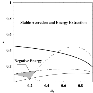
(a)

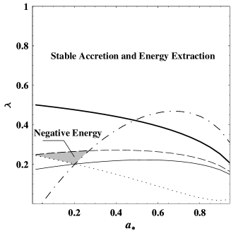
(b)

Figure 7: The contours of $P_{PL}=0$ (dashed line), $dS_{H}/dt=0$ (dotted line), $\dot{M}_{D}=0$ (solid line), $F_{Acc}=1$ (dot-dashed line) and $F_{Energy}=0$ (thick solid line) in $a_{*}-\lambda$ parameter space with $0<a_{*}<0.9428$ and $0<\lambda<1$ for (a) $\alpha_{m}=0.039$ and (b) $\alpha_{m}=0.030$.

In Figure 7 the shaded region indicated ”Negative Energy” is bounded by four contours, i.e. $P_{PL}\leq 0$, $dS_{H}/dt\geq 0$, $\dot{M}_{D}\geq 0$ and $F_{Acc}\geq 1$ in dashed, dotted, solid dot-dashed lines, respectively. However, the negative energy is excluded by the contour of $F_{Energy}\geq 0$ in thick solid line, above which the stable energy extraction from the plunging particles is required. The region above the thick solid line and the dot-dashed line is indicated ”Stable Accretion and Energy Extraction”, in which energy extraction via MCPD can work in a stable way.

Thus we conclude, although the negative energy can be delivered to the BH via MCPD with the validity of the second law of the BH thermodynamics, it cannot be realized in a stable way in our model.

5 EFFECTS OF MCPD AND MCHD ON EFFICIENCY OF ENERGY RELEASE

Although MCHD and MCPD are related to the magnetic field configuration supported by a toroidal current flowing on the equatorial plane of the Kerr BH, these two mechanisms are different in several aspects.

(1) Energy and angular momentum are extracted and transferred from the Kerr BH to the disc by virtue of MCHD, while those are extracted and transferred from the plunging particles to the inner disc by virtue of MCPD.

(2) MCHD can work in a suspended accretion state as suggested by van Putten & Ostriker (2001), while MCPD cannot operate without continuous replenishment of accreting particles.

Therefore a stable accretion and energy extraction are indispensable in the model containing the coexistence of MCHD and MCPD. Based on the BH evolution equation (53), we can easily obtain the efficiencies of releasing energy as follows.

$$\eta=1-{\left({{dM}\mathord{\left/{\vphantom{{dM}{dt}}}\right.\kern-1.2pt}{dt}}\right)}\mathord{\left/{\vphantom{{\left({{dM}\mathord{\left/{\vphantom{{dM}{dt}}}\right.\kern-1.2pt}{dt}}\right)}{\dot{M}_{D}}}}\right.\kern-1.2pt}{\dot{M}_{D}}=\eta_{{}_{D}A}+\eta_{MC}^{HD}+\eta_{MC}^{PD},$$ (69)

where $\eta_{{}_{D}A}$, $\eta_{MC}^{HD}$ and $\eta_{MC}^{PD}$ are respectively the efficiencies due to disc accretion, MCHD and MCPD, converting the rest energy of the accreting particles into the radiation energy. These efficiencies are expressed as

$$\left\{{\begin{array}[]{l}\eta_{{}_{D}A}=1-E_{ms},\\ \eta_{MC}^{HD}={P_{MC}^{HD}}\mathord{\left/{\vphantom{{P_{MC}^{HD}}{\dot{M}_{D}}}}\right.\kern-1.2pt}{\dot{M}_{D}},\\ \eta_{MC}^{PD}={P_{MC}^{PD}}\mathord{\left/{\vphantom{{P_{MC}^{PD}}{\dot{M}_{D}}}}\right.\kern-1.2pt}{\dot{M}_{D}}.\end{array}}\right.$$ (70)

Incorporating equation (70) with the concerning expressions for $E_{ms}$, $\dot{M}_{D}$, $P_{MC}^{HD}$ and $P_{MC}^{PD}$, we have the curves of $\eta_{{}_{D}A}$, $\eta_{MC}^{PD}$ and $\eta_{MC}^{HD}$ versus $a_{*}$ for the different values of $\alpha_{m}$ and $\lambda$ as shown in Figure 8.

(a)

(b)

Figure 8: The curves of $\eta_{{}_{D}A}$, $\eta_{MC}^{PD}$ and $\eta_{MC}^{HD}$ versus $a_{*}$ respectively in solid, dashed and dotted lines for (a) $\alpha_{m}=0.039$, $\lambda=0.55$ and (b) $\alpha_{m}=0.03$, $\lambda=0.6$.

The efficiency $\eta_{MC}^{PD}$ is greater (less) than $\eta_{MC}^{HD}$ for the lower (higher) BH spin, while it is generally less than $\eta_{{}_{D}A}$ as shown in Figure 8. In order to compare the efficiencies $\eta_{MC}^{PD}$ and $\eta_{{}_{D}A}$ in an accurate way we have the contours of ${\eta_{MC}^{PD}}\mathord{\left/{\vphantom{{\eta_{MC}^{PD}}{\eta_{{}_{D}A}}}}\right.\kern-1.2pt}{\eta_{{}_{D}A}}=1$, $F_{Acc}=1$ and $F_{Energy}=0$ in $a_{*}-\lambda$ parameter space as shown in Figure 9.

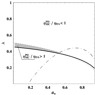
(a)

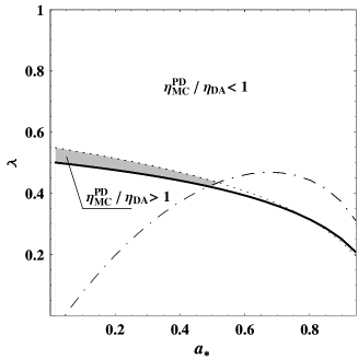
(b)

Figure 9: Contours in $a_{*}-\lambda$ parameter space of $\eta_{MC}^{PD}/\eta_{{}_{D}A}=1$, $F_{Energy}=0$ and $F_{Acc}=1$ in dotted, solid and dot-dashed lines, respectively. The parameter $\alpha_{m}$=0.039 and 0.03 are given in Figures 10a and 10b, respectively.

Inspecting Figure 9, we find that efficiency $\eta_{MC}^{PD}$ is generally less than $\eta_{{}_{D}A}$ in a wide value range of $a_{*}$ and $\lambda$ for the given values of $\alpha_{m}$, and the possibility of $\eta_{MC}^{PD}>\eta_{{}_{D}A}$ is confined in a very narrow shaded region indicated by “${\eta_{MC}^{PD}}\mathord{\left/{\vphantom{{\eta_{MC}^{PD}}{\eta_{{}_{D}A}}}}\right.\kern-1.2pt}{\eta_{{}_{D}A}}>1$” in Figure 9.

6 DISCUSSION

In this toy model the magnetic field configuration is generated by a single electric current flowing at ISCO of a thin disc, and we regard this as a starting point for dealing with the magnetic field configuration generated by the electric current distributed in more realistic way around a BH. We concentrate the discussion on the magnetic extraction of energy and angular momentum from the plunging particles, and we describe our model phenomenally by using two parameters instead of resolving the extremely complicated MHD equations within ISCO. The parameter $\lambda$ is used to describe the angular velocity of the plunging particles, and the parameter $\alpha_{m}$ is invoked to adjust the accretion rate affected by MCPD. It is noted that the parameters $a_{*}$, $\lambda$ and $\alpha_{m}$ are crucial for a stable MCPD process, although the MCPD power and torque are independent of the parameter $\alpha_{m}$ according to equations (49)–(51).

The key point in this model is how to constrain these parameters based on some reasonable considerations. In this model four requirements are given: (i) a positive accretion rate, (ii) an increasing BH entropy, (iii) a stationary accretion and (iv) a stable energy extraction for the plunging particles. Required by these constraints the following results are obtained in our model.

(1) MCPD could be more important than MCHD in transferring energy and angular momentum to the disc. As shown in Figures 4–6, the power and torque in MCPD are stronger than those in MCHD for low BH spins.

(2) Although negative energy can be delivered to the BH by the plunging particles with the increasing BH entropy it cannot be realized via MCPD in a stable way as shown in Figure 7.

The efficiency of releasing energy due to MCPD could be greater than that due to MCHD for low BH spins, while it is generally less than the efficiency of disc accretion for a wide range of $a_{*}$ and $\lambda$ as shown in Figure 9.

It is assumed in $\S$ 2.2 that the toroidal current located at $r_{ms}$ has a very small circular section of radius ${r}^{\prime}_{\varepsilon}=\varepsilon r_{ms}$, and $\varepsilon=10^{-4}$ is taken in calculations. The parameter $\varepsilon$ is introduced to avoid an infinite magnetic field as $r$close to the toroidal current. The magnetic field outside ${r}^{\prime}_{\varepsilon}=\varepsilon r_{ms}$ are not affected by the value of $\varepsilon$, while the contribution of the magnetic field to the MCPD effects can be neglected if $\varepsilon$ is small enough. Thus the influences of $\varepsilon$ on the MCPD effects are very little. For example, required by ${P_{MC}^{PD}}\mathord{\left/{\vphantom{{P_{MC}^{PD}}{P_{MC}^{HD}}}}\right.\kern-1.2pt}{P_{MC}^{HD}}=1$with $a_{\ast}$=0.294, we have $\lambda$=0.6187569089, 0.6187569092 and 0.6187569342 for $\varepsilon$= 10^-5, 10^-4 and 10^-3, respectively. The variation of $\lambda$ arising from that of $\varepsilon$ is ${\Delta\lambda}\mathord{\left/{\vphantom{{\Delta\lambda}{\Delta\varepsilon}}}\right.\kern-1.2pt}{\Delta\varepsilon}<3\times 10^{-5}$.

Another issue related to our model lies in prescription (44), in which the surface resistivity of the plunging region is assumed to be $R_{{PL}}={R}_{H}=4\pi$. The resistivity ${R}_{H}$ is defined such that the electric field at the BH horizon is equal in magnitude to the magnetic field. We can show that the prescription (44) does not lead to the result that the electric field at the surface of the plunging region is greater than the magnetic field there.

The toroidal component of the magnetic field at the surface of the disc is expressed by equation (25). Similarly, we can derive the expressions for the toroidal magnetic field at the surface of the plunging region as follows,

$$B_{PL}^{T}={2I_{MC}^{PD}}\mathord{\left/{\vphantom{{2I_{MC}^{PD}}{\left({\varpi_{PL}\alpha}\right)_{\theta=\pi\mathord{\left/{\vphantom{\pi 2}}\right.\kern-1.2pt}2}}}}\right.\kern-1.2pt}{\left({\varpi_{PL}\alpha}\right)_{\theta=\pi\mathord{\left/{\vphantom{\pi 2}}\right.\kern-1.2pt}2}}.$$ (71)

The toroidal electric field is zero in a stationary axisymmetric magnetosphere (MT82), while the poloidal electric field at the surface of the plunging region is related to $I_{MC}^{PD}$ by Ohm’s law, i.e.,

$$\alpha E_{PL}=R_{{PL}}{I_{MC}^{PD}}\mathord{\left/{\vphantom{{I_{MC}^{PD}}{2\pi\varpi_{PL}}}}\right.\kern-1.2pt}{2\pi\varpi_{PL}},$$ (72)

where $\alpha E_{PL}$ is the electric field converted to a ‘per unit globe time’ basis (MT82). Incorporating equations (25) and (72) we have

$${E_{PL}}\mathord{\left/{\vphantom{{E_{PL}}{B_{PL}^{T}}}}\right.\kern-1.2pt}{B_{PL}^{T}}={R_{{PL}}}\mathord{\left/{\vphantom{{R_{{PL}}}{4\pi}}}\right.\kern-1.2pt}{4\pi}.$$ (73)

Thus the prescription (44) leads to $E_{PL}=B_{PL}^{T}$ and $E_{PL}<B_{PL}=\sqrt{\left({B_{PL}^{T}}\right)^{2}+\left({B_{PL}^{P}}\right)^{2}}$.

In this paper we do not fit the very steep emissivity observed in some BH systems, such as galaxy MCG-6-30-15. In fact, a very steep emissivity can be also produced by virtue of MCPD, since the energy and angular momentum transferred from the plunging region are very concentrated in the inner disc. We shall work out a more realistic model to relate MCPD to the observations in our future work.

References

- [1] Bardeen, J. M., Press, W. H. & Teukolsky, S. A., 1972, ApJ, 178, 347
- [2] Bateman, G., MHD Instabilities, 1978, (Cambridge: The MIT Press)
- [3] Blandford, R. D., & Znajek R. L., 1977, MNRAS, 179, 433
- [4] Blandford, R. D., 1999 in Astrophysical Discs: An EC Summer School, Astronomical Society of the Pacific Conference Series, ed. Sellwood J A & Goodman J 160, 265
- [5] Blandford, R. D., 2002, Lighthouses of the Universe: The Most Luminous Celestial Objects and Their Use for Cosmology Proceedings of the MPA/ESO/, p. 381.
- [6] Kadomtsev, B. B. 1966, Rev. Plasma Phys., 2, 153
- [7] Li, L. -X. 2000a, ApJ, 533, L115
- [8] —. 2000b, ApJ, 540, L17 (L00)
- [9] —. 2002a, A&A, 392, 469
- [10] —. 2002b, Phys. Rev. D. 65 084047 (L02)
- [11] Linet, B., 1979, J. Phys. A 12, 839
- [12] Macdonald, D., & Thorne, K. S., 1982, MNRAS, 198, 345 (MT82)
- [13] Moderski, R., Sikora, M., & Lasota, J.P., 1997, in “Relativistic Jets in AGNs” eds.M. Ostrowski, M. Sikora, G. Madejski & M. Belgelman, Krakow, p.110
- [14] Novikov, I. D., & Thorne, K. S., 1973, in Black Holes, ed. Dewitt C, (Gordon and Breach, New York) p.345
- [15] Page D. N., & Thorne K. S., 1974, ApJ, 191, 499
- [16] Shapiro, S. L., & Teukolsky, S. A., (1983). Black Holes, White Dwarfs and Neutron Stars, ( John Wiley and Sons, Inc. New York). P.357
- [17] Thorne K. S., Price R. H., & Macdonald D. A., 1986, Black Holes: The Membrane Paradigm, Yale Univ. Press, New Haven
- [18] Uzdensky, D. A., 2005, ApJ, 620, 889
- [19] van Putten, M. H. P. M., & Ostriker, E. C., 2001, ApJ, 552, L31;
- [20] Wang, D.-X., Xiao, K., & Lei, W.-H., 2002, MNRAS, 335, 655 (W02)
- [21] Wang, D.-X., Ma, R.-Y., Lei W.-H., & Yao, G.-Z. 2003, ApJ, 595, 109 (W03)
- [22] —. 2004, ApJ, 601, 1031
- [23] Wilms, J, et al. 2001, MNRAS, 328, L27
- [24] Znajek, R. L., 1978, MNRAS, 182, 639