Cosmological evolution with a logarithmic correction in the dark energy entropy

Abstract

In a thermodynamical model of cosmological FLRW event horizons for the dark energy (DE), we consider a logarithmic corrective term in the entropy to which corresponds a new term in the DE density. This model of $\Lambda(t)$ in an interacting two-component cosmology with cold dark matter (DM) as second component leads to a system of coupled equations, yielding, after numerical resolution, the evolutions of $\Lambda(t)$, the Hubble $H(t)$, vacuum density $\Omega_{\Lambda}(t)$, deceleration $q(t)$ and statefinder $R(t)$ and $S(t)$ parameters. Its results, compatible with an initial inflation and the current observations of the so-called “concordance model”, predict a graceful exit of early inflation and the present acceleration and solve in the same time the age and coincidence problems. Moreover they account for the low-$l$ CMBR power spectrum suppression.

keywords : Dark energy theory, SnIa constraints, CMBR (low multipoles) theory.

1 Introduction

The observations of SNe of type Ia [1][2], showing that the universe has probably recently entered on a phase of acceleration, raised up a renewal of interest in the cosmological constant (CC) problem [3] [4].

Since then an increasing number of observational evidences for such an acceleration has been settled. This acceleration together with other cosmological indicators such as the flatness ($k=0$) from the CMB anisotropies observed by Boomerang, Proxima and WMAP [5], the present values $H_{0}$ by the HST key project [6], $\Omega_{b0}$ and $\Omega_{m0}$ by observations of the light elements, SBBN and cluster baryon fraction from X-ray emission [7]), led to the so-called “concordance model” [8] based on the $\Lambda$CDM model. This model is the simplest improvement of the old standard cosmological model (including inflation). More precisely, the simplest theoretical candidate explaining this accelerated expansion is a cosmological constant $\Lambda$, or some component, called dark energy (DE): any term in the energy-momentum tensor which can produce the same negative pressure, such as a scalar field [9], called quintessence [10], or a bulk viscosity [11].

However, the re-introduction of the CC $\Lambda$ leads to new intriguing puzzles. Particularly, we have to face the old CC problem: the discrepancy between the predictions of the effective Quantum fields theory concerning the large vacuum energy density and the tiny upper limits observed in astrophysics for the CC. Besides, it gives rise to a new issue, the so-called “coincidence problem”, where one has to explain why the CC starts recently to dominate the matter. Assuming $\Lambda=constant$, it can only be solved by an unsatisfying fine-tuning. Finally, the introduction of $\Lambda$ needs also to be conciliated with the inflation in the early universe.

In these conditions, we have to improve the $\Lambda CDM$ model in order to solve these puzzling issues.

Therefore, we propose a $\Lambda(t)CDM$ model, namely the simplest modification of the $\Lambda CDM$ model which allows the best account of the theoretical expectations and the observed data. Some “ansatze” were already proposed to solve the CC problem before the discovery of the present universe acceleration (for a review, see [12]). By contrast, the present model, namely the event horizon Thermodynamics (ehT) model, is derived from a thermodynamical approach and not based on an ad hoc hypothesis for the law $\Lambda(t)$. Such a phenomenological model is an indispensable preliminary to outline the main laws that any further treatment at the statistical or/and quantum level will have to reproduce, as for example the Stefan’s law has guided the Planck law’s advent for the black body radiation. We thus proposed a model with a variable vacuum energy density [13][14], based on the generalization of the Thermodynamics of the black hole event horizons (BH e.h.)[15] to the Friedmann-Lemaître-Robertson-Walker event horizons (FLRW e.h.)[16]. This model allows to reconstitute the entire evolution from the early inflation to late acceleration (for another approach, see also [17]).

In this article, we extend this phenomenological model by introducing a logarithmic correction in the $\Lambda$-entropy. Such a corrective term in the entropy was recently computed for the entropy of any thermodynamical system and applied to Black Hole by S.Das et al. [18]. This correction due to statistical fluctuations around an equilibrium state has an universal character. As the cosmological FLRW e.h. presents notable thermodynamical analogies with the BH e.h. (albeit some differences [19]), we examine the effects of the introduction of this new term in the $\Lambda(t)CDM$ model. It appears that the derived expression for $\Lambda(r)$, with $r$ the radius of the event horizon (e.h.), can then be naturally interpreted as a renormalisation relation and allows to describe the main observed features of the evolution of the universe. In this scheme, the obtained universe is initially submitted to a local phase of de Sitter inflation ($\Omega_{\Lambda}(0)=1$). The vacuum density parameter begins to decrease and there is a graceful exit of inflation. The parameter $\Omega_{\Lambda}$ passes through a small minimum, then grows again, which allows to solve the “coincidence problem”. It tends asymptotically to a de Sitter universe. At any instant $t$, $H(t)$ and $\Lambda(t)$ are decreasing functions.

The paper is organized as follows. In Section 2, we set the basis of the general relativistic framework in which our model for $\Lambda(t)$ will be developed. In Section 3, we present the ehT model for the vacuum (or DE) energy density. Then in Section 4, we examine the influence of the entropy’s correction term in the vacuum energy density and its relevance in the renormalisation approach. In Section 5, we deduce the equations of evolution for $H(t)$ and $r(t)$, and present in section 6, their numerical resolution, in particular, the graphic of $\Omega_{\Lambda}(t)$. Section 7 is devoted to a brief conclusive summary.

2
An interacting two-component model

Let us briefly recall the minimal assumptions underlying our model.

In order to set our notations, let us first write the Einstein equations:

$$R_{\alpha\beta}-\frac{R}{2}g_{\alpha\beta}+\Lambda_{0}g_{\alpha\beta}=\chi T_{\alpha\beta}\text{.}$$ (1)

with $\chi=\frac{8\pi G}{c^{4}}$ and $\Lambda_{0}$ a positive constant (the GR bare cosmological constant). Only for this choice of coefficients in Eq. (1), the Bianchi identity $\nabla_{\beta}T^{\alpha\beta}=0$ is satisfied [20][21].

Assuming a perfect fluid of energy density $\rho_{T}$ and pressure $P_{T}$, the energy-momentum tensor is given by $T_{\alpha\beta}=\rho_{T}u_{\alpha}u_{\beta}-P_{T}\Delta_{\alpha\beta}$ with $\Delta_{\alpha\beta}:=g_{\alpha\beta}-u_{\alpha}u_{\beta}$, and the index ”$T$” means ”Total”.

Following [13] and [14], the perfect fluid is supposed to admit two components: $\rho_{T}=\rho_{1}+\rho_{2}$ and $P_{T}=P_{1}+P_{2}$.

The first one corresponds to vacuum, i.e., it obeys the “pseudo-barotropic” equation of state : $P_{1}=\omega\rho_{1}$ with $\omega=-1$.

The second component obeys a barotropic equation of state given by $P_{2}=(\gamma-1)\rho_{2}$. In section 6, we consider dust ($\gamma=1$).

In accordance with the WMAP observational results of the CMB’s anisotropies [5], the metrics is taken to be the spatially flat ($k=0$) FLRW metrics. With these assumptions, Equation (1) reduces to

$$R_{\alpha\beta}-\frac{R}{2}g_{\alpha\beta}=\Lambda g_{\alpha\beta}+\chi T_{2\alpha\beta}$$ (2)

with $T_{2\alpha\beta}:=\rho_{2}u_{\alpha\beta}-P_{2}\Delta_{\alpha\beta}$ and

$$\Lambda:=\Lambda_{vac}-\Lambda_{0}.$$ (3)

As $\Lambda_{vac}:=\chi\rho_{1}$ with $\rho_{1}$ variable, $\Lambda$ varies. In the following, we refer to $\Lambda$ as the “ variable cosmological constant”. It can be considered as an “effective” CC. The corresponding dark energy (DE)-component has the energy density : $\rho_{\Lambda}=\frac{\Lambda}{\chi}$.

We do not make any further assumption on a separated energy conservation for each component. In the old standard cosmological model, this assumption is made only for each era of “domination” of one component (e.g. “era dominated by the radiation”, “era dominated by the matter”, today “era dominated by the DE”, or in the very early universe “era dominated by the inflation (or the inflaton)”). If such an assumption can seem reasonable for these domination eras (and so appears more as an approximation), it is not the case for the transient periods, as for instance the very recent epoch of transition from dark matter (DM) to DE domination.

Anyway, the complete energy conservation due to the Bianchi identity is more general than the separated conservations, which necessitate some supplementary assumption. For example, in the $\Lambda(t)$ and quintessence models, a separated conservation law for each component implies a “variable” equation of state. By contrast, the present model assumes the equations of state in a thermodynamical sense, i.e. given once for all, with an interaction between the two components. This kind of approach with components interaction has already been considered (see e.g. [22][23]).

Let us sketch the rough scenario of the universe evolution. Initially, setting $\rho_{1}=\rho_{Max}$ and $\rho_{2}=\rho_{2\min}\simeq 0$, the universe undergoes a de Sitter inflation, with $\Lambda_{M}=\Lambda_{vacM}-\Lambda_{0}>0$. Then $\rho_{1}$ decreases or equivalently, $\Lambda$ decreases with the universe expansion. In the same time, $\rho_{2}$ is increasing. Finally, $\rho_{1}$ tends to $\Lambda_{0}$ or equivalently $\Lambda$ tends to $\Lambda_{\min}\simeq 0$ ,which is again a de Sitter evolution. Today, we observe a very small value for $\Lambda=\chi\rho_{1}-\Lambda_{0}$ with a very large vacuum energy density $\rho_{1}$ given by quantum field theory (today $\rho_{1}$ is of the order of $\Lambda_{0}$). For a reasonable (Planck) largest cut-off, we obtain $\frac{\Lambda}{\chi\rho_{1}}=1-\frac{\Lambda_{0}}{\chi\rho_{1}}\sim 10^{-120}$. Assuming a variable cosmological “constant” solution (as considered here), this scheme appears as an hardly intelligible fine-tuning. It is the so-called “old problem” of the cosmological constant (CC). Besides, the recent domination of the vacuum energy by dust constitutes the “new puzzle” of the CC (or “coincidence problem”). At the beginning, $\rho_{2}$ represents the energy density of the radiation and the ultrarelativistic matter. For sake of simplicity, we shall only consider in the following (section 6) the non relativistic matter ($\gamma=1$).

We propose a phenomenological model of this DE or, equivalently, this variable cosmological “constant” (or this vacuum energy density) able to produce the main properties of this scenario. More particularly, the two problems of the CC are solved in the framework of our model where $\Lambda$ runs from a large initial value $\Lambda_{M}$ (a huge inflation in the very early universe) to a weak final constant $\Lambda_{m}$ which yet starts again to dominate, leading to “the coincidence problem”. In the two cases, the same DE, with a density $\Lambda$ is used to explain the universe acceleration. This DE is negligible or dominates, depending on the considered period, and its density decreases all along the universe expansion.

3 Thermodynamical model of the cosmological FLRW e.h.

The variable DE density $\Lambda=\chi\rho_{\Lambda}$ is the first component of the two perfect fluids constitutive of the universe. In the de Sitter space-time, this cosmological “constant”, or vacuum energy density, obeys the equations of state [15][24]:

$$\Lambda+\chi P_{\Lambda}=0$$ (4)

$$\Lambda=\frac{3k^{2}}{c^{2}\text{h{\hskip-1.99997pt}\hbox to0.0pt{\hss\rule[4.73611pt]{3.24997pt}{0.43057pt}}{\hskip 1.99997pt}}^{2}}T_{\Lambda}^{2}$$ (5)

where $P_{\Lambda}$ and $T_{\Lambda}$ represent its (negative) pressure and its temperature respectively, h   is the Planck constant, $c$ the light velocity and $k$ the Botlzmann constant. Each thermodynamical variable is linked to the proper radius $r$ of the event horizon at a given instant by the relations

$$T_{\Lambda}=\frac{\text{h{\hskip-1.99997pt}\hbox to0.0pt{\hss\rule[4.73611pt]{3.24997pt}{0.43057pt}}{\hskip 1.99997pt}}c}{kr}\text{ ,}$$ (6)

$$\Lambda=\frac{3}{r^{2}}\text{ .}$$ (7)

We can also introduce the horizons number density $n_{\Lambda}$ defined as usual in Thermodynamics by the inverse of the specific volume of the horizon [13]

$$n_{\Lambda}=\frac{3}{4\pi r^{3}}\text{ .}$$ (8)

Introducing the expression (6) of the temperature in the preceding relation, we obtain a third equation of state:

$$n_{\Lambda}=\frac{3}{4\pi}(\frac{k}{\text{h{\hskip-1.99997pt}\hbox to0.0pt{\hss\rule[4.73611pt]{3.24997pt}{0.43057pt}}{\hskip 1.99997pt}}c})^{3}T_{\Lambda}^{3}=\frac{\Lambda^{\frac{3}{2}}}{4\pi\sqrt{3}}\text{.}$$ (9)

Equation (9) together with Eq. (4) and (5) define a local equilibrium state for the DE component in the de Sitter spacetime. Let us now consider the same DE component in the spatially flat FLRW space-time. The three thermodynamical equations of state (4), (5) and (9) have to remain valid in FLRW spacetime because the thermodynamical equations of state of any actual component (e.g. $P=\frac{\rho}{3}$, or the Stefan law $\rho=\sigma T^{4}$, for the equilibrium radiation) are always supposed to be independent of the chosen spacetime. Besides, the definition (8) of $n_{\Lambda}$ remains also valid in the (spatially flat) FLRW spacetime. Consequently, from (8) and (9), we find that this DE component is associated to the FLRW e.h. via the relation (7). Using (7), (8) and (9), we obtain the expression (6) for $T_{\Lambda}$ and (5) for $\Lambda$ in the FLRW spacetime too.

Relation (7) has also been independently derived from holographic principle [25]. Albeit the choice of $r$ is not necessarily a priori given in the holographic approach (e.g. the Hubble horizon $H^{-1}$ can be chosen instead [26][27], or the particle horizon $r_{p}$ as well [28]), it is the unique choice in this framework that leads to an admissible equation of state [29] and which is strongly supported by the SnIa observational results [30][14].

Differentiating the definition of $r$ with respect to the time (e.g. see eqs.(3.4) and (3.6) in [13] or (9) and (10) in [14])) yields the relation

$$H-\frac{\overset{\cdot}{r}}{r}=\frac{c}{r}$$ (10)

where $H$ is the Hubble parameter and the dot means the time derivative.

In order to set a complete local thermodynamics, we need to determine the entropy density $ns_{\Lambda}$ where $s_{\Lambda}$ is the specific entropy. To reach this goal, we use the Gibbs equation which at the specific level is given by:

$$T_{\Lambda}ds_{\Lambda}=d\varepsilon_{\Lambda}+P_{\Lambda}dv_{\Lambda}$$ (11)

where $\varepsilon_{\Lambda}\equiv\displaystyle\frac{\Lambda}{n_{\Lambda}\chi}$ is the specific energy, $v_{\Lambda}\equiv\frac{1}{n_{\Lambda}}$ the specific volume. With Eq. (4), we deduce

$$\chi n_{\Lambda}T_{\Lambda}d{s_{\Lambda}}=d\Lambda\text{.}$$ (12)

4 Fluctuations and renormalization

In a recent article, a logarithmic corrective term in the expression of the entropy of any thermodynamical system was derived by S.Das et al. [18]. This correction due to small thermal fluctuations around an equilibrium reads for BH entropy:

$$s=\pi r^{2}-\alpha^{\prime}\ln\pi r^{2}$$ (13)

where $\alpha^{\prime}$ is a constant. Introducing the same correction in the cosmological eh model, the expression of the specific entropy becomes

$$s_{\Lambda}=-4(\frac{k}{L_{P}^{2}})(\pi r^{2}+2\pi\alpha\ln\pi r^{2})+C,$$ (14)

where $L_{P}$ is the Planck length (defined by $L_{P}^{2}:=\chi$h  $c=4l_{P}^{2}$, with $l_{P}^{2}:=\frac{Gh}{c^{3}}$ in the I.S. units), $\alpha$ is a constant of dimension $[r^{2}]$ and $C$ an arbitrary constant. As usual, the sign of the entropy is negative for the cosmological horizon (e.g. [16] [13]). As noticed by S.Das et al. [18] and Major and Setter [31], when there is not conservation of the number of particles in an open sytem, the sign “-” before the $\alpha$-term has to be replaced by a sign “+”. This is precisely the case here for our $\Lambda$-component, which is not separately conserved.

Let us split the constant $C$ into

$$C=4\pi\frac{k}{L_{P}^{2}}(2\alpha\ln\pi r_{2}^{2}+r_{3}^{2}\text{ ),}$$ (15)

where $r_{2}$ is associated to the corrective term and $r_{3}$ to the expression of $s_{\Lambda}$ without correction. The expression of $s_{\Lambda}$ becomes

$$s_{\Lambda}=8\pi\frac{k}{L_{P}^{2}}\alpha(\frac{r_{3}^{2}-r^{2}}{2r_{1}^{2}}-\ln\frac{r^{2}}{r_{2}^{2}})\text{.}$$ (16)

The constant factor $\alpha:=r_{1}^{2}$ has the dimensions of a surface. Let us remark the omission of the Bekenstein factor $\frac{k}{l_{P}^{2}}$ in most papers by choice of the Planck units ($h=c=k=G=1$). The expressions of $r_{2}$ and $r_{3}$ are constrained by setting

$$\left|\frac{r_{3}^{2}-r^{2}}{2r_{1}^{2}}\right|\gg\left|\ln\frac{r^{2}}{r_{2}^{2}}\right|\text{ , }\forall r\geq r(0)$$ (17)

where $r(0)$ is the initial event horizon (see Section $6$). The simplest choice for $r_{2}$ and $r_{3}$ is given by $r_{2}=r_{3}=r_{M}$ , where $r_{M}$ is the maximum radius (possibly infinite). Hence, $s_{\Lambda}$ is always positive with $s_{\Lambda}=0$ when $r=r_{M}$. For $r=r_{M}-\epsilon$ with $\epsilon\ll r_{M}$, we deduce $r_{3}^{2}-r^{2}\simeq 2\epsilon r_{M}$ and $2r_{1}^{2}\ln(\frac{r_{M}^{2}(1-2\frac{\epsilon}{r_{M}})}{r_{M}^{2}})\simeq-2r_{1}^{2}\frac{2\epsilon}{r_{M}}$. A corrective term is only obtained if $r_{1}\ll r_{M}$ as will be verified in Section 6. Finally, for $r=r_{m}$, we have $(r_{M}^{2}-r_{m}^{2})-2r_{1}^{2}\ln((\frac{r_{m}}{r_{M}})^{2})\simeq r_{M}^{2}+4r_{1}^{2}\ln(\frac{r_{M}}{r_{m}})$. For $r_{1}\ll r_{M}$ , the $\ln$-term is a corrective term and tends to $s\rightarrow s_{M}=\frac{8\pi k}{L_{P}^{2}}r_{M}^{2}$. It follows that $r_{1}$ has not necessarily to be very small with respect to $r$ but only with respect to $r_{M}$.

Let us examine the effects of such a new term in $s_{\Lambda}$ (14) on the expression of $\Lambda$ .

Differentiating Eq.(14) for $s_{\Lambda}$ with respect to $r$ and introducing this expression into Equation (12) with (6) and (8), we obtain a differential equation for $\Lambda$ and $r$, which yields after integration

$$\Lambda=\frac{3}{r^{2}}(1+(\frac{r_{1}}{r})^{2})\text{ , }r_{1}^{2}:=\alpha\geq 0\text{,}$$ (18)

where the boundary conditions are set such that $\Lambda$ tends to $0$ when $r\rightarrow\infty$. This relation is an extension of the expression (7) of $\Lambda$ when thermodynamical fluctuations are taken into account.

It is worth noting that this relation is strongly akin to a renormalization relation (e.g. see first Eq.(3.3) in [32], or Eq. (33) in [33], see also [34]). In the same way, Padmanabhan ([35], Eq.(19)) and Myung ([36], Eq. (14)) write a renormalized vacuum energy density by stressing a hierarchical structure of the form:

$$\rho_{vac}=\frac{3\text{h{\hskip-1.99997pt}\hbox to0.0pt{\hss\rule[4.73611pt]{3.24997pt}{0.43057pt}}{\hskip 1.99997pt}}c}{L_{1}^{2}L_{P}^{2}}[1+(\frac{L_{1}}{L})^{2}+(\frac{L_{1}}{L})^{4}+...]\text{,}$$ (19)

where the first term is interpreted as the energy density necessitating to be renormalized, the second term as the vacuum fluctuations and the third one as the de Sitter thermal energy density (the dimensional constants and the factor $3$ were restored for convenience). Padmanabhan and Myung have introduced this form in the case $L_{1}=L_{P}$, here we use an intermediate scale $L_{1}$ greater than $L_{P}$. A value of $L_{1}$ accurate to observational results will be determined in Section 6. Setting $\Lambda_{1}:=\frac{3}{L_{1}^{2}}$, and multiplying the relation (19) by $\chi$, we obtain:

$$\Lambda_{vac}-\Lambda_{1}=\frac{3}{L^{2}}[1+(\frac{L_{1}}{L})^{2}+...]\text{.}$$ (20)

Assuming $\Lambda_{1}$ to be the bare CC $\Lambda_{0}$ of the G.R. (eqs. (1) and (3)), this expression is of the same form as the expression (18) derived in our model. Let us discuss an intriguing point. The second term in the r.h.s. of (18) has by construction to be interpreted as a term of fluctuations, whereas it is the first one in the r.h.s. of (20) which is interpreted as fluctuations by Padmanabhan and Myung. Let us consider the solution to this apparent discrepancy. Relation (18) is derived from considerations concerning fluctuations by use of a Taylor expansion. It can be considered in the framework of renormalization as the truncature of a convergent series up to its first terms (see [33] after their Eq. (35)). In particular, Eq. (18) is valid for the two following limits:

For $r\gg r_{1}$, Eq (18) represents the first terms of a Taylor expansion and $\Lambda$ tends to (7) which itself tends to its minimal constant limit $\Lambda_{m}=\frac{3}{r_{M}^{2}}$ when $r$ tends to its maximum limit $r_{M}$ (IR cutoff). For these large values of $r$, we are concerned with the inflation undergone today by the universe. Therefore the fluctuations we considered in (14) and (18) are these recent fluctuations. In this limit, the model (7) was studied in [14].

For $r\ll r_{1}$, Eq (18) can be rewritten as a Taylor expansion for little values of $r$

$$\Lambda=\frac{3r_{1}^{2}}{r^{4}}(1+(\frac{r}{r_{1}})^{2})\text{,}$$ (21)

and $\Lambda$ tends towards another de Sitter state when $r$ reaches its minimum limit $r_{m}$ (UV cutoff). For these values of $r$, what is concerned is the maximum value of $\Lambda$, during the inflation formerly undergone by the very early universe: $\Lambda_{M}=\frac{3r_{1}^{2}}{r_{m}^{4}}$. Padmanabhan and Myung consider these early fluctuations in (19).

Considered as a renormalisation relation, Eq. (18) is also valid for any intermediate value of $r$ and especially when $r\equiv r_{1}$. Assuming the given expression (18) for $\Lambda$, we derive now the evolution of the universe.

5 Evolution equations for H and r

In a spatially flat FLRW cosmology ($k=0$, metrics signature + - - -), the field equations (2) for a two-component perfect fluid with the variable CC as first component are given by

$$(\Lambda+\chi\rho)c^{2}=3H^{2}$$ (22)

$$\overset{\cdot}{H}\text{ }=-\frac{\gamma}{2}\chi c^{2}\rho\text{ .}$$ (23)

From now on, the index 2 for the second component of the fluid is understood. Equations (22) and (23) lead to

$$\overset{\cdot}{H}\text{ }=-\frac{\gamma}{2}(3H^{2}-\Lambda c^{2})\text{.}$$ (24)

By defining

$$Y:=\frac{1}{r^{2}}\text{ ,}$$ (25)

(24) and (10) become

$$2\overset{\cdot}{H}+3\gamma H^{2}-3\gamma c^{2}Y(1+\alpha Y)=0$$ (26)

$$\overset{\cdot}{Y}+2HY-2cY^{\frac{3}{2}}=0\text{ ,}$$ (27)

where the expression (18) of $\Lambda$ has been introduced. Eqs (26) and (27) constitute a system of two coupled first order differential equations satisfied by {$Y(t),H(t)$}. We introduce the dimensionless variables

$$y:=\frac{Y}{Y_{1}}\text{ , }h:=\frac{H}{H_{1}}\text{ ,}$$ (28)

where $Y_{1}$ and $H_{1}$ are two, a priori independent, arbitrary constant scales for $Y$ and $H$ respectively. We also define the dimensionless time $\tau$

$$\tau:=(H_{1}t)^{n}\text{ , (}n>0\text{).}$$ (29)

Hence, (26) and (27) become

$$2n\tau^{\frac{n-1}{n}}h^{\prime}+3\gamma h^{2}-3\gamma X_{1}y(1+\alpha_{1}y)=0$$ (30)

$$n\tau^{\frac{n-1}{n}}y^{\prime}+2hy-2\sqrt{X_{1}}y^{\frac{3}{2}}=0\text{ ,}$$ (31)

with

$$X_{1}:=\frac{Y_{1}c^{2}}{H_{1}^{2}}$$ (32)

the dimensionless ratio of the scales $Y_{1}$ and $H_{1}$ and

$$\alpha_{1}:=\alpha Y_{1}\text{.}$$ (33)

The apostrophe denotes the derivative with respect to $\tau$. Finally, we set

$$\lambda:=\frac{\Lambda}{\Lambda_{1}}\text{ ,}$$ (34)

where $\Lambda_{1}$ is an arbitrary constant scale for $\Lambda.$ With (18), (34) yields

$$\lambda=\frac{y}{l_{1}}(1+\alpha_{1}y)$$ (35)

where

$$l_{1}:=\frac{\Lambda_{1}}{3Y_{1}}\text{ ,}$$ (36)

is the dimensionless ratio of the scales $\Lambda_{1}$ and $Y_{1}$.We deduce

$$\frac{\Lambda_{1}c^{2}}{3H_{1}^{2}}=X_{1}l_{1}$$ (37)

which furnishes a scale for the dimensionless CC density parameter $\Omega_{\Lambda}$ defined as

$$\Omega_{\Lambda}:=\frac{\Lambda c^{2}}{3H^{2}}\leq 1\text{ ,}$$ (38)

or, with (34)-(37) and (28),

$$\Omega_{\Lambda}:=X_{1}\frac{y(1+\alpha y)}{h^{2}}\text{ .}$$ (39)

Finally, setting $\tau=0$ $\Omega_{\Lambda}(0)=1$, with (39) gives

$$h(0)=[X_{1}y(0)(1+\alpha_{1}y(0))]^{\frac{1}{2}}\text{.}$$ (40)

Now it only remains to fix $y(0)$, besides the parameters $X_{1}$, $\alpha_{1}$, $n$ , $l_{1}$ and $\gamma$.

6 Results

We numerically solve the equations (30) and (31) and obtain the solutions $y(\tau)$ and $h(\tau)$, for the initial conditions (40) with

$$y(0)=10^{93}\text{ , }\gamma=1\text{, }l_{1}=1\text{, }X_{1}=10^{-3}\text{, }\alpha_{1}=10^{-55}\text{, and }n=\frac{1}{220}\text{ .}$$ (41)

By choosing $r_{2}=$ $r_{3}=r_{M}\simeq 10^{26}m$ (see Section 4, Eq. (17)), the condition (17) is satisfied for any $r\geq r(0)\simeq 10^{-11}m$ (this last value will be derived in the following).

The functions $\Omega_{\Lambda}(\tau)$ and $\lambda(\tau)$ are deduced from (39) and (35) respectively and the function $\Omega_{\Lambda}(\tau)$ is plotted in figures 1, 2 and 3 for different ranges of time.

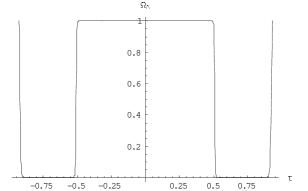
Figure 1: Plot of the vacuum density parameter $\Omega_{\Lambda}$ as a continuous function of dimensionless parameter time $\tau$ for $\tau\in\left[-0.930352,0.930352\right]$. The initial inflation ($\tau=0$) and the final de Sitter stage appear. The function $\Omega_{\Lambda}(\tau)$ was parametrized by the interpolating functions $y(\tau)$ and $h(\tau)$, and the numerical solutions of Eq. (30) and (31) with the initial conditions (40) and (41).

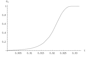
Figure 2: Plot of $\Omega_{\Lambda}$ versus $\tau$ at the end of the evolution. The universe enters again on a phase of acceleration for $\Omega_{\Lambda}>1/3$ and tends to de Sitter (plateau $\Omega_{\Lambda}=1$). The present time $\tau_{0}=0,9220725$ i.e. $t_{0}=4,88.10^{17}\,s$ corresponds to $\Omega_{\Lambda 0}=0.63$ (see table 1).

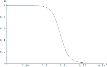
Figure 3: Plot of $\Omega_{\Lambda}$ versus $\tau$ at the beginning of the evolution. There is an initial inflation (de Sitter $\Omega_{\Lambda}=1$), then a graceful exit of inflation for $\Omega_{\Lambda}<1/3$ (see table 1).

As the current values of the observational data ($\Omega_{\Lambda}(\tau_{0})=0.7$ , $H(\tau_{0})=72$ $kms^{-1}Mpc^{-1}$) of the $\Lambda CDM$ model [37][38] are model-dependent, we use the values derived in the framework of our $\Lambda(t)CDM$ model from the studies of SnIa observational constraints [14]

$$\Omega_{\Lambda}(\tau_{0})=0.63\text{ , }H(\tau_{0})=64\text{ }kms^{-1}Mpc^{-1}\text{ ,}$$ (42)

where $\tau_{0}$ represents the present instant. Let us emphasize that the use of the values derived from the $\Lambda CDM$ concordance model would only marginally modify the following results.

The different scales $H_{1}$,$Y_{1}$, and $\Lambda_{1}$ can be deduced from these two values (42). We deduce the instant $\tau_{0}$ from the plot of the function $\Omega(\tau)$

$$\tau_{0}=0.9220725\text{ .}$$ (43)

Setting this value in $y(\tau)$ and $h(\tau)$ and using (35), we deduce

$$y(\tau_{0})=2.0576\times 10^{18}\text{ , }h(\tau_{0})=5.7149\times 10^{7}\text{ , }\lambda(\tau_{0})=2.0576\times 10^{18}\text{ .}$$ (44)

Then, Eq. (28) with the numerical values (42) and (44) yields

$$H_{1}=\frac{H(\tau_{0})}{h(\tau_{0})}=3.62928\times 10^{-26}s^{-1}\text{ .}$$ (45)

From (32), (41) and (45), we have

$$Y_{1}=\frac{X_{1}H_{1}^{2}}{c^{2}}=1.46555\times 10^{-71}m^{-2}\text{.}$$ (46)

Besides, $\Lambda(\tau_{0})$ is directly fixed by the observational data (42) from (38)

$$\Lambda(\tau_{0})=\frac{3\Omega_{\Lambda}(\tau_{0})H^{2}(\tau_{0})}{c^{2}}=9.04649\times 10^{-53}m^{-2}\text{ .}$$ (47)

Thus with (34) and (44)

$$\Lambda_{1}=\frac{\Lambda(\tau_{0})}{\lambda(\tau_{0})}=4.39662\times 10^{-71}m^{-2}\text{.}$$ (48)

The numerical value of $r_{1}$ linked to the scale $Y_{1}$ and identified to the value $L_{1}$ of Eq. (20) can now be estimated from (33), (41) and (46): $r_{1}=8.26037\times 10^{7}m$. It is an intermediary scale between $L_{P}\simeq 8.02121\times 10^{-35}m$ (for $l_{P}^{\prime}:=\sqrt{\frac{\text{h{\hskip-1.39998pt}\hbox to0.0pt{\hss\rule[3.31529pt]{2.27498pt}{0.3014pt}}{\hskip 1.39998pt}}G}{c^{3}}}\simeq 1.6\times 10^{-35}m$, with $L_{P}=2\sqrt{2\pi}l_{P}^{\prime}$ ) and $L_{\Lambda today}=r(\tau_{0})\simeq 1.82104\times 10^{26}m$. We then obtain

$$\frac{\Lambda(0)}{\Lambda(\tau_{0})}=\frac{y(0)(1+\alpha_{1}y(0))}{y(\tau_{0})(1+\alpha_{1}y(\tau_{0}))}\simeq 4.86003\times 10^{112}\text{ .}$$ (49)

The dark energy density parameter $\Omega_{\Lambda}(\tau)$ decreases from the initial value $\Omega_{\Lambda}(0)=1$ and then reaches the value $1/3$, i.e. the end of the acceleration (or equivalently the exit of inflation), which occurs at the instant $t_{2}=1.23824\times 10^{-39}s$ (evaluated from Eq. (29)).

Then, it passes through a minimum $\Omega_{\Lambda m}(\tau_{m})=4.99970\times 10^{-20}$ at the instant $t_{m}=2.9042\times 10^{-11}s$ where $\Lambda(\tau_{m})=8.795\times 10^{-16}m^{-2}$ and $H(\tau_{m})=2.2955\times 10^{10}s^{-1}$. After, $\Omega_{\Lambda}(\tau)$ increases again ( $\Lambda$ comes back [Krauss and Turner 1995 34b]) until a return of the inflation which occurs at the instant $t_{3}=1.81\times 10^{17}s=5.73\,Gyr$ .

It reaches its present day value $0.63$ at $\tau_{0}$ (43) or $t_{0}=4.88084\times 10^{17}s=15.4664Gyr$. This value is in good agreement with the observational results derived from the “concordance model” ([38] Section 2.5. p.3) and allows to avoid the age crisis (see e.g. [39]). With a linear extrapolation of $H(\tau)$ during $\tau_{3}-\tau_{0}$, we roughly evaluate the redshift, namely $z(\tau_{3})\simeq 1.01826$, where the acceleration begins again. This value is in good agreement up to the previous approximation with the exact value of the transition redshift $z_{T}=0.965$ found in [14].

In the same time, the “coincidence problem” is resolved. The date of the coincidence can be defined by different ways : for instance by the instant $t_{m}$ (see above), i.e. the instant from which $\Omega_{\Lambda}$ grows again, or by the instant $t_{3}$ (see above) when the universe inflates again, or even, more recently, by the instant $t_{4}=3.61505\times 10^{17}s=11.4554Gyr$ when $\Omega_{\Lambda}=\frac{1}{2}=\Omega_{m}$. In the following, we use this last definition.

If we admit that the recombination starts at the instant $t_{\ast}=1.17\times 10^{13}s=372kyr$, and ends at $t_{\ast}^{\prime}=1.54\times 10^{13}s=487kyr$ , the values of the main cosmological parameters are, for these instants : $\Omega_{\Lambda}(\tau_{\ast})=1.43\times 10^{-4}$, $\Omega_{\Lambda}(\tau_{\ast}^{{}^{\prime}})=1.722\times 10^{-4}$, $H(\tau_{\ast})=5.68\times 10^{-14}s^{-1}$, $H(\tau_{\ast}^{\prime})=4.34\times 10^{-14}s^{-1}$, $\Lambda(\tau_{\ast})=1.54\times 10^{-47}m^{-2}$, $\Lambda(\tau_{\ast}^{\prime})=1.08\times 10^{-47}m^{-2}$. A determination of the value of $\Omega_{\Lambda}(\tau_{\ast}^{{}^{\prime}})$ ( or of $\Omega_{m}(\tau_{\ast}^{{}^{\prime}})$ ) from observational data, if feasible, would be an interesting test for the model. The following table presents the main results of the FLRW e.h. model.

$\tau$	$t(s)$	$H(s^{-1})$	$\Omega_{\Lambda}$	$\Lambda(m^{-2})$
$0$	$0$	$4.574$ $10^{38}$	$1$	$6.98$ $10^{60}$
$\tau_{2}=0.50993$	$t_{2}=1.24$ $10^{-39}$	$2.79$ $10^{38}$	$0.333$	$8.685$ $10^{59}$
$\tau_{m}=0.6862$	$t_{m}=2.90$ $10^{-11}$	$2.29$ $10^{10}$	$5$ $10^{-20}$	$8.795$ $10^{-16}$
$\tau_{\ast}=0.8786$	$t_{\ast}=1.17$ $10^{13}$	$5.68$ $10^{-14}$	$1.43$ $10^{-4}$	$1.542$ $10^{-47}$
$\tau_{\ast}^{\prime}=0.8796$	$t_{\ast}^{\prime}=1.537$ $10^{13}$	$4.34$ $10^{-14}$	$1.72$ $10^{-4}$	$1.082$ $10^{-47}$
$\tau_{3}=0.9189$	$t_{3}=2.29$ $10^{17}$	$3.52$ $10^{-18}$	$0.333$	$1.378$ $10^{-52}$
$\tau_{4}=0.92081$	$t_{4}=2.87$ $10^{17}$	$3.15$ $10^{-18}$	$0.5$	$1.655$ $10^{-52}$
$\tau_{0}=0.92207$	$t_{0}=4.88$ $10^{17}$	$2.07$ $10^{-18}$	$0.63$	$9.046$ $10^{-53}$

Table1. Values of $H$ , $\Omega_{\Lambda}$ and $\Lambda$ at some key times of the evolution.

The long period about from $6.39\times 10^{-40}s$ to $t_{4}\simeq 2.8\times 10^{17}s$ when $\Lambda$ does not dominate, i.e. when $\Omega_{\Lambda}<0.5$, allows to maintain the standard model and its afferent results all along this period.

Another interesting result to be noted is the shape of the curve $\Omega_{\Lambda}(\tau)$ ( fig.1) which presents a symmetry with respect to $\tau=0$ , suggesting a period for $\Omega_{\Lambda}(\tau)$. Each curve ( $\Omega_{\Lambda},h,y,\lambda,H,\Lambda$) is (quasi-) symmetrical with respect to $t=0$. The functions $\Lambda(\tau)$ and $H(t)$ decrease (increase resp.) when $\tau\geq 0$ ($\tau\leq 0$ resp.). There is a “big bounce” on an inflationary space at $t=0$, with a period that is stretched over more than twice $t_{0}$ and another one at a very large time on a quasi- de Sitter space. We studied above the results given for $\tau\geq 0$ only. The first inflation is “strong” (at $t=0$) when $\Lambda$ is maximum, the second one is “weak”(at $t\rightarrow\infty$) when $\Lambda$ is minimum (possibly$\rightarrow 0$). Today, $\Lambda$ is on the way to its minimum (maybe zero), and the universe is dominated by the small cosmological constant (37).

We can also obtain the $R(t)$ ( or “jerk” $j(t)$ ) and $S(t)$ “statefinder” parameters [40] and $q(t)$ deceleration parameter for the model

$$q\equiv\frac{-\overset{\cdot\cdot}{a}}{aH^{2}}=-1+\frac{3\gamma}{2}(1-\Omega_{\Lambda})$$ (50)

$$R\equiv\frac{\overset{\cdot\cdot\cdot}{a}}{aH^{3}}=3X_{1}\frac{y(1+2\alpha_{1}y)}{h^{3}}(\sqrt{X_{1}y}-h)+1$$ (51)

$$S\equiv\frac{R-1}{3(q-\frac{1}{2})}\text{ ,}$$ (52)

with for their present day values

$$q_{0}=-0.445\text{ , }R_{0}=0.610125\text{, }S_{0}=0.137522\text{ .}$$ (53)

The positive sign of $R_{0}$ indicates the present overinflation, (either increasing of inflation, or trend towards inflation). One can also evaluate $R$ in the early period of deflation (i.e. desinflation). For instance at $\tau=0.509275$ when inflation was present, though decreasing, because $\Omega_{\Lambda}(\tau=0.509275)=0.4>\frac{1}{3}$, we obtain $R(\tau=0.509275)=-1.414<0$.We can yet obtain $R<0$ for $\Omega_{\Lambda}<\frac{1}{3}$ during some time after the end of the initial inflation. For example at $\tau=0.51151$ when $\Omega_{\Lambda}=0.2<\frac{1}{3}$, we have yet $R(\tau=0.51151)=-0.20005$. The instant when $R$ changes of sign is given by $\tau_{9}=0.51204075$ or $t_{9}=3.07026\times 10^{-39}s$. Since then, $R$ is positive.

The comparison of the “kinematical” values (53) to observations (SNAP supernova data ) could also be a test for our model (see the remark of [40], Section 4) and would allow the measurement of the production source of CDM [41] which is constrained by the statefinder parameters and the “snap” parameter $s:=\frac{\overset{(4)}{a}}{aH^{4}}$.

Finally, this model also supports the low-$l$ CMBR power spectrum suppression suspected in the WMAP data. Indeed, the event horizon plays naturally the role of a dynamical IR cut-off translatable to a wave number cutoff [42] [43] as for the holographic model [25] [30]. Applying the same procedure as [42] [43] for the Dirichlet boundary condition $\lambda_{c}=2r_{0}$, we roughly evaluate the influence of this cutoff. In the integrated Sachs-Wolfe (ISW) effect, the IR cutoff appears as the lower limit of the comoving momentum which truncates the summation giving the coefficient $C_{l}$ of the power spectrum. For a power law spectrum with a spectral index $n=1$ (Harrisson-Zeldovich), we have for the low $l$ [42]:

$$C_{l}\simeq N\sum_{k>k_{c}}\frac{1}{k}j_{l}^{2}(k\eta_{0})$$ (54)

where $j_{l}$ are the spherical Bessel functions. In flat spacetime, the multipole number $l$ is given by

$$l=k_{l}(\eta_{0}-\eta^{\ast})$$ (55)

where $(\eta_{0}-\eta^{\ast})$ is the comoving distance to the last scattering surface.The definition of the conformal time in flat space $\eta=-\frac{r}{a}$ with the Dirichlet limits condition leads to

$$l_{c}=\pi((1+z^{\ast})\frac{r^{\ast}}{r_{0}}-1)\text{.}$$ (56)

Taking the current value $z^{\ast}=1089$ [5, 44] and using (18), we obtain

$$r=\sqrt{\frac{3}{2\Lambda}(1+\sqrt{1+\frac{4}{3}\alpha\Lambda})}\text{ .}$$ (57)

$\frac{r^{\ast}}{r_{0}}$ can be evaluated with $\Lambda^{\ast}$and $\Lambda_{0}$ from Table 1 and we find : $l_{c}=5.15$. For the value $\Lambda^{\prime\ast}$ of the end of the recombinaison, we get : $l_{c}^{\prime}=6.76$. These values are in the expected range.

7 Conclusion

From the FLRW e.h. entropy with thermal fluctuations (Eq. (14)), we obtained the corresponding law for the cosmological constant $\Lambda(r)$ as a function of the event horizon radius $r$ (Eq. (18)). We used the striking similarity of this last expression (18) with a renormalization relation (Eq. (20)) to reinterpret (18) in terms of such a (truncated) renormalization relation (20).

Using this $\Lambda(r)$ law in an interacting two-component $\Lambda(t)CDM$ cosmological model in a FLRW spacetime, we derived a system of coupled equations for $H(t)$ and $r(t)$ (Eqs. (30) and (31)). Through a numerical resolution (Section 6), we obtained the curves of evolution of $\Omega_{\Lambda}$ (figs. 1 to 3), the table 1 of the values of the main cosmological parameters ($H,\Omega_{\Lambda}$) at different times in the evolution of the universe, and the evolution of the deceleration and statefinder parameters.

The event horizon thermodynamical model presented here allows us to account for most of essential features of the cosmology such as the value of the age of the universe,$\sim 15.5Gyr$ (safe from the age problem [45]), the ratio $\frac{\Lambda[0]}{\Lambda[\tau_{0}]}\sim 5\times 10^{112}$, as well as the exit of inflation after about $t_{2}\simeq 23000$ Planck times, the existence of a minimum $\sim 5$ $\times 10^{-20}$ for $\Omega_{\Lambda}$ attained after about $3$ $\times 10^{-11}s$, the coming back of the inflation (after about $7.24Gyr$ from the beginning), followed by the recent coincidence, at $11.4Gyr$, with the matter density, but also allows us to address the entropy problem, and the creation of (dark) matter from the vacuum energy. Besides, the model does not perturb the results of the old standard model for the period going from $6.39\times 10^{-40}s$$\simeq 10000$ Planck times to $2.87\times 10^{17}s=11.4Gyr$ all along which the DE is subdominant ( $\Omega_{\Lambda}<0.5$ ). Finally, it can render an account of the low-$l$ CMBR power spectrum suppression, for an angular scale corresponding to multipole numbers lower than $l_{c}\sim 7$.

References

- [1] Riess AG et al., 1998 Astron. J. 116 1009
- [2] Perlmutter S et al., 1998 Nature 391 51
- [3] Weinberg S, 1989 Rev. Mod. Phys. 61 1
- [4] Padmanahban T, 2000 [astro-ph/0204020]
- [5] Bennett CL et al., 2003 [astro-ph/0302207]
- [6] Freedman W L et al., 2001 ApJ 583 47
- [7] White DH and Fabian AC, 1995 MNRAS 273 73
- [8] Yokoyama J, 2003 [gr-qc/0305068]
- [9] Ratra B and Peebles PJ E, 1988 Phys.Rev.D 37 3406
- [10] Caldwell RR, Dave R and Steinhardt PJ, 1998 Phys. Rev.Lett. 80 1582
- [11] Murphy G L,1973 Phys.Rev.D8 4231
- [12] Overduin JM and Cooperstock FI, 1998 Phys.Rev.D 58 043506
- [13] Gariel J and Le Denmat G, 1999 Class.Quantum Grav.16 149
- [14] Gariel J, Le Denmat G and Barbachoux C, 2005 Phys.Lett. B 629 1 [astro-ph/0507318 ]
- [15] Gibbons G and Hawking S W, 1977 Phys.Rev.D 15 2738
- [16] Pollock MD and Singh TP, 1989 Class.Quantum Grav.6 901
- [17] Srivastava S K, [astro-ph/0602116].
- [18] Das S , Majumdar P and Bhaduri RK, 2002 Class.Quantum Grav.19 2355
- [19] Davies PCW and Davis TM, 2002 Found.ofPhys. 32 1877
- [20] Cartan E, 1922 Journ.Math.Pure Appl. 1 141
- [21] Ishak M, 2005 [astro-ph/0504416]
- [22] Pavon D, Sen S and Zimdhal W, 2004 [astro-ph/0402067]
- [23] Zimdhal W and Pavon D, 2004 GRG 36 1483
- [24] Gasperini M, 1988 Class.Quantum Grav. 5 521
- [25] Li M, 2004 Phys. Lett. B603 1
- [26] Cohen A G, Kaplan DB and Nelson AE, 1999 Phys. Rev. Lett. 82 4971
- [27] Thomas S, 2002 Phys.Rev.Lett. 89081301
- [28] Fischler W and Susskind L, 1998 [hep-th/9806039]
- [29] Hsu S D H, 2004 [hep-th/0403052]
- [30] Huang QG and Gong Y, 2004 J.Cosmol.Astropart.Phys. JCAP08(2004)006
- [31] Major S A and Setter K L, 2001 gr-qc/0101031 [gr-qc/0108034]
- [32] Shapiro I, Sola J and Stefancic H, 2005 J.Cosmol.Astropart.Phys. JCAP01(2005)012
- [33] Babic A, Guberina B, Horvath R and Stefancic H, 2005 [astro-ph/0407572]
- [34] F. Bauer, 2005 [gr-qc/051200702]
- [35] Padmanabhan T, 2004 [astro-ph/0411044]
- [36] Myung Y S, 2005 Phys. Lett. B 610 18
- [37] Freedman W L and Turner M, 2003 Rev.Mod.Phys.75 1433
- [38] Tegmark M et al., 2003 [astro-ph/0310723]
- [39] Primack J R, 2004 [astro-ph/0408359]
- [40] Alam U, Sahni V, Saini T D and Starobinsky A A, 2003 [astro-ph/0303009]
- [41] Szydlowski M, 2005 [astro-ph/050234v2]
- [42] Enqvist K and Sloth M S, 2004 Phys. Rev. Lett. 93 221302
- [43] Enqvist K, Hannestad S and Sloth M S, 2005 J.Cosmol. Astropart. Phys. JCAP02(2005)004
- [44] Spergel D N et al., 2003 [astro-ph/0302209]
- [45] Krauss L M and Turner M S, 1995 GRG 27 1137