The Effect of Large-Scale Structure on the SDSS Galaxy Three–Point Correlation Function

Abstract

We present measurements of the normalised redshift–space three–point correlation function ($Q_{z}$) of galaxies from the Sloan Digital Sky Survey (SDSS) main galaxy sample. These measurements were possible because of a fast new N–point correlation function algorithm (called npt) based on multi–resolutional k-d trees. We have applied npt to both a volume–limited (36738 galaxies with $0.05\leq z\leq 0.095$ and $-23\leq{M_{{}^{0.0}r}}\leq-20.5$) and magnitude–limited sample (134741 galaxies over $0.05\leq z\leq 0.17$ and $\sim M^{*}\pm 1.5$) of SDSS galaxies, and find consistent results between the two samples, thus confirming the weak luminosity dependence of $Q_{z}$ recently seen by other authors. We compare our results to other $Q_{z}$ measurements in the literature and find it to be consistent within the full jack–knife error estimates. However, we find these errors are significantly increased by the presence of the “Sloan Great Wall” (at $z\sim 0.08$) within these two SDSS datasets, which changes the 3–point correlation function (3PCF) by 70% on large scales ($s\geq 10h^{-1}$ Mpc). If we exclude this supercluster, our observed $Q_{z}$ is in better agreement with that obtained from the 2dFGRS by other authors, thus demonstrating the sensitivity of these higher–order correlation functions to large–scale structures in the Universe. This analysis highlights that the SDSS datasets used here are not “fair samples” of the Universe for the estimation of higher–order clustering statistics and larger volumes are required. We study the shape–dependence of $Q_{z}(s,q,\theta)$ as one expects this measurement to depend on scale if the large scale structure in the Universe has grown via gravitational instability from Gaussian initial conditions. On small scales ($s\leq 6h^{-1}$ Mpc), we see some evidence for shape–dependence in $Q_{z}$, but at present our measurements are consistent with a constant within the errors ($Q_{z}\simeq 0.75\pm 0.05$). On scales $>10h^{-1}$ Mpc, we see considerable shape–dependence in $Q_{z}$. However, larger samples are required to improve the statistical significance of these measurements on all scales.

1 Introduction

Correlation functions are some of the most commonly used statistics in cosmology. They have a long history in quantifying the clustering of galaxies in the Universe (see Peebles 1980). There is a hierarchy of correlation functions. The two–point correlation function (2PCF) compares the number of pairs of data points, as a function of separation, with that expected from a Poisson distribution. Next in the hierarchy is the 3–point correlation function (3PCF), which compares the number of data triplets, as a function of their triangular–configuration, to that expected from Poisson. Higher-order correlations are defined analogously.

As discussed by many authors, the higher–order correlation functions contain a variety of important cosmological information, which complements that from the 2PCF (Groth, & Peebles, 1977; Balian & Schaeffer, 1989). These include tests of Gaussianity and the determination of galaxy bias as a function of scale (Suto, 1993; Jing & Börner, 1998; Takada & Jain, 2003; Jing & Börner, 2004; Kayo et al., 2004; Lahav & Suto, 2004). Such tests can also be performed using the Fourier-space equivalent of the 3PCF, the bi-spectrum (Peebles, 1980; Scoccimarro et al., 1999, 2001; Verde et al., 2002) or other statistics such as the void probability distribution and Minkowski functionals(Mecke et al., 1994). Recent results from these complementary statistics using the SDSS main galaxy sample include Hikage et al. (2002, 2003, 2005) and Park et al. (2005).

While the 3PCF is easier to correct for survey edge effects than these other statistics, measurements of the 3PCF have been limited by the availability of large redshift surveys of galaxies (see Szapudi, Meiksin & Nichol 1996, Frieman & Gaztanaga 1999, Szapudi et al. 2002 for 3PCF analyses of large solid angle catalogues of galaxies) and the potentially prohibitive computational time needed to count all possible triplets of galaxies (naively, this count scales as $O(N^{3})$, where $N$ is the number of galaxies in the sample).

In this paper, we resolve these two problems through the application of a new N–point correlation function algorithm (Moore et al., 2001) to the galaxy data of the Sloan Digital Sky Survey (SDSS; York et al. 2000). We present herein measurements of the 3PCF from the SDSS main galaxy sample. Our measurements illustrate the sensitivity of the 3PCF to known large-scale structures in the SDSS (Gott et al., 2005). They are complementary to the work of Kayo et al. (2004) who explicitly explored the luminosity and morphological dependence of the 3PCF using SDSS volume–limited galaxy samples. These measurements of the 3PCF will help facilitate constraints on the biasing of galaxies and will aid in the development of theoretical predictions for the higher–order correlation functions (Scoccimarro et al., 2001; Takada & Jain, 2003). Throughout this paper, we use the dimensionless Hubble constant $h\equiv H_{\rm 0}/100\,{\rm km\,s^{-1}\,Mpc^{-1}}$, the matter density parameter $\Omega_{\rm m}=0.3$, and the dimensionless cosmological constant $\Omega_{\Lambda}=0.7$, unless stated otherwise.

2 The 3PCF Computational Algorithm

To facilitate the rapid calculation of the higher–order correlation functions, we have designed and implemented a new N–point correlation function (NPCF) algorithm based on k-d trees, which are multi–dimensional binary search tree for points in a k-dimensional space. The k-d tree is composed of a series of inter–connected nodes, which are created by recursively splitting each node along its longest dimension, thus creating two smaller child nodes. This recursive splitting is stopped when a pre-determined number of data points is reached in each node (we used $\leq 20$ data points herein). For our NPCF algorithm, we used an enhanced version of the k-d tree technology, namely multi–resolutional k-d trees with cached statistics (mrkdtree), which store additional statistical information about the search tree, and the data points in each node, e.g., we store the total count and centroid of all data in each node.

The key to our NPCF algorithm is to use multiple mrkdtrees together, and store them in main memory of the computer (rather than on disk), to represent the required N–point function, e.g., we use 3 mrkdtrees to compute the 3PCF, 4 mrkdtrees for the 4PCF, and so on. The computational efficiency is increased by pruning these trees wherever possible, and by using the cached statistics on the tree as much as possible. The details of mrkdtrees and our NPCF algorithm (known as npt) have already been outlined in several papers (Moore et al., 2001; Nichol et al., 2003; Gray et al., 2004). Similar tree–based computational algorithms have been discussed by Szapudi et al. (2001).

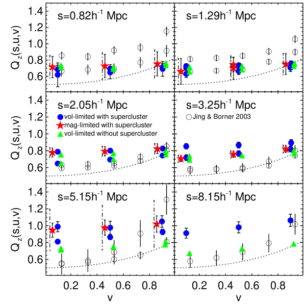
Figure 1: Our SDSS measurements of the normalised redshift–space 3PCF as a function of triangle configuration, i.e., $Q_{z}(s,u,v)$. We compare our measurement with that of Jing & Börner (1998, 2004) for both the 2dFGRS (open circles and error bars) and LCRS (dashed line) galaxy surveys. These two estimates of $Q_{z}(s,u,v)$ do not agree because of the different passbands used for these two surveys. We also provide two values of $u$ (namely $u=1.29$ and $u=3.04$) from the Jing & Börner (2004) data, i.e., we have not plotted the $u=2.09$ data to avoid over-crowding. The binning has been chosen to be identical to that of Jing & Börner (2004). The solid (blue) circles are the SDSS $Q_{z}$ for the volume–limited sample as discussed in Section 3, while the solid (red) star symbols are the SDSS $Q_{z}$ for the SDSS magnitude limited sample. The solid error bars shown on these data–points are estimated using jack–knife re–sampling (see text), but with sub–regions 3 and 4 in Figure 2 removed (i.e., excluding the supercluster from these error bars). For comparison, the dot–dashed error bars on the red star symbols are our estimate of the jack–knife errors (the diagonal elements of the covariance matrix) using all 14 sub–regions to estimate the error (i.e., the effect of the supercluster is now including in the size of the error bar). In some cases, the error bars are smaller than the plotting symbols. The solid (green) triangle symbols are the SDSS $Q_{z}$ for the jack–knife re–sample excluding sub–regions 3 and 4

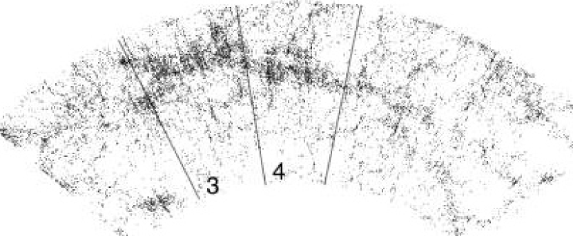
Figure 2: Part of the SDSS volume–limited sample defined in Section 3. This redshift slice is approximately 500 by 200 $h^{-1}$ Mpc in the dimensions shown, and $\sim 100h^{-1}$ Mpc thick (although here we have collapsed the slice in this $3^{rd}$ dimension). Most noticeable is the supercluster, which has been called the “Sloan Great Wall” by Gott et al. (2005) and is 1.37 billion light years long. This supercluster is a combination of the Leo A and SCL126 superclusters (Einasto et al. 2001), and is associated with tens of known Abell clusters of galaxies. The two regions labelled 3 and 4 are two of the 14 sub–regions used in deriving the covariance matrices on our correlation functions as shown as error bars in Figure 1.

Figure 3: (Left) The percentage difference between the 2PCFs for the 14 SDSS jack–knife datasets and the 2PCF as measured for the whole dataset (without any sub–regions excluded). The open stars are for the 12 jack–knife datasets with the supercluster shown in Figure 2 included, while solid triangles are for the dataset with sub–region 4 excluded (Figure 2) and solid circles are for the dataset with sub–region 3 excluded. (Right) The percentage difference between the 3PCFs for the 14 SDSS jack–knife datasets and the 3PCF as measured for the whole dataset. The x-axis ($S_{12}$) is the redshift–space distance for the shortest side of the triangle (see Eqn 2).The open stars are for jack–knife datasets with the supercluster shown in Figure 2 included, while solid triangles are for the dataset with sub–region 4 excluded (Figure 2) and solid circles are for the dataset with sub–region 3 excluded. All triangle configurations are plotted here, i.e., one point per triangle configuration in Figure 1, which explains why there are many data points with the same values of $s$ and $s_{12}$.

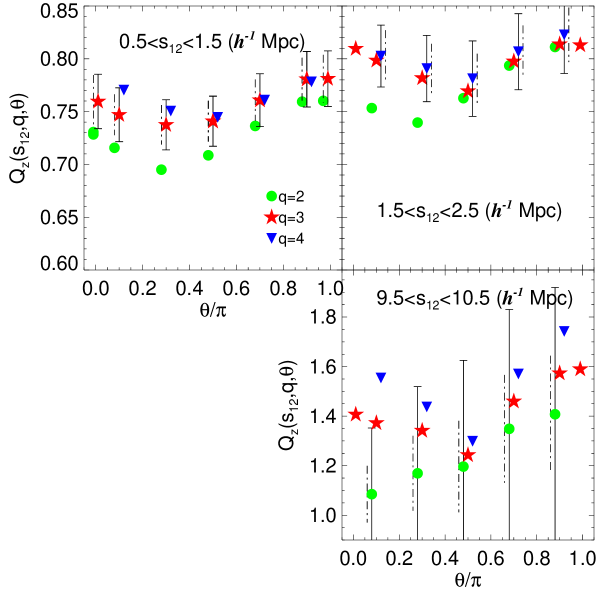
Figure 4: The SDSS $Q_{z}$ as a function of $\theta$, $q$ and $s_{12}$ for the Pope et al. sample discussed in the text. We show 3 bins in $s_{12}$ (as labeled), while $\theta$ is given in radians along the x-axis (bin width of $\Delta\theta\pm 0.05$ radians about the central value plotted). The solid (green) circles are for $q=2$, solid (red) stars are for $q=3$ and the solid (blue) triangles are for $q=4$ ($\Delta q\pm 0.5$ about the central value). We also include a set of data points at the extremes of the $\theta$ range, specifically $0.0<\theta<0.02$ and $0.98<\theta<1.00$. The $q=2$ and $q=4$ data points are offset by $-0.02$ and $+0.02$ radians respectively to reduce overcrowding. Likewise, we only plot the full error bars (solid lines) on a fraction of the data points. The dot-dashed error bars have been calculated with sub–regions 3 and 4 omitted (see Figure 2).

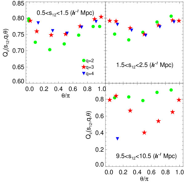
Figure 5: The same as Figure 4 but now with sub–region 3 omitted from the calculation of $Q_{z}(s_{12},q,\theta)$ for the Pope et al. (2004) sample. We have not plotted error bars.

3 SDSS Data

The details of the SDSS survey are given in a series of technical papers by Fukugita et al. (1996); Gunn et al. (1998); York et al. (2000); Hogg et al. (2001); Strauss et al. (2002); Smith et al. (2002); Pier et al. (2003); Blanton et al. (2003b); Ivezic et al. (2004); Abazajian et al. (2005). For the computations discussed herein, we use two SDSS catalogues. The first is a volume–limited sample of 36738 galaxies in the redshift range of $0.05\leq z\leq 0.095$ and absolute magnitude range of $-23\leq{M_{{}^{0.0}r}}\leq-20.5$ (for $h=0.7$ and the $z=0.0$ SDSS $r$ filter, or ${}^{0.0}r$ in Blanton et al. (2003b) terminology), covering 2364 deg² of the SDSS photometric survey. All the magnitudes were reddening corrected using Schlegel, Finkbbeiner, & Davis (1998), and the k-corrected v1_16 software (Blanton et al., 2003b). The second sample is the same as “Sample 12” used by Pope et al. (2004) and contains 134741 galaxies over 2406 deg². This latter sample is not volume–limited, but is constrained to the absolute magnitude range of $-22\leq{M_{{}^{0.1}r}}\leq-19$ (or $M^{*}\pm 1.5$ magnitudes) for $h=1$, and using the $z=0.1$ SDSS r filter system, or ${}^{0.1}r$ (Blanton et al., 2003b; Zehavi et al., 2005). To compare the two samples, our volume–limited sample has the absolute magnitude range of $-23.54\leq{M_{{}^{0.1}r}}\leq-21.04$ in the same ${}^{0.1}r$ filter as used for the Pope et al. sample; assuming a conversion of ${{}^{0.1}}r\simeq{{}^{0.0}}r+0.23$ for the SDSS main galaxy sample with a median color at $z=0.0$ of ${{}^{0.0}}(g-r)\simeq 0.8$. This gives a mean space density of $8.25\times 10^{-3}\,h^{3}$ Mpc^-3, which is comparable to the space densities of the SDSS main galaxy sample given in Table 2 of Zehavi et al. (2005).

We have made no correction for missing galaxies due to fibre–collisions (i.e., two SDSS fibres can not be placed closer than 55 arcseconds on the sky). We do not expect this observational constraint to bias our correlation functions as the adaptive tilting of SDSS spectroscopic plates reduces the problem to $\simeq 7\%$ of possible target galaxies being missed (see Blanton et al. 2003a for details). Furthermore, this bias will only affect pairs of galaxies separated by less than 100$h^{-1}$ kpc, which is significantly smaller than the scales studied herein. In each case, we also constructed catalogues of random data points (containing $8\times 10^{5}$ points) over the same area of the sky and with the same selection function as discussed in Pope et al. (2004). These random catalogues are then used to calculate edge effects on the N–point correlation functions using the estimators presented in Szapudi & Szalay (1998).

4 Results

There are two common parametrizations of $Q_{z}$. One defines

$$s=s_{12},\quad u=\frac{s_{23}}{s_{12}},\quad{\rm and}\quad v=\frac{s_{31}-s_{23}}{s_{12}},$$ (1)

where $s_{12}$, $s_{23}$ and $s_{31}$ are the three sides of a triangle in redshift space. Then $Q(s,u,v)$ is defined by the ratio of the 3PCF $\zeta(s_{12},s_{23},s_{31})$, to sums of products of 2PCFs (e.g. $\xi(s_{12})\xi(s_{13})$ and permutations):

$$Q_{z}(s,u,v)\equiv\frac{\zeta(s_{12},s_{23},s_{31})}{\xi(s_{12})\xi(s_{23})+\xi(s_{23})\xi(s_{31})+\xi(s_{31})\xi(s_{12})}.$$ (2)

The second parametrization has $Q_{z}(s,q,\theta)$ with $s=s_{12}$ being the shortest side of the redshift-space triangle, $q=s_{23}/s_{12}$, and $\theta$ the angle between these two sides ($s_{12}$ and $s_{23}$).

Figure 1 shows $Q_{z}(s,u,v)$ for both our volume–limited sample (filled circles) and the Pope et al. (2004) sample (filled stars). Different panels show results for a range of triangle configurations. To facilitate a direct comparison with results from the literature, we have used the same binning scheme as Jing & Börner (1998, 2004), in their analyses of the Las Campanas Redshift Survey (LCRS) and 2dF Galaxy Redshift Survey (2dFGRS). The open circles show their results. Overall, our $Q_{z}(s,u,v)$ values are consistent with theirs, but with some obvious disagreements. For example, on large scales ($s_{12}>10h^{-1}{\rm Mpc}$), we find larger $Q_{z}\sim 1$, while Jing & Börner (2004) find much smaller values. Although the different selection passbands of the 2dFGRS ($b_{j}$) and SDSS ($r-$band) might account for this difference, it cannot account for the disagreement with the LCRS measurements of Jing & Börner (1998) since the LCRS was also $r$–band selected.

To quantify the disagreement, we estimated the covariances of our 3PCF estimates using the jack–knife re–sampling technique (discussed in detail in Scranton et al. (2002) and Zehavi et al. (2002, 2005)). Briefly, the jack-knife resampling technique provides an estimate of the “cosmic variance” within a sample. It is calculated by splitting the dataset into sub–regions and then measuring the variance seen between the estimated correlation functions as sub–regions are omitted one-by-one (therefore, if there are $N$ subregions, there are $N$ correlation function estimates). As shown in Figure 2 of Zehavi et al. (2005), the jack-knife errors accurately reproduce the “true error” (the dispersion measured between 100 mock galaxy catalogues), especially for the diagonal terms of the covariance matrix of the 2PCF on large scales, (for $r>0.5h^{-1}$Mpc, the difference between the two error estimates is always $<10\%$). In what follows, we assume that the jack-knife error estimates are also accurate for the 3PCF.

The SDSS dataset is built-up of thin “wedge-shaped” regions that are 2.5 degrees thick in declination and hundreds of degrees wide in right ascension (see York et al. 2000). We divided the total volume of our volume limited catalogue up into 14 sub–regions when estimating the covariance matrix. These were selected in Right Ascension along the SDSS scans. To illustrate, Figure 2 shows one of the redshift wedges; two of the sub–regions (namely sub–regions 3 and 4) are highlighted to provide an impression of the typical size of a subregion, but also because these two particular regions will feature prominently in what follows.

The error bars shown in Figure 1 show the diagonal elements of the covariance matrices we estimate from the jack-knife method. The sizes of these diagonal elements (as well as the off–diagonal elements) are extremely sensitive to the inclusion or exclusion of sub–regions 3 and 4. This sensitivity is quantified in Figure 3 which shows the scatter between the 14 2PCFs and 3PCFs used to construct the covariance matrices. The scatter in the 2PCFs between 12 of the 14 jack–knife datasets, which contain the supercluster seen in Figure 2, is less than 10% on all scales probed herein ($s\leq 40\,h^{-1}$ Mpc) which is consistent with the findings of Zehavi et al. (2005). The 2 datasets which exclude sub–regions 3 and 4, have significantly different 2PCFs, up to 40% different on the largest scales, which is again consistent with Zehavi et al. (2005) who find that this supercluster greatly affects their 2PCF on large scales and is not accounted for by their estimates of the jack–knife errors. The effect on the 3PCF of the “Sloan Great Wall” is much greater. The jack–knife datasets that exclude sub–regions 3 and 4 (which contain the supercluster) differ by up to 70% (on large scales) compared to all other 3PCFs.

In Figure 1, we show the normalised 3PCF $Q_{z}$ for the whole dataset as well as for the datasets with sub–regions 3 and 4 excluded. With the bulk of this supercluster excluded, the SDSS 3PCF has much lower $Q_{z}(s,u,v)$ values on large scales and is now in good agreement with the Jing & Börner (2004) 2dFGRS 3PCF on these large scales. This is also demonstrated in the error bars shown in Figure 1 which were estimated using all 14 jack–knife datasets (dot–dashed error bars) and for the 12 jack–knife datasets (solid error bars) which excluded the supercluster (i.e., sub–regions 3 and 4 removed). As expected, the sizes of these error bars are sensitive to the inclusion of the supercluster: if we exclude the supercluster, then our error bars are similar to those of Jing & Börner (2004), who assume an analytical approximation for their errors. In addition, Jing & Börner (2004) used the 100k data release of the 2dFGRS and excluded areas of the 2dFGRS with $R(\theta)<0.1$ (areas with low redshift completeness). As shown in Figure 15 of Colless et al. (2001), the northern strip of the 2dFGRS 100k data release has a large hole in its coverage between 12.5hrs and 13.5hrs in RA (due mainly to tilting constraints), which coincides with sub–region 3 in Figure 2. Therefore, the sample used by Jing & Börner (2004) does not include the main core of the “Sloan Great Wall” and explains why our measurements of the 3PCF agree with theirs 3PCF when we exclude sub–regions 3 & 4.

Baugh et al. (2004), Croton et al. (2004), and Gaztañaga et al. (2005) present an analysis of the higher–order correlation functions for the full 2dFGRS catalogue. In Figure 1 of Baugh et al. (2004), the “Sloan Great Wall” is visible in the NGP strip of the full 2dFGRS. Baugh et al. (2004) also found that the presence of this supercluster, and another in the 2dFGRS SGP area, significantly affected their measurement of the higher–order correlations on scales $>4\,{h^{-1}}$Mpc, consistent with our findings in Figures 1 and 3 (see also Gaztañaga et al. (2005)). The influence of these superclusters on the higher–order correlation functions indicates that we have not yet reached a “fair sample” of the Universe with the 2dFGRS and SDSS samples used herein. This was also examined by Hikage et al. (2003) using the Minkowski Functions of the SDSS galaxy data (see their Fig.8).

5 Discussion

In Figure 1 we find similar $Q_{z}(s,u,v)$ values for the two different samples discussed in Section 3, even though the Pope et al. sample probes $\sim M^{*}$ galaxies, while our volume–limited sample traces more luminous galaxies at $M_{{}^{0.1}r}\leq-21$. This confirms the findings of Kayo et al. (2004) and Jing & Börner (2004) that there is no strong luminosity–dependence in the $Q_{z}(s,u,v)$ parameter (from $-23\leq M_{{}^{0.1}r}\leq-19$). Croton et al. (2004) also reports a weak luminosity dependence in the volume–averaged 3PCF, which could be consistent with our measurements given the error bars (see also Gaztañaga et al. (2005)). The lack of strong luminosity dependence in 3PCF may be surprising given the strong luminosity dependence seen in the 2dFGRS and SDSS 2PCFs (Norberg et al., 2001; Zehavi et al., 2005). Kayo et al. (2004) discuss this behaviour further and conclude that galaxy bias must be complex on weakly non–linear to non–linear scales (but see Verde et al. (2002); Croton et al. (2004); Gaztañaga et al. (2005) for alternative interpretations). We will explore this weaker luminosity dependence in future papers.

Figure 4 presents the shape–dependence of $Q_{z}$ for the Pope et al. SDSS sample of galaxies, using the second of the two common conventions for $Q_{z}$. Recall that this parametrization has $Q_{z}(s,q,\theta)$ with $s=s_{12}$ being the shortest side of the redshift-space triangle, $q=s_{23}/s_{12}$ and $\theta$ the angle between $s_{23}$ and $s_{12}$. Our choice of triangles is motivated by Figure 5 in the halo-model (Cooray & Sheth, 2002) based analysis of Takada & Jain (2003), (although their analysis was restricted to real-space rather than redshift-space triangles). To minimize overcrowding, we only show a subset of the error bars (the diagonal of the covariance matrix) on these data points. We also show the same error bars but with sub–regions 3 and 4 omitted from the calculation of the covariance matrix. (Figures 1 and 2 show that these two estimates of the error are similar on small scales but become significantly different on large scales.)

On small scales ($s_{12}<2.5{h^{-1}}$ Mpc), the shape of the normalised 3PCF is consistent (within the errors) for the different $q$ values (see Figures 4 and 5), and is close to a constant value (within the errors) as a function of $\theta$, i.e., $Q_{z}(s_{12}<2.5h^{-1}{\rm Mpc})\simeq 0.75\pm 0.05$. We see some evidence for a “U-shaped” behaviour in $Q_{z}$ on these small-scales, which is predicted by recent theoretical models of the 3PCF (Gaztañaga & Scoccimarro, 2005). For example, Gaztañaga & Scoccimarro (2005) see a strong “U–shaped” pattern in $Q_{z}$ on small scales, i.e., in Figs 2 & 3 of their paper, they measure a factor of $\sim 2$ increase in both the $Q_{z}(\theta\simeq 5^{\circ})$ and $Q_{z}(\theta\simeq 175^{\circ})$ values, relative to the $Q_{z}(\theta\simeq 90^{\circ})$ values. We do not see as strong an effect as they claim, but this could be due to our relatively coarse binning scheme as Gaztañaga & Scoccimarro (2005) claim. We will explore this further in a future paper, with large datasets from the SDSS, but our $Q_{z}$ does have the same qualitative shape as they witnessed. We also note that our small–scale $Q_{z}$ measurements are in excellent agreement with the 2dFGRS measurements of Gaztañaga et al. (2005), who also see the same weak “U–shaped” behavour (compared to simulations) and also have a near constant value of $Q_{z}(s_{12}<6h^{-1}{\rm Mpc})\simeq 0.75$ for their two different luminosity bins. This is remarkable agreement given the differences in the 2dFGRS and SDSS galaxy surveys. Finally, we comment that our values for $Q_{z}$ on small–scales are significantly smaller than the theoretical predictions for $Q$ in real–space (which are $Q\sim 3$), but consistent with the expected decrease in $Q$ as one moves to redshift–space (see Figure 2 of Gaztañaga & Scoccimarro (2005)). The value and shape of our $Q_{z}$ measurements are robust to the omission of the supercluster (see Figure 5).

The lack of any strong small–scale shape dependence of $Q_{z}$ is consistent with the 2dFGRS findings of Croton et al. (2004) and Baugh et al. (2004), using volume–averaged 3PCFs. They found that the volume–averaged 3PCF scaled as,

$$\xi_{3}(s)\simeq S_{3}\,\xi_{2}(s)^{2},$$ (3)

where $S_{3}$ displayed an weak luminosity dependence. Assuming little shape–dependence in $Q_{z}(s,q,\theta)$, then we can relate $S_{3}$ to $Q_{z}$ by assuming the denominator in Eqn 1 of $Q_{z}$ simply becomes $\sim 3\langle\xi_{2}(s)\rangle^{2}$, and thus $S_{3}\simeq 3\,Q_{z}$. The value of $S_{3}=1.95\pm 0.18$ derived for $L^{\star}$ galaxies in the 2dFGRS volume–averaged 3PCF (Baugh et al., 2004) is therefore in good agreement (within the errors) with our measured value of $Q_{z}\simeq 0.75$ on small scales for the Pope et al. sample (Figure 4), which was designed to probe $\sim L^{*}$ in the SDSS. This again demonstrates the relative insensitivity of the 3PCF (in redshift–space) to the details of the selection of the galaxy sample. The simple scaling relationship given in Eqn 3 is expected for hierarchical structure formation models originating from Gaussian initial conditions (Peebles, 1980; Baugh et al., 2004).

On larger scales (10 $h^{-1}$ Mpc), the amplitude and shape–dependence of $Q_{z}$ changes significantly once the supercluster has been removed (comparing Figures 4 and 5). For example, for the $q=2$ triangle configurations (circle symbols), the “U–shape” in $Q_{z}$ is only seen once the core of the “Sloan Great Wall” has been removed. Likewise, “U–shape” behavour of $Q_{z}$ for the $q=3$ triangle configurations (star symbols) is enhanced (by nearly a factor of 3) when the supercluster is removed, and is then in better agreement with the numerical simulations of Gaztañaga & Scoccimarro (2005) and measurements for the 2dFGRS (Gaztañaga et al., 2005). Therefore, the expected “U–shaped” signal in $Q_{z}$ due to filamentary stuctures in the Universe has been overwhelmed by the presence of the supercluster, and is only seen when the “Sloan Great Wall” is removed. This indicates that the “Sloan Great Wall” has a different topology than filaments (e.g. sheet–like) or this difference is caused by the orientation of this supercluster in the SDSS (it appears to be perpendicular to the line–of–sight). Overall, the 3PCF is hard to measure on these large scales using the samples presented herein, and the errors are dominated by the “Sloan Great Wall”. Larger samples, in both volume and numbers of galaxies, are required to explore the shape–dependence of the 3PCF in greater detail on these large scales, and that should be possible with future SDSS samples.

6 Appendix A: The 3PCF Data

We present here the data points from Figures 4 & 5. We present the upper and lower limits of the bins used. We stress that these data are affected by large scale structures in the data and, therefore, should be used with caution. We present these data to aid in the comparison with other observations and theoretical predictions.

Table 1: The data presented in Figure 4 of this paper

$s_{12}^{low}$	$s_{12}^{high}$	$q^{low}$	$q^{high}$	$\theta^{low}$	$\theta^{high}$	$Q_{z}$($s_{12}$,$q$,$\theta$)	$\delta Q_{z}$($s_{12}$,$q$,$\theta$)
0.5	1.50	1.50	2.50	0.000	0.02	0.7284	0.0220
0.5	1.50	1.50	2.50	0.05	0.150	0.7157	0.1302
0.5	1.50	1.50	2.50	0.250	0.350	0.695	0.0226
0.5	1.50	1.50	2.50	0.450	0.550	0.7086	0.1033
0.5	1.50	1.50	2.50	0.650	0.750	0.7364	0.0244
0.5	1.50	1.50	2.50	0.850	0.950	0.7594	0.1024
0.5	1.50	1.50	2.50	0.980	1.000	0.7602	0.0258
0.5	1.50	2.50	3.50	0.000	0.02	0.7596	0.0258
0.5	1.50	2.50	3.50	0.05	0.150	0.747	0.0255
0.5	1.50	2.50	3.50	0.250	0.350	0.7375	0.0237
0.5	1.50	2.50	3.50	0.450	0.550	0.7409	0.0237
0.5	1.50	2.50	3.50	0.650	0.750	0.7608	0.0250
0.5	1.50	2.50	3.50	0.850	0.950	0.7807	0.0263
0.5	1.50	2.50	3.50	0.980	1.000	0.7812	0.0263
0.5	1.50	3.50	4.50	0.050	0.150	0.7704	0.0251
0.5	1.50	3.50	4.50	0.250	0.350	0.7505	0.0245
0.5	1.50	3.50	4.50	0.450	0.550	0.7446	0.0239
0.5	1.50	3.50	4.50	0.650	0.750	0.7609	0.0249
0.5	1.50	3.50	4.50	0.850	0.950	0.7782	0.0259
1.50	2.50	1.50	2.50	0.05	0.150	0.7533	0.0231
1.50	2.50	1.50	2.50	0.250	0.350	0.7396	0.0206
1.50	2.50	1.50	2.50	0.450	0.550	0.7627	0.0217
1.50	2.50	1.50	2.50	0.650	0.750	0.7936	0.0230
1.50	2.50	1.50	2.50	0.850	0.950	0.8112	0.0239
1.50	2.50	2.50	3.50	0.000	0.02	0.8096	0.0238
1.50	2.50	2.50	3.50	0.050	0.150	0.7985	0.0236
1.50	2.50	2.50	3.50	0.250	0.350	0.7818	0.0418
1.50	2.50	2.50	3.50	0.450	0.550	0.7694	0.0271
1.50	2.50	2.50	3.50	0.650	0.750	0.7976	0.0278
1.50	2.50	2.50	3.50	0.850	0.950	0.8138	0.0286
1.50	2.50	2.50	3.50	0.980	1.00	0.813	0.0289
1.50	2.50	3.50	4.50	0.050	0.150	0.8026	0.0293
1.50	2.50	3.50	4.50	0.250	0.350	0.7908	0.0314
1.50	2.50	3.50	4.50	0.450	0.550	0.7812	0.0357
1.50	2.50	3.50	4.50	0.650	0.750	0.8067	0.0360
1.50	2.50	3.50	4.50	0.850	0.950	0.8227	0.0366
9.50	10.5	1.50	2.50	0.050	0.150	1.085	0.267
9.50	10.5	1.50	2.50	0.250	0.350	1.16920	0.3501
9.50	10.5	1.50	2.50	0.450	0.550	1.19640	0.4286
9.50	10.5	1.50	2.50	0.650	0.750	1.34880	0.4817
9.50	10.5	1.50	2.50	0.850	0.950	1.40760	0.5118
9.50	10.5	2.50	3.50	0.000	0.02	1.40680	0.6107
9.50	10.5	2.50	3.50	0.050	0.150	1.37250	0.5392
9.50	10.5	2.50	3.50	0.250	0.350	1.34150	0.6721
9.50	10.5	2.50	3.50	0.450	0.550	1.24310	0.8343
9.50	10.5	2.50	3.50	0.650	0.750	1.45970	0.9198
9.50	10.5	2.50	3.50	0.850	0.950	1.57340	0.9453
9.50	10.5	2.50	3.50	0.980	1.00	1.58970	1.18550
9.50	10.5	3.50	4.50	0.050	0.150	1.55410	1.23750
9.50	10.5	3.50	4.50	0.250	0.350	1.43730	1.20710
9.50	10.5	3.50	4.50	0.450	0.550	1.29870	1.20890
9.50	10.5	3.50	4.50	0.650	0.750	1.57040	1.22310
9.50	10.5	3.50	4.50	0.850	0.950	1.74220	1.24910

Table 2: The data presented in Figure 5 of this paper

$s_{12}^{low}$	$s_{12}^{high}$	$q^{low}$	$q^{high}$	$\theta^{low}$	$\theta^{high}$	$Q_{z}$($s_{12}$,$q$,$\theta$)	$\delta Q_{z}$($s_{12}$,$q$,$\theta$)
0.5	1.50	1.50	2.50	0.05	0.150	0.7259	0.0269
0.5	1.50	1.50	2.50	0.250	0.350	0.7032	0.0178
0.5	1.50	1.50	2.50	0.450	0.550	0.7208	0.0965
0.5	1.50	1.50	2.50	0.650	0.750	0.7477	0.0180
0.5	1.50	1.50	2.50	0.850	0.950	0.7744	0.0957
0.5	1.50	2.50	3.50	0.05	0.150	0.7595	0.0194
0.5	1.50	2.50	3.50	0.250	0.350	0.7481	0.0187
0.5	1.50	2.50	3.50	0.450	0.550	0.751	0.0193
0.5	1.50	2.50	3.50	0.650	0.750	0.7751	0.0197
0.5	1.50	2.50	3.50	0.850	0.950	0.7968	0.0202
0.5	1.50	3.50	4.50	0.05	0.150	0.7851	0.0199
0.5	1.50	3.50	4.50	0.250	0.350	0.7612	0.0209
0.5	1.50	3.50	4.50	0.450	0.550	0.7534	0.0213
0.5	1.50	3.50	4.50	0.650	0.750	0.7719	0.0221
0.5	1.50	3.50	4.50	0.850	0.950	0.7893	0.0226
1.50	2.50	1.50	2.50	0.05	0.150	0.751	0.0190
1.50	2.50	1.50	2.50	0.250	0.350	0.7332	0.0193
1.50	2.50	1.50	2.50	0.450	0.550	0.7564	0.0205
1.50	2.50	1.50	2.50	0.650	0.750	0.788	0.0217
1.50	2.50	1.50	2.50	0.850	0.950	0.806	0.0225
1.50	2.50	2.50	3.50	0.05	0.150	0.7906	0.0224
1.50	2.50	2.50	3.50	0.250	0.350	0.7694	0.0356
1.50	2.50	2.50	3.50	0.450	0.550	0.7504	0.0230
1.50	2.50	2.50	3.50	0.650	0.750	0.7781	0.0242
1.50	2.50	2.50	3.50	0.850	0.950	0.7933	0.0249
1.50	2.50	3.50	4.50	0.05	0.150	0.7803	0.0245
1.50	2.50	3.50	4.50	0.250	0.350	0.7627	0.0234
1.50	2.50	3.50	4.50	0.450	0.550	0.747	0.0236
1.50	2.50	3.50	4.50	0.650	0.750	0.773	0.0249
1.50	2.50	3.50	4.50	0.850	0.950	0.7882	0.0258
9.50	10.5	1.50	2.50	0.05	0.150	0.8173	0.1145
9.50	10.5	1.50	2.50	0.250	0.350	0.8273	0.1512
9.50	10.5	1.50	2.50	0.450	0.550	0.7843	0.1846
9.50	10.5	1.50	2.50	0.650	0.750	0.8816	0.2177
9.50	10.5	1.50	2.50	0.850	0.950	0.9102	0.2364
9.50	10.5	2.50	3.50	0.05	0.150	0.8398	0.2343
9.50	10.5	2.50	3.50	0.250	0.350	0.6645	0.2523
9.50	10.5	2.50	3.50	0.450	0.550	0.4031	0.299
9.50	10.5	2.50	3.50	0.650	0.750	0.5397	0.3653
9.50	10.5	2.50	3.50	0.850	0.950	0.6475	0.4195
9.50	10.5	3.50	4.50	0.05	0.150	0.3295	0.3391
9.50	10.5	3.50	4.50	0.250	0.350	-0.1497	0.4041
9.50	10.5	3.50	4.50	0.450	0.550	-0.8885	0.5331
9.50	10.5	3.50	4.50	0.650	0.750	-1.26670	0.7041
9.50	10.5	3.50	4.50	0.850	0.950	-1.53840	0.8304

References

- Abazajian et al. (2005) Abazajian, K., et al. 2005, AJ, 129, 175
- Balian & Schaeffer (1989) Balian, R., & Schaeffer, R. 1989, A&A, 220, 1
- Baugh et al. (2004) Baugh, C. M., et al. 2004, MNRAS, 351, L44
- Blanton et al. (2003a) Blanton, M. R., Lin, H., Lupton, R. H., Maley, F. M., Young, N., Zehavi, I., & Loveday, J. 2003, AJ, 125, 2276
- Blanton et al. (2003b) Blanton, M. R., et al. 2003, AJ, 125, 2348
- Cole et al. (1998) Cole, S., Hatton, S., Weinberg, D. H., & Frenk, C. S. 1998, MNRAS, 300, 945
- Colless et al. (2001) Colless, M., et al. 2001, MNRAS, 328, 1039
- Cooray & Sheth (2002) Cooray, A., Sheth, R. K. 2002, Phys. Rep., 372, 1
- Croton et al. (2004) Croton, D. J., et al. 2004, MNRAS, 352, 1232
- Einasto et al. (2001) Einasto, M., Einasto, J., Tago, E., Müller, V., & Andernach, H. 2001, AJ, 122, 2222
- Frieman & Gaztañaga (1999) Frieman, J. A., & Gaztañaga, E. 1999, ApJL, 521, L83
- Fukugita et al. (1996) Fukugita, M., Ichikawa, T., Gunn, J.E., Doi, M., Shimasaku, K., & Schneider, D.P. 1996, AJ, 111, 1748
- Gaztañaga et al. (2005) Gaztañaga, E., Norberg, P., Baugh, C. M., & Croton, D. J. 2005, MNRAS, 921
- Gaztañaga & Scoccimarro (2005) Gaztañaga, E., & Scoccimarro, R. 2005, MNRAS, 361, 824
- Gott et al. (2005) Gott, J. R. I., Jurić, M., Schlegel, D., Hoyle, F., Vogeley, M., Tegmark, M., Bahcall, N., & Brinkmann, J. 2005, ApJ, 624, 463
- Gray et al. (2004) Gray, A. G., Moore, A. W., Nichol, R. C., Connolly, A. J., Genovese, C., & Wasserman, L. 2004, ASP Conf. Ser. 314: Astronomical Data Analysis Software and Systems (ADASS) XIII, 314, 249
- Groth, & Peebles (1977) Groth, E.J. & Peebles, P.J.E. 1977, ApJ, 217, 385
- Gunn et al. (1998) Gunn, J.E., et al. 1998, AJ, 116, 3040
- Hikage et al. (2002) Hikage, C., et al. 2002, PASJ, 54, 707
- Hikage et al. (2003) Hikage, C., et al. 2003, PASJ, 55, 911
- Hikage et al. (2005) Hikage, C., Matsubara, T., Suto, Y., Park, C., Szalay, A. S., & Brinkmann, J. 2005, PASJ, 57, 709
- Hogg et al. (2001) Hogg, D.W., Finkbeiner, D.P., Schlegel, D.J., and Gunn, J.E. 2001, AJ, 122, 2129
- Ivezic et al. (2004) Ivezic, Z., et al. 2004, AN, 325, 583
- Jing & Börner (1998) Jing, Y. P., & Börner, G. 1998, ApJ, 503, 37
- Jing & Börner (2004) Jing, Y. P., & Börner, G. 2004, ApJ, 607, 140
- Kayo et al. (2004) Kayo, I., et al. 2004, PASJ, 56, 415
- Lahav & Suto (2004) Lahav, O. & Suto, Y. 2003, Living Reviews in Relativity, 7, 8
- Mecke et al. (1994) Mecke, K. R., Buchert, T. & Wagner, H. 1994, A&A, 288, 697
- Moore et al. (2001) Moore, A. W., et al. 2001, Mining the Sky, 71
- Nichol et al. (2003) Nichol, R. C., et al. 2003, Statistical Challenges in Astronomy, 265
- Norberg et al. (2001) Norberg, P. et al. 2001, MNRAS, 328, 64
- Park et al. (2005) Park, C., et al. 2005, ApJ, 633, 11
- Peebles (1980) Peebles, P. J. E. 1980, Large Scale Structure in the Universe, Princeton University Press
- Pier et al. (2003) Pier, J.R., Munn, J.A., Hindsley, R.B., Hennessy, G.S., Kent, S.M., Lupton, R.H., and Ivezic, Z. 2003, AJ, 125, 1559
- Pope et al. (2004) Pope, A. C., et al. 2004, ApJ, 607, 655
- Schlegel, Finkbbeiner, & Davis (1998) Schlegel, D. J., Finkbeiner, D. P., & Davis, M. 1998, ApJ, 500, 525
- Scoccimarro et al. (1999) Scoccimarro, R., Couchman, H. M. P.; Frieman, J. 1999, ApJ, 517, 531
- Scoccimarro et al. (2001) Scoccimarro, R., Feldman, H. A., Fry, J. N., Frieman, J. A. 2001, ApJ, 546, 652
- Scoccimarro et al. (2001) Scoccimarro, R., Sheth, R. K., Hui, L., & Jain, B. 2001, ApJ, 546, 20
- Scranton et al. (2002) Scranton, R., et al. 2002, ApJ, 579, 48
- Smith et al. (2002) Smith, J.A., et al 2002, AJ, 123, 2121
- Strauss et al. (2002) Strauss, M. A., et al. 2002, AJ, 124, 1810
- Suto (1993) Suto, Y. 1993, Prog.Theor.Phys., 90, 1173
- Szapudi et al. (1996) Szapudi, I., Meiksin, A., & Nichol, R. C. 1996, ApJ, 473, 15
- Szapudi & Szalay (1998) Szapudi, I., & Szalay, A. S. 1998, ApJ, 494, L41
- Szapudi et al. (2001) Szapudi, I., Prunet, S., Pogosyan, D., Szalay, A. S., & Bond, J. R. 2001, ApJL, 548, L115
- Szapudi et al. (2002) Szapudi, I., et al. 2002, ApJ, 570, 75
- Takada & Jain (2003) Takada, M., & Jain, B. 2003, MNRAS, 340, 580
- Verde et al. (2002) Verde, L., et al. 2002, MNRAS, 335, 432
- York et al. (2000) York, D. G., et al. 2000, AJ, 120, 1579
- Zehavi et al. (2002) Zehavi, I., et al. 2002, ApJ, 571, 172
- Zehavi et al. (2005) Zehavi, I., et al. 2005, ApJ, 630, 1