CMB POLARIZATION DUE TO SCATTERING IN CLUSTERS

Abstract

Scattering of the cosmic microwave background (CMB) in clusters of galaxies polarizes the radiation. We explore several polarization components which have their origin in the kinematic quadrupole moments induced by the motion of the scattering electrons, either directed or random. Polarization levels and patterns are determined in a cluster simulated by the hydrodynamical Enzo code. We find that polarization signals can be as high as $\sim 1\,\mu$K, a level that may be detectable by upcoming CMB experiments.

1 INTRODUCTION

Scattering of the CMB in clusters of galaxies imprints spectral changes on the Planck spectrum - the Sunyaev-Zeldovich (S-Z) effect - that constitute major cluster and cosmological probes. Cluster properties, such as intracluster (IC) gas density, temperature, gas mass, total mass, and peculiar velocities, as well as values of the basic cosmological parameters, can be determined from measurements of the effect in a (sufficiently) large sample of clusters (as reviewed by Rephaeli 1995, Birkinshaw 1999, and Carlstrom  et al.  2002). While this wealth of astrophysical and cosmological information can be extracted largely from measurements of the total intensity change due to Compton scattering, the polarization state is also of considerable interest. Various polarization components have been identified in the original work of Sunyaev & Zeldovich (1980), and further elaborated upon by Sazonov & Sunyaev (1999). Measurements of polarization patterns in clusters may yield additional information on the dynamical state of the cluster, the cluster morphology, and its velocity component transverse to the line of sight (los).

Linear polarization is produced by Compton scattering when the incident radiation either has a quadrupole moment, or acquires it during the (first stage of the) scattering process. The level of S-Z polarization is low since it is proportional to the product of the quadrupole moment and the Compton optical depth, $\tau$. Cluster polarization signals are predicted to be comparable to or below $\sim 1\,\mu$K. The detection of polarized CMB signals at this level seems now feasible, and indeed anticipated by several experiments (e.g. Bowden  et al.  2004). The projected resolution and sensitivities motivate investigation of the polarization levels and patterns that are expected in clusters; this is the basic objective of the work described here. Weak polarization components that are of interest, but ones that are not explored here, are produced when the radiation is scattered during aspherical collapse of protoclusters, scattering in a moving cluster in which the radiation develops anisotropy due to lensing (Gibilisco 1997), or polarization produced by IC magnetic fields (Ohno et al. 2003) and relativistic magnetized plasma (Cooray, Melchiorri & Silk 2002).

The dynamical state of clusters undergoing mergers of subclusters cannot be adequately represented by simple analytical models. Since the polarization levels and patterns are quite sensitive to the non-uniform distributions of the gas and total mass, peculiar and internal velocities, and the gas temperature profile, a realistic characterization of the polarization properties can only be based on the results of hydrodynamic simulations. In the first stage of a simulation-based study, we present here results for the S-Z polarization properties in clusters simulated by the hydrodynamic Enzo code. We illustrate these for a simulated $1.4\times 10^{15}\,M_{\odot}$ cluster.

In the next section we summarize the cluster simulation work whose results are employed here. Section 3 briefly describes the various polarization components induced by Compton scattering in clusters. In section 4 we describe our simulation-based results, and end with a discussion in section 5.

2 SIMULATED CLUSTERS

In this paper we use the data obtained from Enzo, an Eulerian adaptive mesh cosmology code (O’Shea  et al.  2004 and references therein). This code solves dark matter N-body dynamics with the particle mesh technique. The Poisson equation is solved using a combination of fast Fourier transforms on the periodic root grid and multigrid techniques on non-periodic subgrids. Euler’s hydrodynamic equations are solved using a version of the piecewise parabolic method (PPM) algorithm of Woodward & Colella (1984) which has been modified for high-Mach flows such as those found in galaxy cluster simulations (Bryan et al. 1995). Block-structured adaptive mesh refinement using the technique of Berger & Colella (1989) is used to follow the evolution of objects of interest. Enzo allows arbitrary integer ratios of parent and child grid resolutions and mesh refinement based on a variety of criteria, including baryon and dark matter overdensity or slope, the existence of shocks, Jeans length resolution, and cell cooling time. The code is parallelized using the MPI message-passing library. Additional physics packages are available (but not used for the simulations in this paper) and are described in O’Shea et al. (2004). The Enzo code is publicly available on the world wide web.

The simulation was initialized as follows: In order to find a galaxy cluster of appropriate size we initialized a simulation using only dark matter in a volume of space 256 h^-1 Mpc on a side at $z=30$ (when density fluctuations are still linear on scales relevant here). The simulation used a 256³ root grid with 256³ dark matter particles ($M_{DM}=1.19\times 10^{11}~{}M_{\odot}$). The standard $\Lambda$CDM cosmological model was used with $\Omega_{tot}=1$, $\Omega_{\Lambda}=0.7$, $\Omega_{M}=0.3$, $H_{0}=70$ km/sec/Mpc, $\sigma_{8}=0.9$, and $n=1$. Adaptive mesh refinement was turned on with an additional four levels of refinement (doubling the spatial resolution at each level) and the simulation was run to $z=0$. At this point we stopped the simulation and used the Hop halo-finding algorithm (Eisenstein & Hut 1998) to find the most massive dark matter halo in the simulation. This halo has a mass of $1.4\times 10^{15}~{}M_{\odot}$ at $z=0$.

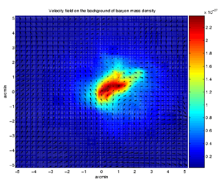
Figure 1: The velocity field is shown on the background of the baryon mass density; arrow length is linearly proportional to velocity magnitude. Color density scale is in units of $g/cm^{3}$.

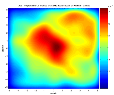
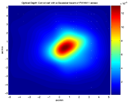
Figure 2: The gas temperature (top figure, with color scale in K) and optical depth (bottom)

The simulation was then re-initialized at $z=30$ with both dark matter and baryons ($\Omega_{b}=0.04,\,\Omega_{CDM}=0.26$) with a 128³ top grid and 2 static nested grids covering the Lagrangian volume where the cluster forms, giving an effective root grid resolution of 512³ cells (0.5 Mpc/h comoving) and dark matter particles of mass $1.49\times 10^{10}$ M_⊙. Adaptive mesh refinement is allowed in the region where the galaxy cluster forms with a total of 7 levels of refinement beyond the root grid, for a maximum spatial resolution of 15.625 h^-1 kpc (comoving). This simulation was then evolved to $z=0.06$, following the evolution of the dark matter and using adiabatic gas dynamics. The galaxy cluster of interest was then relocated with the Hop algorithm at $z=0.06$, $0.25$, $0.5$ and $1.0$, and data cubes with 256³ cells containing $\rho_{DM}$, $\rho_{gas}$, $T_{e}$ and the three baryon velocity components were extracted at these redshifts. The total cube length is 4 Mpc/h, corresponding to a spatial resolution of 15.625 kpc/h (comoving). Unless otherwise noted, the results in the following sections are for the full 256³ data cubes, and are based on the simulated cluster at $z=0.5$. The baryon density and velocity field are shown in Figure 1 and the cluster projected temperature and optical depth are depicted in Figure 2.

3 CLUSTER POLARIZATION COMPONENTS

The main process that polarizes the CMB in clusters is Compton scattering of the radiation by IC electrons. Polarization levels depend on the cluster optical depth to Compton scattering, and either on the cluster velocity or gas temperature. These are typically in the $10-100$ nK range, but may reach values as high as $\sim\mu$K. We describe the main polarization components, and illustrate their predicted patterns in our fiducial cluster. As we have noted, the CMB can be polarized by Compton scattering if the radiation multipole expansion has a finite quadrupole component in the electron rest frame. This can be brought about in several ways, as described in the following subsections. The level of linear polarization and its orientation are determined by the two Stokes parameters

$$Q = \frac{3\sigma_{T}}{16\pi}\int n_{e}dl\int\sin^{2}\alpha\cos 2\psi I(\alpha,\psi)d\Omega$$

$$U = \frac{3\sigma_{T}}{16\pi}\int n_{e}dl\int\sin^{2}\alpha\sin 2\psi I(\alpha,\psi)d\Omega,$$ (1)

where $dl$ is a length element along the photon path, $n_{e}$ is the electron number density, $\sigma_{T}$ is the Thomson cross section, and $\alpha$ and $\psi$ define the relative directions of the incoming and outgoing photons. The average electric field describes the polarization plane with a direction given by

$$\varphi=\frac{1}{2}\tan^{-1}\frac{U}{Q}.$$ (2)

When the incident radiation is expanded in spherical harmonics

$$I(\alpha,\psi)=\sum_{l,m}I_{lm}Y_{lm}(\alpha,\psi),$$ (3)

it becomes evident (from the orthogonality conditions of the spherical harmonics) that only the quadrupole moment terms proportional to $I_{2,2}$ and $I_{2,-2}$ contribute to $Q$ and $U$ in Equation (1).

In the following subsections we describe the polarization produced by Compton scattering when a quadrupole moment is induced by electron motions. These ‘kinematic’ polarization components arise due to either bulk (peculiar) or thermal (random) motion of the electrons. Since we are mainly interested in a more realistic assessment of the various components based on the results of hydrodynamic simulation (rather than idealized analytic models), previously derived theoretical expressions are only briefly summarized here.

3.1 POLARIZATION INDUCED BY THE GLOBAL CMB QUADRUPOLE

The CMB global quadrupole moment originates in the Sachs-Wolfe (SW) effect at the surface of last scattering, and later in the evolving gravitational fields of density inhomogeneities - the integrated Sachs-Wolfe (ISW) effect. Scattering by IC electrons polarizes the radiation at a level that is (linearly) proportional to the rms of the primary quadrupole moment and the cluster optical depth to Compton scattering, $\tau$ (Sazonov & Sunyaev 1999). Using the WMAP normalization of the CMB quadrupole moment (Bennett  et al.  2003) the maximal polarized signal is expected to be $\simeq 2.6\tau\,\mu K$, and its all-sky average is $\sim 60\%$ of this value (Sazonov & Sunyaev 1999). The polarization pattern has broad peaks extending over an appreciable fraction of the sky. The minima are narrow and correspond to the change of sign of the Stokes parameters. It has been noted that the dependence of this polarization component on the CMB quadrupole moment could possibly be exploited as a means to reduce cosmic variance (Kamionkowski & Loeb 1997), and as a probe of dark energy models through the redshift evolution of the quadrupole (see, however, Portsmouth 2004). We note that the polarization due to the CMB quadrupole can be distinguished from the other cluster polarization components by virtue of its large-scale distribution reflecting that of the primary CMB quadrupole (e.g. Baumann & Cooray 2003), and the fact that it is independent of frequency (when expressed in temperature units). This polarization component, which was recently studied in the context of N-body simulations by Amblard & White (2004), will not be discussed further here.

3.2 POLARIZATION DUE TO INTRINSIC QUADRUPOLE MOMENTS

Scattering of the CMB in a cluster results in local anisotropy due to the different pathlengths of photons arriving from various directions to a given point. The optical depth effectively develops a dipole moment, and $\Delta T/T$ would appear anisotropic, except in the center of a spherically symmetric cluster, where electrons effectively ’see’ almost isotropic (singly) scattered radiation. The local anisotropy of $\Delta T/T$ resulting from single scatterings is due to either thermal or bulk electron motions, constituting the well known thermal and kinematic components of the S-Z effect. This anisotropy provides the requisite quadrupole moment; second scatterings then polarize the radiation.

Two polarization components are directly induced by scattering in a moving cluster. The first is linear in the cluster velocity component transverse to the los, $v_{t}\equiv c\beta_{t}$, but quadratic in $\tau$; the second is linear in $\tau$ but quadratic in $\beta_{t}$. A third polarization component arises from second scatterings (and, therefore, is $\propto\tau^{2}$) after local anisotropy is produced by the thermal S-Z effect. The spatial patterns of the various polarization components can be readily determined only when the morphology of the cluster and its IC gas are isotropic. The polarization patterns arising from scattering off thermal electrons are isotropic (Sazonov & Sunyaev 1999) in a spherical cluster, while the corresponding patterns of the kinematic components are clearly anisotropic due to the asymmetry introduced by the direction of the cluster motion.

To calculate the polarization components, we first note that the expressions for the $Q$ and $U$ Stokes parameters are specified in Equation (1) in terms of the relative directions of the ingoing and outgoing photons. Due to the obvious dependence of the angles and frequencies on the relative directions of the electron and photon motions, the expressions for $Q$ and $U$ are transformed to a frame whose $Z$ axis coincides with the direction of the electron velocity, the axis with respect to which the incoming and outgoing photon directions are defined (in accord with the choice made by Chandrasekhar 1950). Since the Doppler effect depends only on the angle between the photon wave vector and the electron velocity, the calculation of the temperature anisotropy and polarization is easier if we assume the incident radiation is isotropic in the CMB frame (which is indeed the case to the level of accuracy relevant to this work). With the polarized cross section for Compton scattering (in the Thomson limit) written in terms of angles measured with respect to the electron velocity (after averaging over the azimuthal angles),

$$\frac{d\sigma}{d\Omega}=\frac{3\sigma_{T}}{8}\left(1-\mu_{0}^{2}\right)P_{2}(\mu^{\prime}_{0})\,,$$ (4)

where $P_{2}(\mu^{\prime}_{0})$ is the second Legendre polynomial, the expression for the $Q$ parameter of the scattered radiation is

$$Q(\mu)=\frac{3}{8}\tau(1-\mu_{0}^{2})\int_{-1}^{1}P_{2}(\mu^{\prime}_{0})I(\mu^{\prime}_{0})d\mu^{\prime}_{0}\,.$$ (5)

Here, $\mu^{\prime}_{0}=\cos\theta^{\prime}_{0}$, $\mu_{0}=\cos\theta_{0}$, are the angle cosines between the electron velocity and the incoming and outgoing photons, respectively.

3.2.1 The $\tau^{2}\beta_{t}$ and $\tau\beta_{t}^{2}$ Components

The degree of polarization induced by the kinematic S-Z component was determined by Sunyaev & Zeldovich (1980) in the simple case of uniform gas density,

$$Q=\frac{1}{40}\frac{xe^{x}}{e^{x}-1}\tau^{2}\beta_{t},$$ (6)

where $x=h\nu/kT$ is the photon dimensionless frequency, with $T$ denoting the incident CMB temperature. A more complete calculation of this and the other polarization components was formulated by Sazonov & Sunyaev (1999). Viewed along a direction $\hat{n}=(\theta,\phi)$, the temperature anisotropy at a point $(X,Y,Z)$, $\Delta T(X,Y,Z,\theta,\phi)$, generates polarization upon second scatterings. The Stokes parameters are calculated from Equation (1),

$$Q(X,Y) = \frac{3\sigma_{T}}{16\pi I_{0}}\int dZn_{e}(X,Y,Z)$$

$$\times\int d\Omega\sin^{2}(\theta)\cos(2\phi)\Delta I(X,Y,Z,\theta,\phi)$$

$$U(X,Y) = \frac{3\sigma_{T}}{16\pi I_{0}}\int dZn_{e}(X,Y,Z)$$ (7)

$$\times\int d\Omega\sin^{2}(\theta)\sin(2\phi)\Delta I(X,Y,Z,\theta,\phi)$$

where now the $Z$ direction is chosen along the los, and $I_{0}$ is the incident intensity. The intensity change resulting from first scatterings is

$$\Delta I(X,Y,Z,\theta,\phi)/I_{0}=\sigma_{T}\int d\vec{l}(X^{\prime},Y^{\prime},Z^{\prime},\theta,\phi)$$

$$\times n_{e}(X^{\prime},Y^{\prime},Z^{\prime},\theta,\phi)\hat{n}\cdot\beta(X^{\prime},Y^{\prime},Z^{\prime})$$

$$\times\frac{xe^{x}}{e^{x}-1},$$ (8)

and the optical depth thru the point $(X,Y,Z)$ in the direction $(\theta,\phi)$ is

$$\tau(X,Y,Z,\theta,\phi)=\sigma_{T}\int n_{e}(X^{\prime},Y^{\prime},Z^{\prime})d\vec{l}(X^{\prime},Y^{\prime},Z^{\prime},\theta,\phi).$$ (9)

$Q(X,Y)$ and $U(X,Y)$ fully describe the 2-D polarization field.

The second kinematic polarization component is $\propto\tau\beta_{t}^{2}$; this component is generated by virtue of the fact that the radiation appears anisotropic in the electron frame. Expanding the apparent angular distribution of the radiation in Legendre polynomials, and keeping terms up to $\beta^{2}$, the quadrupole moment is determined. The polarization of the singly scattered radiation is then calculated (Sazonov & Sunyaev 1999) by using Equation (5). (Note that the transformation back to the CMB frame does not change the polarization since this introduces additional terms which are higher order in $\beta$.) The level of this polarization component (which was originally determined by Sunyaev & Zeldovich 1980) is

$$Q=\frac{x^{2}e^{x}(e^{x}+1)}{20(e^{x}-1)^{2}}\tau\beta_{t}^{2}.$$ (10)

In our chosen frame of reference the Stokes parameter $U$ vanishes due to azimuthal symmetry, so the total polarization amplitude, $P$, is equal to $Q$ and the polarization is orthogonal to $\beta_{t}$. Relativistic corrections (to the non-relativistic expression of Sunyaev & Zeldovich 1980) were calculated by Challinor, Ford & Lasenby (2000) and Itoh et al. (2000). These corrections generally amount to a $\sim 10\%$ reduction in Q. In our calculations we use their analytic approximation (to the exact relativistic calculation)

$$Q = \frac{x^{2}e^{x}(e^{x}+1)}{10(e^{x}-1)^{2}}\tau\beta_{t}^{2}$$ (11)

$$\times\left[\frac{1}{2}F+\Theta\left(3F-2\left(2F^{2}+G^{2}\right)+\frac{1}{2}F\left(F^{2}+2G^{2}\right)\right)\right.$$

$$+ \left.\beta_{r}\left(-\frac{1}{2}F+\frac{1}{4}\left(2F^{2}+G^{2}\right)\right)\right]$$

where $F=x\coth\frac{x}{2}$, $G=x/\sinh\frac{x}{2}$, $\Theta$ is the gas dimensionless temperature, and $c\beta_{r}$ is the radial component of the cluster velocity.

3.3 POLARIZATION DUE TO SCATTERING BY THERMAL ELECTRONS

Analogously to the $\tau^{2}\beta$ component discussed above, double scattering off electrons moving with random thermal velocities can induce polarization whose level is proportional to $\tau^{2}\Theta$. The anisotropy introduced by single scatterings is the usual thermal component of the S-Z effect with intensity change $\Delta I_{t}$. We use an analytic approximation to the exact relativistic calculation for $\Delta I_{t}$ that was obtained by Itoh, Kohyama & Nozawa (1998), and Shimon & Rephaeli (2004). Using the expression for $\Delta I_{t}$ (from the latter paper) in Equation (7), the polarization can be calculated as discussed above

$$\Delta I_{t}(X,Y,Z,\theta,\phi)=\frac{\sigma_{T}I_{0}x^{3}}{e^{x}-1}\sum_{i=1}^{5}f_{i}(x)\int n_{e}({\bf r})\Theta({\bf r})^{i}dl.$$ (12)

In Equation (12) the integration is along the photon path prior to the second scattering, $f_{i}(x)$ are spectral functions of $x$ that are specified by Shimon & Rephaeli (2004).

4 RESULTS

We have calculated the polarization patterns of the kinematic and thermal components using a simulation of a massive cluster at $z=0.50$, with $M_{cl}=1.4\times 10^{15}\,M_{\odot}$ and velocity dispersion of $\approx 1000$ km/s. The baryon density and the velocity field in the relevant region of the simulated cluster are shown in Figure 1. Polarization levels in all the figures are specified in terms of the equivalent (absolute) temperature. The figures show results in the sky plane with the los along the Z-axis.

The calculations of the double scattering components (proportional to $\tau^{2}\Theta$ and $\tau^{2}\beta$) are more challenging than that of the single scattering case. The calculations generally require ray tracing of doubly scattered photons. In Cartesian coordinates, Equations (7) & (12) can be written as

$$Q(X,Y) = \frac{3\sigma_{T}^{2}}{16\pi}\int\int dZd^{3}{\bf r^{\prime}}n_{e}({\bf r})n_{e}({\bf r^{\prime}})$$

$$\times\frac{(X-X^{\prime})^{2}-(Y-Y^{\prime})^{2}}{|{\bf r^{\prime}}-{\bf r}|^{4}}\sum_{i=1}^{5}f_{i}(x)\Theta({\bf r^{\prime}})^{i}$$

$$U(X,Y) = \frac{3\sigma_{T}^{2}}{8\pi}\int\int dZd^{3}{\bf r^{\prime}}n_{e}({\bf r})n_{e}({\bf r^{\prime}})$$ (13)

$$\times\frac{(X-X^{\prime})(Y-Y^{\prime})}{|{\bf r^{\prime}}-{\bf r}|^{4}}\sum_{i=1}^{5}f_{i}(x)\Theta({\bf r^{\prime}})^{i}$$

where the first integration (over $Z$) is along the los. The electron density $n_{e}$ was calculated from the simulated $\rho_{g}$ taking a molecular weight of $\mu=0.63$.

Calculation of these 4-D integrals over the simulation $256^{3}$ data cells is computationally intensive, motivating an attempt to reduce the level of computation. For example, an approximation (employed by Lavaux et al. 2004) is to describe the first scattering by representing the gas in terms of a best-fit $\beta$ - profile. This significantly reduces the extent of the calculation. From Figures 1 & 2, it is evident that our cluster cannot be fitted by a $\beta$ profile, isothermal or not; fitting merging clusters with subclumps and rich substructure with a $\beta$ profile is clearly inappropriate. Fortunately, Equation (13) can be cast in the form

$$P_{+,\times}(X,Y)=\sigma_{T}^{2}\int dZn_{e}({\bf r})h_{+,\times}({\bf r})$$ (14)

where $P_{+}$ and $P_{\times}$ are the Stokes $Q$ & $U$ parameters, respectively, and

$$h_{+,\times}=f_{+,\times}\star g$$ (15)

is a convolution of the functions $f_{+,\times}$ with $g$, where

$$f_{+} = \frac{X^{2}-Y^{2}}{r^{4}},\qquad\qquad f_{\times}=\frac{2XY}{r^{4}},\,\,$$

$$g = \sum_{i}n_{e}({\bf r})f_{i}(x)\Theta({\bf r})^{i}.$$ (16)

This representation enables us to employ 3-D FFT calculations that are considerably faster than the direct integrations of Equations (13). However, the full computation is still quite extensive; we therefore focus here on the core of the simulation volume.

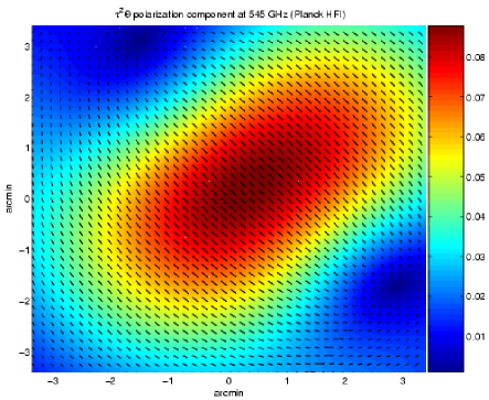
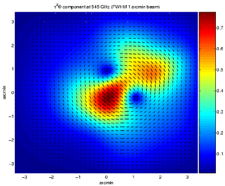
Figure 3: The $\tau^{2}\Theta$ polarization component convolved with the Planck HFI beam (top) and with a FWHM 1’ beam (bottom). Color scale is in $\mu$K.

Our results are summarized in Figure 3. Unlike the case of spherical (Sazonov & Sunyaev 1999) or quasi-spherical (Lavaux et al. 2004) clusters, we obtain a more intricate polarization pattern and the quadrupole structure, which is absent in the spherically symmetric case, is evident. This pattern reflects the non-uniform gas distribution and an appreciable degree of non-sphericity of the cluster, which substantially affect primarily the double scattering polarization signals, essentially due to the fact that the second scattering is more likely to occur far from the cluster center (see also Sazonov & Sunyaev 1999, Lavaux  et al.  2004). The level of polarization at the 545 GHz Planck frequency band, at which the beam is 4.5’ FWHM, can reach $\sim 80$ nK, but when convolved with a narrow beam 1’ FWHM profile, its peak value can be as high as $\sim 0.7\mu K$. This level definitely grazes the threshold of next generation experiments. Note, however, that we have considered a rich cluster with maximal optical depth of $\tau_{0}\approx 0.01$ (Figure 2), but since this component is proportional to $\sim\tau^{2}$, typical values could be a factor $\sim 4$ lower or higher than the specific values quoted here. Additional uncertainty stems from the scaling of the cluster temperature with mass, and from the evolution of the temperature with redshift. Finally, this component was calculated at 545 GHz; measurements at lower frequencies will result in lower levels of polarization (Equation 13).

Equations (7)-(9) for the double scattering kinematic component ($\propto\tau^{2}\beta$) can be written in the same form as Equation (14) , but with

$$h_{+,\times}=f_{+,\times}\star g\equiv\sum_{i=1}^{3}f_{i_{+,\times}}\star g_{i}$$ (17)

where

$$f_{i+}=\frac{X_{i}(X^{2}-Y^{2})}{r^{5}},\,\,\,f_{i\times}=\frac{2X_{i}XY}{r^{5}},\,\,\,g_{i}=n({\bf r})\beta_{i}({\bf r})$$ (18)

with $X_{i}$ ($i=1,2,3$) the components of the vector $(X,Y,Z)$. The results for the $\tau^{2}\beta$ component (for the central region of the simulation) are summarized in Figure 4. The level of polarization in absolute temperature units is $\sim 1-2$ orders of magnitudes smaller than the $\propto\tau^{2}\Theta$ component. Convolving with the Planck HFI and a gaussian beam profile with FWHM of 1’, the peak values are $3$ nK and $25$nK, respectively, comparable to the level of the cosmological quadrupole polarization (section 3.1). As previously noted, both these components are frequency-independent, a fact that has obvious implications on the feasibility of separating these components out when the measurements will eventually reach the requisite sensitivity.

The polarization at 545 GHz due to the Doppler anisotropy, $\propto\tau\beta^{2}$, is plotted in Figure 5. At this high frequency the polarization can be as high as $\sim 18$ nK when convolved with the Planck HFI. Convolution with a narrow gaussian with 1’ FWHM beam yields higher ($\sim 0.1\mu K$) levels. Owing to its spectral dependence, this component can - in principle - be distinguished from both the $\propto\tau^{2}\Theta$ and $\propto\tau^{2}\beta$ polarization by multi-frequency measurements. Moreover, due to the different dependence on the optical depth, the two kinematic effects ($\propto\tau^{2}\beta$ and $\propto\tau\beta^{2}$) can possibly be separated out through their different morphologies (compare Figures 4 & 5).

5 DISCUSSION

CMB observational capabilities have dramatically improved since the first measurement of the primary anisotropy by COBE/DMR. With projected sensitivities around $1$ $\mu$K, and sub-arcminute angular resolution, measurement of the dominant polarization signals in clusters by upcoming experiments seems feasible in the (not too distant) future.

The coupling of the CMB to IC gas by Compton scattering leads to various polarization components whose magnitudes and spatial patterns could provide significant information on the cluster motion and the dynamical state of IC gas. The feasibility of identifying a given polarization component (obviously) depends primarily on its magnitude, but this will be aided also by its particular spectral and spatial characteristics. The fact that some of the spatial patterns (such as that of the thermal S-Z polarization) produce no net signal (or substantially reduced signal in aspherical cluster) when integrated over a sufficiently large region of the cluster surface, can be exploited in optimizing the observational strategy for measurement of a specific polarization component.

In this work we have used cluster simulations to assess the amplitude of three CMB polarization components. As expected, most polarization signals induced by the interaction of CMB photons and IC gas are substantially smaller than $1\,\mu$K. An exception is the polarization induced by the double scattering thermal effect. For this component, convolving our simulation data with a FWHM 1’ beam, we find that the effective polarization signal is about $\sim 1\mu K$. The polarization induced by double scattering off the thermal gas was the focus of the work by Lavaux  et al.  (2004). We have implemented a direct calculation scheme that yields results at the cluster core which qualitatively differ from those of the latter authors. By assuming isothermal $\beta$ profile to describe first scatterings, Lavaux  et al.  (2004) partially underestimated the effect of dynamics on producing the quadrupole in the first scattering; this may be a reason for the qualitative discrepancy between our respective results. By exploiting the properties of convolution integrals we are able to considerably facilitate the calculation of the components $\propto\tau^{2}\Theta$, $\propto\tau^{2}\beta$, essentially avoiding the need for simplifying approximations. The $\propto\tau^{2}\beta$ and $\propto\tau\beta^{2}$ components are an order of magnitude weaker, too small to be detected towards individual clusters in near future experiments.

This is the first stage of a comprehensive study of CMB polarization in clusters based on a realistic description of cluster structure that is afforded by hydrodynamic simulations. The results presented here already point to appreciable discrepancy with what is obtained when IC gas is modeled by a simple spherical distribution. We plan to extend the work presented here to a sample of simulated clusters with a range of masses and redshifts. The polarization signals in each of the sampled clusters together, supplemented by the expected confusing polarized signals, will then be analyzed in order to determine optimal strategies for the measurement of cluster-induced polarization components and the extraction of cluster properties.

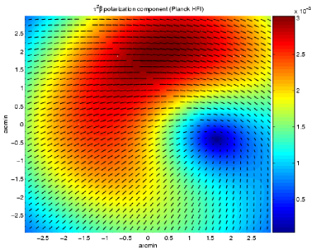
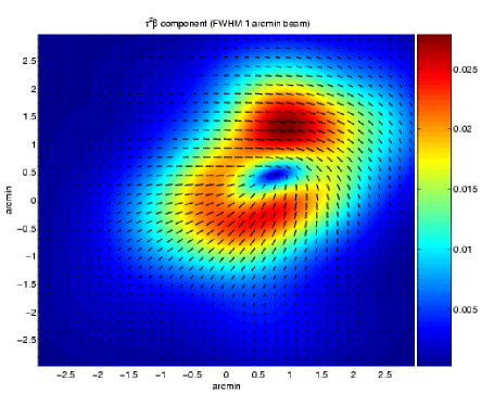
Figure 4: The $\tau^{2}\beta$ polarization component convolved with the Planck HFI beam (top) and with a FWHM 1’ beam (bottom). Color scale is in $\mu$K.

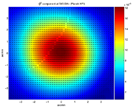
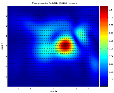
Figure 5: The $\tau\beta^{2}$ polarization component at 545 GHz convolved with the Planck HFI beam (top) and with a FWHM 1’ beam (bottom). Color scale is in $\mu$K.

References

- (1) Amblard, A. & White, M., astro-ph/0409063
- (2) Baumann, D., & Cooray, A. 2003, New Astronomy Review, 47, 839
- (3) Bennett, C., et al. 2003, ApJS, 148, 1
- (4) Berger, M.J. & Colella, P. 1989 J. Comput. Phys, 82, 64
- (5) Birkinshaw, M. 1999, Physrep, 310, 97
- (6) Bowden, M., et al. 2004, MNRAS, 349, 321
- (7) Bryan, G.L., Norman, M.L., Stone, J.M., Cen, R., & Ostriker, J.P. 1995, Compute. Phys. Commun, 89, 149
- (8) Carlstrom, J. E., Holder, G. P., & Reese, E. D. 2002, ARA & A, 40, 643
- (9) Challinor, A. D., Ford, M. T., & Lasenby, A. N. 2000, MNRAS, 312, 159
- (10) Chandrasekhar, S. 1950, Oxford, Clarendon Press, 1950
- (11) Cooray, A., Melchiorri, A., Silk J. astro – ph/0205214
- (12) Eisenstein, D.J. & Hut, P. 1998 ApJ, 498, 137
- (13) Gibilisco, M. 1997, Ap & SS, 249, 189
- (14) Kamionkowski, M. & Loeb, A. 1997, PRD, 56, 4511
- (15) Itoh, N., Kohyama, Y., & Nozawa, S. 1998, ApJ, 502, 7
- (16) Itoh, N., Nozawa, S., & Kohyama, Y. 2000, ApJ, 533, 588
- (17) Lavaux, G., Diego, J. M., Mathis, H., & Silk, J. 2004, MNRAS, 347, 729
- (18) Ohno, H., Takada, M., Dolag, K., Bartelmann, M., & Sugiyama, N. 2003, ApJ, 584, 599
- (19) O’Shea, B.W., Bryan, G., Bordner, J., Norman, Michael L., Abel, T., Harknes, R. and Kritsuk, A. 2004. In “Adaptive Mesh Refinement - Theory and Applications”, Eds. T. Plewa, T. Linde & V. G. Weirs, Springer Lecture Notes in Computational Science and Engineering, 341
- (20) Portsmouth, J. 2004, PRD, 70, 063504
- (21) Rephaeli Y., 1995, ARA& A. 33, 541
- (22) Sazonov, S. Y. & Sunyaev, R. A. 1999, MNRAS, 310, 765
- (23) Shimon, M., & Rephaeli, Y. 2004, New Astronomy, 9, 69
- (24) Sunyaev, R. A. & Zeldovich, I. B. 1980, MNRAS, 190, 413
- (25) Woodward, P.R. & Colella, P. 1984 J. Comput. Phys., 54, 115