On the incidence rate of first overtone Blazhko stars in the Large Magellanic Cloud

Abstract

Aims. By using the full span of multicolor data on a representative sample of first overtone RR Lyrae stars in the Large Magellanic Cloud (LMC) we revisit the problem of the incidence rate of the amplitude/phase-modulated (Blazhko) stars.

Methods. Multicolor data, obtained by the MAssive Compact Halo Objects (MACHO) project, are utilized through a periodogram averaging method.

Results. The method of analysis enabled us to increase the number of detected multiperiodic variables by $18$% relative to the number obtained by the analysis of the best single color data. We also test the maximum modulation period detectable in the present dataset. We find that variables showing amplitude/phase modulations with periods close to the total time span can still be clearly separated from the class of stars showing period changes. This larger limit on the modulation period, the more efficient data analysis and the longer time span lead to a substantial increase in the incidence rate of the Blazhko stars in comparison with earlier results. We find altogether 99 first overtone Blazhko stars in the full sample of 1332 stars, implying an incidence rate of $7.5$%. Although this rate is nearly twice of the one derived earlier, it is still significantly lower than that of the fundamental mode stars in the LMC. The by-products of the analysis (e.g., star-by-star comments, distribution functions of various quantities) are also presented.

1 Introduction

Current analyses of the databases of the microlensing projects MACHO and OGLE (Optical Gravitational Lensing Experiment) have led to a substantial increase in our knowledge on the frequency of the amplitude/phase-modulated RR Lyrae (Blazhko [BL] ) stars. Moskalik & Poretti (2003) analyzed the OGLE-I data on 215 RR Lyrae stars in the Galactic Bulge. They found incidence rates for the fundamental (RR0) and first overtone (RR1) Blazhko stars of $23$% and $5$%, respectively. A similar analysis by Mizerski (2003) on a much larger dataset from the OGLE-II database yielded $20$% and $7$%, respectively. These rates, at least for the RR0 stars, are very similar to the ones suggested some time ago by Szeidl (1988) from the various past analyses of rather limited data on Galactic field and globular cluster stars. One gets smaller rates by analyzing the RR Lyrae stars in the Magellanic Clouds. Based on the OGLE-II observations of a sample of 514 stars in the Small Magellanic Cloud (SMC), in a preliminary study, Soszyński et al. (2002) obtained the same rate of $10$% both for the RR0 and RR1 stars. In a similar study on a very large sample containing 7110 RR Lyrae stars in the LMC, Soszyński et al. (2003) derived $15$% and $6$% for the RR0 and RR1 stars, respectively. In earlier studies on the same galaxy, based on the observations of the MACHO project, Alcock et al. (2000, 2003, hereafter A00 and A03, respectively) got rates of $12$% and $4$% for the above two classes of variables. One may attempt to relate these incidence rates to the metallicities of the various populations (e.g., Moskalik & Poretti 2003), but the relation (if it exists) is certainly not a simple one (Kovács 2005; Smolec 2005).

Except for the SMC, all investigations indicate much lower incidence rates for RR1$-$BL stars than for RR0$-$BL ones. It is believed that the cause of this difference is internal, i.e., due to real difference in physics and can not be fully accounted for by the possibly smaller modulation amplitudes of the RR1 stars. Since this observation may have important consequences on any future modeling of the BL phenomenon, we decided to re-analyze the MACHO database and utilize all available observations (i.e., full time span two color data). In Sect. 2 we summarize the basic parameters of the datasets and some details of the analysis. Section 3 describes our method for frequency spectrum averaging. The important question of the longest detectable BL period from the present dataset and the concomitant problem of variable classification are dealt with in Sect. 4. Analysis of the RR1 stars with their resulting classifications will be presented in Sect. 5. Finally, in Sect. 6 we summarize our main results with a brief discussion of the current state of the field.

2 Data, method of analysis

For comparative purpose, in the first part of our analysis, we use the same dataset as the one employed by A00. Our final results are based on the full dataset spanning $\sim 7.5$ years. Basic properties of these two sets are listed in Table 1. Both sets contain the same $1354$ stars and cover the fields # 2, 3, 5, 6, 9, 10, 11, 12, 13, 14, 15, 18, 19, 47, 80, 81 and 82, sampling basically the LMC bar region. Because the selection of the stars was made earlier on simple preliminary criteria such as period and color, some variables, other than first overtone RR Lyrae stars, were also included. Fortunately, the number of these other variables is only 22, that is small relative to the full sample.

Table 1: Properties of the LMC RR1 datasets analyzed in this paper

Set	$\langle T_{\rm tot}\rangle$	$\langle N_{\rm d}\rangle$	Colors
#1	$6.5$	$700$	‘r’, ‘b’
#2	$7.5$	$900$	‘r’, ‘b’

Notes: $\langle T_{\rm tot}\rangle=$ average total time span [yr]; $\langle N_{\rm d}\rangle=$ average number of datapoints per variable; Colors: MACHO instrumental magnitudes, see Alcock et al. (1999)

We employed a standard Discrete Fourier Transform method by following the implementation of Kurtz (1985). All analyses were performed in the $[0,6]$ d^-1 band with $150000$ frequency steps, ensuring an ample sampling of the spectrum line profiles even for the longest time series. The search for the secondary frequencies was conducted through successive prewhitenings in the time domain. The first step of it consisted of the subtraction of the main pulsation component together with its harmonics up to order three. In all cases the frequency of the given component was made more accurate by direct least squares minimization. When the two colors were used simultaneously, we allowed different amplitudes and phases for the two colors and minimized the harmonic mean of the standard deviations of the respective residuals. Although somewhat arbitrarily, we considered the harmonic mean as a useful function for taking into account differences in the data quality.

For the characterization of the signal-to-noise ratio (SNR) of the frequency spectra we use the following expression

$${\rm SNR}={A_{\rm p}-\langle A_{\nu}\rangle\over\sigma_{A_{\nu}}}\hskip 5.69054pt,$$ (1)

where $A_{\rm p}$ is the amplitude at the highest peak in the spectrum, $\langle A_{\nu}\rangle$ is the average of the spectrum and $\sigma_{A_{\nu}}$ is its standard deviation, computed by an iterative $4\sigma$ clipping.

3 Spectrum Averaging Method (SAM)

Unlike OGLE, where measurements are taken mostly in the $I_{c}$ band (e.g., Udalski, Szymański & Kubiak, M. 1997), the MACHO database has roughly equal number of measurements in two different colors for the overwhelming majority of the objects (e.g., Alcock et al. 1999). This property of the MACHO database enables us to devise a method that uses both colors for increasing the signal detection probability.

It is clear that simple averaging of the time series of the different color bands cannot work, because: (a) the two time series are systematically different due to the difference in colors; (b) sampling may be different for hardware, weather or other reasons. Therefore, we are resorted to some spectrum averaging method that uses the frequency spectra of the two time series rather than their directly measured values. Obviously, SAM is also affected by the time series properties mentioned above. However, this effect is a weaker, because: (i) we are interested in the positions of the peaks in the spectra and these are the same whatever colors are used; (ii) spectral windows are similar, unless the samplings of the two time series are drastically different. As an example for the fulfilment of this latter condition for the MACHO data, in Fig. 1 we show the spectral windows in the two colors in one representative case.

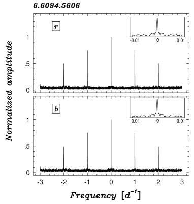
Figure 1: Example of the similarity of the spectral windows of the MACHO instrumental ‘r’ and ‘b’ time series. Close-ups of the main peaks are displayed in the insets. The MACHO identification number of the star analyzed is shown in the upper left corner of the figure.

In order to optimize noise suppressing, we compute the summed spectrum by weighting the individual spectra by the inverse of their variances

$$S_{i}={\sigma_{\rm r}^{2}\sigma_{\rm b}^{2}\over\sigma_{\rm r}^{2}+\sigma_{\rm b}^{2}}\Bigl{(}{1\over\sigma_{\rm r}^{2}}R_{i}+{1\over\sigma_{\rm b}^{2}}B_{i}\Bigr{)}\hskip 5.69054pt,$$ (2)

where $R_{i}$ and $B_{i}$ are the amplitude spectra of the ‘r’ and ‘b’ data, $\sigma_{\rm r}$ and $\sigma_{\rm b}$ are the standard deviations of the spectra.

Before we discuss the signal detection capability of SAM, it is necessary to give significance levels for periodic signal detection when using the present dataset. Perhaps the simplest way of doing this is to perform a large number of numerical simulations and derive an empirical distribution function of SNR. For this goal we generated pure Gaussian noise on the observed time base of 10 randomly selected stars. For each object we generated 1000 different realizations and computed the frequency spectra in our standard frequency band of $[0,6]$ d^-1. The empirical distribution function was derived from the 10000 SNR values computed on these spectra. Figure 2 shows the resulting functions for the single color and SAM spectra. For further reference, the 1% significance levels are at $6.9$ and $6.5$ for the single color and SAM spectra, respectively. All signals that have lower SNR values than these, are considered to be not detected in the given time series. The lower cutoff for the SAM spectra is the result of the averaging of independent spectra which also results in a greater number of independent points in the SAM spectra and concomitantly, in a slightly different shape of the distribution functions (see also Kovács, Zucker & Mazeh 2002).

Figure 2: Probability distribution functions of SNRs of the amplitude spectra of pure Gaussian noise generated on the time base of the ‘r’ data (dotted line), ‘b’ data (dashed line) and their combination by SAM (solid line).

In turning to the signal detection efficiency of SAM, we note the following. At very low SNR we expect no improvement by applying SAM, because the optimally achievable noise suppression is insufficient for the signal to emerge from the noise. In the other extreme, when the the signal is strong, the improvement is expected to be minimal and secure detection is possible without employing SAM. In order to verify this scenario, we conducted tests with artificial data. The result of one of these tests is shown in Fig. 3. The test data were generated on the 7.5 year time base given by the variable 10.3434.936. The signal consisted of a simple sinusoidal with a period of $0.278$ d and amplitude $A$, where $A$ was chosen to be the same in both colors and changed in $100$ steps between $0.01$ and $0.3$ to scan different SNR values. At each value of the amplitude we added Gaussian noise of $\sigma=0.11$ to the signal. This procedure was repeated for $100$ different realizations. At each color and amplitude we computed the average and standard deviation of the SNR values obtained from these $100$ realizations. In order to characterize the gain by employing SAM, we also computed the ratio of the SNR values ($R_{\rm SNR}$) as derived from the single color data and by the application of SAM.

Figure 3: Uppermost panel: variation of the ensemble average of $R_{\rm SNR}={\rm SNR}_{\rm SAM}/{\rm SNR}_{\rm color}$ as a function of the test amplitude. Open circles refer to the ‘r’ data, crosses to the ‘b’ data. Middle panel: close-up of the low/mid SNR region of the above diagram. Error bars show the $1\sigma$ ranges of the values obtained by the various noise realizations. Lowermost panel: ensemble average of SNR. The dots are for the SAM values. Short- and long-dashed lines show the $1$% noise probability levels at SNR $=6.9$ and SNR $=6.5$, corresponding to the single-color and SAM spectra, respectively (see also text and Fig. 2 for further details).

We see from Fig. 3 that there is a region where the signal has too low amplitude to be detected in the single color data, but not low enough to remain hidden in the SAM spectra. This is the most interesting amplitude/noise regime, where the application of SAM results in new discoveries. At higher amplitudes SAM leads ‘only’ to an increase in SNR. It is seen that the maximum increase in SNR is at around $\sqrt{2}$, as expected from elementary considerations.

In order to show non-test examples for the signal detection efficiency of SAM, in Figs. 4 and 5 we exhibit the method at work for the observed data of two variables. In both cases the single color data are insufficient for detection, but the combined spectra show clearly the presence of the signal.

Figure 4: Example of the signal detection efficiency of SAM at low SNR level, when the single color data do not show the presence of the signal. Upper and middle panels show the frequency spectra for the ‘r’ and ‘b’ data, whereas the lower one exhibits the SAM result. The MACHO star identification number is shown at the top, whereas the SNR values are given in the corresponding panels. All spectra are displayed in the same (arbitrary) scale.

Figure 5: As in Fig. 4, but for the case when the signal is at the verge of detection in the single color data and SAM increases the reliability of the detection.

By analyzing all the 1354 variables of set #1 we can count the number of cases when significant components are found after the first prewhitening. The result of this exercise is shown in Table 2. We see that there is a strong support of the obvious assumption that application of two color data significantly increases the detection probability of faint signals. The gain is 18% relative to the best single color detection rate.

Table 2: Number of single- and multi-periodic variables in set #1 of Table 1.

Color	r	b	SAM
$N_{1}$	$978$	$895$	$813$
$N_{2}$	$376$	$459$	$541$
$N_{2}/(N_{1}+N_{2})$	$27.8$%	$33.9$%	$40.0$%

Notes: $N_{1}=$ number of single-periodic variables; $N_{2}=$ number of multi-periodic variables

4 The phenomenological definition of the BL stars – Separation of the BL and PC variables

The current loose definition of the BL stars relies purely on the type of the frequency spectra of their light or radial velocity variations. Usually those RR Lyrae stars are called BL variables that exhibit closely spaced peaks in their frequency spectra. Although most of the variables classified as type BL contain only one or two symmetrically spaced peaks at the main pulsation component, complications arise when, after additional prewhitenings, significant components remain, or, when the prewhitening is ambiguous, due to the closeness of the secondary components. There are two basic cases of complication: (i) the remnant components are not well-separated and few successive prewhitenings do not lead to a complete elimination of the secondary components; (ii) we have several well-defined additional peaks, whose pattern is different from the ones usually associated with the BL phenomenon (single-sided for BL1 and symmetrically spaced for BL2 patterns).

Case (i) can be considered as a consequence of some non-stationarity in the data, leading to a nearly continuous spectral representation, whereas case (ii) can be related perhaps to some modulation of more complicated type than that of the BL phenomenon. In order to make the phenomenological classification of variable types as clear as possible, supported by the test to be presented below, we adopt the following definitions:

• • (period changing stars): Close components (i.e., the ones that are close to the main pulsation frequency) cannot be eliminated within three prewhitenening cycles, or, if they can, their separation from the main pulsation component is less than $\sim 1/T$, where $T$ is the total time span. Furthermore, except for possible harmonics, there are no other significant components in the spectra.

• • (Blazhko stars): There is either only one or two symmetrically spaced close components on both sides of the main pulsation frequency. After the second or third prewhitenings, except for possible harmonics, no significant pattern remains or the pattern is of type PC.

• • (stars with closely spaced multiple frequency components): All close components are well-separated (i.e., frequency distances are greater than $\sim 1/T$) and, except if there are only two secondary components on one side of the main pulsation frequency, more than three prewhitenings are necessary to eliminate all of them.

We note that possible appearance of instrumental effects (i.e., peaks at integer d^-1 frequencies) is disregarded in the above classification. Class MC is equivalent to class $\nu$M used in A00 and A03. Here the new notation is merely aimed at simplification on the occasion of the above definition. Furthermore, in the previous works, variables with “dominantly” BL2 structures were included in class BL2. Now the above scheme puts them among the MC stars.

Based on the following test, we note that below frequency separations less than $\sim 1.5/T$, distinction among the above types becomes more ambiguous, because in the simple prewhitening technique followed in this paper, the result will depend on the phase of the modulation.

In order to substantiate the above definitions, here we examine in more detail how we can distinguish between the PC and BL phenomena based solely on the properties of the prewhitened spectra.

We use the time distribution of arbitrarily selected stars to generate artificial time series with modulated signal parameters given in Table 3. We see that the chosen types of modulation cover nearly all basic cases in the lowest order approximation (i.e., single main pulsation component with frequency $\omega_{0}$, linear period change, etc.). No noise is added, because we are interested in differences caused by the various non-stationary components in the residual spectra, after prewhitened by the pulsation component. Nevertheless, noise plays an important role at low modulation levels, but a more detailed study of the complicated problem of non-stationary signal classification in the presence of noise is out of the scope of the present work.

Table 3: Definition of the signals used in the BL/PC variability test.

Type	Time dependence
AM	$A(t)=A\sin(\Omega t+\Phi)$; $\omega(t)$, $\varphi(t)=$ const.
PM	$\varphi(t)=A_{\varphi}\sin(\Omega t+\Psi)$; $\omega(t)$, $A(t)=$ const.
FM	$\omega(t)=\omega_{0}+A_{\omega}\sin(\Omega t+\Gamma)$; $A(t)$, $\varphi(t)=$ const.
PC	$\omega(t)=\omega_{0}/(1+\beta t/P_{0})$; $A(t)$, $\varphi(t)=$ const.

Notes: Signal form: $x(t)=(1+A(t))\sin(\omega(t)t+\varphi(t))$; $\omega_{0}=2\pi/P_{0}$; $P_{0}=0.377$; $\Omega=2\pi/P_{\rm BL}$; $P_{\rm BL}=$ BL period; AM=amplitude modulation; PM=phase modulation; FM=frequency modulation; PC=secular frequency change; $\Phi$, $\Psi$, $\Gamma$ are arbitrary constant phases.

The same pulsation period of $0.377$ d is used for 10 randomly selected stars. For each star, we scan the modulation frequency $\Omega$ and the rate of period change $\beta$ at fixed values of all the other parameters. Amplitudes are adjusted to get modulation levels that are 20% of the peak of the main pulsation component in the frequency spectra. Parameter $\beta$ is changed in the range of $(1$–$12)\times 10^{-8}$, yielding modulation levels between $20$% and $50$%. Each scan is repeated with 10 randomly selected phase values. By using the same code for the analysis of these artificial signals as the one employed for the observed data, we get the result shown in Fig. 6. In order to characterize the efficiency of the prewhitening, here we use the ratio $A_{3}/A_{1}$, where $A_{1}$ and $A_{3}$ denote the peak amplitudes after the first and third prewhitenings, respectively. Although in practice we use the SNR of the frequency spectra to select significant components, here the direct comparison of the amplitudes is more meaningful, because for noiseless signals SNR can be high even if the peak amplitude itself is small.

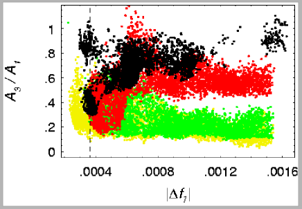
Figure 6: Testing various modulated signals as given in Table 3. The ratio of the peak amplitudes after the third and first prewhitenings are plotted as a function of the measured frequency distance (in [d^-1]) from the main pulsation component. Dashed vertical line shows the position of the $1/T$ frequency, where $T$ denotes the total time span. Dots of different shades/colors are for the various modulation types: yellow/light gray, green/gray, red/dark gray and black are for AM, PM, FM and PC, respectively. The separation of simple amplitude and phase modulations from the more complicated ones (FM and PC) are clearly visible at $|\Delta f_{1}|>2/T$.

It is clear from the figure that PC signals remain difficult to prewhiten, except perhaps near and below $1/T$, when any types of signal can be prewhitened due to the proximity to the main pulsation component. Although periodic frequency modulation behaves similarly to secular period change above $1.5/T$, it can be prewhitened (and therefore confused) with simple amplitude and phase modulations below this limit. When the secular change or periodic modulation of the pulsation frequency is strong, they are more easily separated from simple modulated signals (of types AM and PM, see Table 3). This happens at measured modulation frequencies greater than $\sim 2/T$ (see the gap starting at $\sim 0.0008$ d^-1). Additional separation between AM and PM signals is observable at modulation frequencies greater than $\sim 5/T$ , where, as expected, the AM type leaves the weakest trace after the third prewhitening.

We conclude that the standard method of prewhitening we use for the analysis of the observed data is capable of making distinction between linear period change and signal modulation, but confusion occurs with periodic frequency modulations under observed modulation frequencies of $1.5/T$. Modulation types AM and FM are also difficult to distinguish, except for short modulation periods, when type AM can be prewhitened more easily. These results support our phenomenological classification of variables given at the beginning of this section even in the case of long modulation periods.

5 New detections by using SAM

Here we re-address the question of the incidence rate of first overtone BL stars by applying the method of analysis and scheme of classification described in the previous sections.

Table 4: Final classification of the 1354 pre-selected variables

Classification	Short description	Number	Inc. rate in RR1
RR1–S	Singly-periodic overtone RR Lyrae	$712$	$53.5\,$%
RR1–BL1	RR1 with one close component	$46$	$3.5\,$%
RR1–BL2	RR1 with symmetric frequencies	$53$	$4.0\,$%
RR1–MC	RR1 with more close components	$13$	$1.0\,$%
RR1–PC	RR1 with period change	$187$	$14.0\,$%
RR1–D	RR1 with frequencies at integer $d^{-1}$	$137$	$10.3\,$%
RR1–MI	RR1 with some miscellany	$13$	$1.0\,$%
RR01	FU/FO double-mode RR Lyrae	$165$	$12.4\,$%
RR01–BL1		$1$	$0.1\,$%
RR01–PC		$5$	$0.4\,$%
RR0–S	Fundamental mode RR Lyrae	$1$	$-$
RR0–BL1		$1$	$-$
RR0–BL2		$1$	$-$
MDM	Mysterious double-mode	$3$	$-$
BI	Eclipsing binary	$16$	$-$

Table 5: Notebook of the analysis

MACHO ID	Period	Type $r$	Type $r,\,b$	Type $r,\,b$	Comments
		(A00)	(SAM)	(SAM)
	[d]	6.5 years		7.5 years
10.3190.501	0.3527946	RR1-S	RR1-S	RR1-S
10.3191.363	0.4060709	RR01	RR01	RR01
10.3193.457	0.2977060	RR1-S	RR1-S	RR1-S	weak peak in r at 0.4477
10.3193.514	0.2762716	RR1-S	RR1-S	RR1-S
10.3310.723	0.3675948	RR1-S	RR1-S	RR1-S
10.3311.612	0.3308571	RR1-S	RR1-S	RR1-S
10.3314.787	0.3575062	RR1-S	RR1-S	RR1-S
10.3314.873	0.3842321	RR1-S	RR1-S	RR1-S
10.3314.916	0.3438987	RR1-S	RR1-S	RR1-S
10.3315.758	0.2755685	RR1-S	RR1-S	RR1-S
10.3432.666	0.3418437	RR1-S	RR1-PC	RR1-PC
10.3434.825	0.2776860	RR1-S	RR1-S	RR1-S
10.3434.936	0.2769524	RR1-S	RR1-S	RR1-S
10.3435.907	0.3295068	RR1-S	RR1-S	RR1-S
10.3550.888	0.3317657	RR1-S	RR1-S	RR1-S
10.3552.745	0.2922940	RR1-BL1	RR1-BL1	RR1-BL1
10.3556.986	0.2961494	RR1-PC	RR1-PC	RR1-PC	df=0.00038
10.3557.1024	0.2947668	RR1-PC	RR1-PC	RR1-BL2	df=0.00043

Note: This table is available in its entirety at CDS (http://cdsweb.u-strasbg.fr). Additional data (positions, magnitudes, etc.) can be found at the MACHO online database (http://wwwmacho.mcmaster.ca/Data/MachoData.html).

Table 6: Properties of the MDM stars

MACHO ID	$P_{1}$	$P_{2}/P_{1}$	$V$	$V-R$
12.10202.285	0.398	0.807	18.99	0.50
12.10443.367	0.337	0.802	18.90	0.45
9.4278.179	0.327	0.805	18.69	0.29

Table 7: Data on the first overtone Blazhko stars

MACHO ID.	$P_{1}$	$f_{\rm BL}$	$A_{+}$	$A_{0}$	$A_{-}$	MACHO ID.	$P_{1}$	$f_{\rm BL}$	$A_{+}$	$A_{0}$	$A_{-}$
10.3552.745	0.2922940	0.037408	0.0666	0.1280	$-$	6.5729.958	0.2778179	0.074254	0.1045	0.1641	$-$
10.3557.1024	0.2947668	0.000426	0.1000	0.2643	0.0941	6.5730.4057	0.2763214	0.077598	0.0662	0.1249	$-$
10.4035.1095	0.3188217	0.080780	0.0496	0.2239	$-$	6.5850.1081	0.3335893	$-$0.118341	$-$	0.1617	0.0326
10.4161.1053	0.2874579	0.094288	0.0769	0.1443	$-$	6.5971.1233	0.2877179	$-$0.073476	0.0380	0.1868	0.0666
11.9471.780	0.2859825	$-$0.113512	$-$	0.2076	0.0764	6.6091.1198	0.2668322	$-$0.075389	$-$	0.1654	0.0307
13.5713.590	0.2836353	0.100165	0.0636	0.0870	$-$	6.6091.877	0.3206106	$-$0.038525	$-$	0.1046	0.0642
13.5714.442	0.3168726	0.109252	0.0547	0.1008	$-$	6.6094.5606	0.3393854	$-$0.001244	0.0593	0.2476	0.0637
13.5842.2468	0.2731424	$-$0.084060	$-$	0.2060	0.0355	6.6326.424	0.3304519	$-$0.072633	$-$	0.2353	0.0504
13.5959.584	0.3466458	0.000993	0.0286	0.2629	$-$	6.6810.616	0.2883850	$-$0.000403	0.0552	0.2113	0.0704
13.6322.342	0.2621495	0.180083	0.0385	0.1166	$-$	6.7054.713	0.4404073	$-$0.001674	0.0445	0.2110	0.0478
13.6326.2765	0.3304520	$-$0.072702	$-$	0.2387	0.0334	6.7056.836	0.4476160	0.001120	0.0317	0.1781	0.0252
13.6810.2981	0.2883863	0.000419	0.0691	0.2050	0.0659	80.6352.1495	0.3079889	$-$0.071798	$-$	0.0937	0.0682
13.6810.2992	0.2903975	$-$0.041503	0.0909	0.2153	0.1318	80.6470.2000	0.3706713	0.000564	0.0492	0.2016	0.0472
14.8495.582	0.2971105	0.044128	0.0696	0.2236	0.0364	80.6595.1599	0.3323705	$-$0.036844	0.0326	0.1977	0.0812
14.9223.737	0.3098789	0.031590	0.0941	0.2270	0.1075	80.6597.4435	0.3086445	$-$0.000950	0.0368	0.1503	0.0519
14.9225.776	0.3551288	$-$0.054055	$-$	0.2589	0.0903	80.6838.2884	0.3583390	0.000478	0.0707	0.2950	0.0599
14.9463.846	0.2749961	0.070745	0.0470	0.1293	$-$	80.6951.2395	0.3114197	$-$0.000583	0.0487	0.1821	0.0597
14.9702.401	0.2754043	$-$0.184006	$-$	0.2349	0.0469	80.6953.1751	0.3517135	$-$0.028083	0.0677	0.2699	0.0709
15.10068.239	0.2976949	$-$0.033619	0.0325	0.1769	0.0398	80.6957.409	0.4078831	0.000793	0.0537	0.1470	0.0452
15.10072.918	0.2930774	$-$0.036838	$-$	0.2971	0.0649	80.6958.1037	0.2752632	$-$0.034210	0.0355	0.2141	0.0392
15.10311.782	0.3482903	0.001036	0.0440	0.2308	0.0450	80.7072.1545	0.3583444	$-$0.001338	0.0268	0.1236	0.0263
15.10313.606	0.2925053	0.064385	0.0806	0.1861	0.0597	80.7072.2280	0.2786360	$-$0.047201	$-$	0.1486	0.0359
15.11036.255	0.2869357	0.078243	0.1029	0.1030	$-$	80.7319.1287	0.2978598	0.000852	0.0973	0.2210	0.0761
15.11280.663	0.3299770	$-$0.000580	$-$	0.2853	0.0393	80.7437.1678	0.2781401	$-$0.088902	$-$	0.1858	0.1289
18.2361.870	0.3254790	0.029733	0.0661	0.2112	0.0650	80.7440.1192	0.3430250	$-$0.001029	0.0582	0.1660	0.0663
19.4188.1264	0.3702574	0.000911	0.0945	0.1690	0.0678	80.7441.933	0.2733126	0.047918	0.0551	0.1684	0.0420
19.4188.195	0.2828193	0.012127	0.0683	0.1752	0.0665	81.8400.901	0.2739736	0.006469	0.0404	0.1651	$-$
2.4787.770	0.3357061	$-$0.000461	0.0617	0.2749	0.0620	81.8518.970	0.3085487	$-$0.014972	$-$	0.1192	0.0264
2.5032.703	0.3077973	$-$0.006788	$-$	0.1864	0.0344	81.8639.1749	0.3759094	0.044767	0.0459	0.2201	0.0363
2.5148.1207	0.2946848	$-$0.035316	0.0611	0.1824	0.0664	81.8759.832	0.3038356	0.074458	0.0377	0.2144	$-$
2.5148.713	0.3212517	$-$0.000684	0.0318	0.1651	0.0333	81.8879.1869	0.2975649	$-$0.000735	0.0614	0.1871	0.0660
2.5266.3864	0.2793840	0.065535	0.0705	0.1768	$-$	82.7920.1074	0.3386711	0.038043	0.0470	0.2152	$-$
2.5271.255	0.4347510	0.001169	0.0658	0.1821	0.0541	82.8049.746	0.2987354	0.071957	0.0675	0.2256	0.0482
2.5876.741	0.2859854	$-$0.072205	$-$	0.2184	0.0347	82.8286.1784	0.3285773	$-$0.000494	$-$	0.1893	0.0357
3.6240.450	0.3836371	$-$0.001203	0.0641	0.2129	0.0583	82.8407.312	0.3563439	0.000804	0.0371	0.2317	$-$
3.6597.756	0.3086451	$-$0.000950	0.0304	0.1378	0.0367	82.8408.1002	0.2962930	0.035408	0.0694	0.2299	0.0503
3.6603.795	0.2765073	$-$0.017362	$-$	0.2527	0.0369	82.8525.1980	0.2833982	0.081435	0.0355	0.2378	$-$
3.6838.1298	0.3583389	0.000466	0.0646	0.3078	0.0563	82.8526.1176	0.3238862	0.127004	0.0321	0.1293	0.0312
3.6966.427	0.2972764	0.078251	0.0272	0.2148	$-$	82.8765.1250	0.3049238	$-$0.048999	0.0422	0.2267	0.0538
3.7088.623	0.3244180	$-$0.000642	0.0530	0.2485	0.0676	82.8766.1305	0.2592516	$-$0.003018	$-$	0.0936	0.0518
47.1521.589	0.3587236	$-$0.042303	0.0575	0.2303	0.0634	9.4274.644	0.2636423	$-$0.122986	$-$	0.1529	0.0343
5.4401.1018	0.2685325	$-$0.004754	0.0761	0.0830	0.0802	9.4632.731	0.2775501	$-$0.006687	0.0310	0.1220	0.1233
5.4528.1555	0.2752904	$-$0.010273	$-$	0.0908	0.0212	9.4636.1979	0.3933065	0.000434	0.0254	0.2201	$-$
5.4889.1060	0.2815683	$-$0.097085	$-$	0.1052	0.0309	9.5117.617	0.3601338	$-$0.000491	0.0265	0.2328	0.0341
5.5008.1902	0.3774283	0.073639	0.0436	0.1327	$-$	9.5125.1018	0.2598093	$-$0.005181	0.0376	0.1075	0.0572
5.5250.1501	0.3551757	$-$0.000513	0.0378	0.2143	0.0433	9.5242.1032	0.2858950	0.037524	0.0879	0.1245	$-$
5.5367.3432	0.2854189	0.029594	0.0370	0.1800	0.0367	9.5479.852	0.3217303	0.000755	0.1144	0.1728	0.0827
5.5368.1201	0.3365130	$-$0.005552	0.0287	0.2049	0.0554	9.5481.746	0.3581725	$-$0.000506	0.0234	0.2063	0.0345
5.5489.1397	0.2899676	$-$0.047824	$-$	0.1849	0.0719	9.5606.348	0.2909644	0.071233	0.0226	0.1168	0.0209
5.5497.3874	0.2680527	$-$0.018829	$-$	0.1566	0.0381

Notes: The amplitude of the main pulsation component is denoted by $A_{0}$. The modulation amplitudes are $A_{+}$ and $A_{-}$, corresponding to the larger and smaller frequencies, respectively. Amplitudes are given in MACHO instrumental ‘b’ magnitudes, frequencies in [d^-1]. The sign of the modulation frequency $f_{\rm BL}$ is positive, if $A_{-}<A_{+}$ and negative, if $A_{-}>A_{+}$. For BL2 stars $f_{\rm BL}$ stands for the average of the two modulation frequencies (see text for further details). This table appears also at CDS (http://cdsweb.u-strasbg.fr).

The datasets used in the analysis are described in Sect. 2. The final statistics of classification are shown in Table 4. Additional details of the analysis on a star-by-star basis are given in Table 5. The result presented in Table 4 is based on the analysis of set #2 comprising the full available two-color data. In comparison with the similar summary of A00 (their Table 7), we see that the most striking difference is the increase of the incidence rate of the BL stars by almost a factor of two. This change can be attributed to the following effects.

• Longer time span: +4 stars – from the comparison of the detections in the ‘r’ data.

• The better quality and higher amplitudes in the ‘b’ data: +28 stars – from the comparison of the set #2 ‘r’ and ‘b’ data.

• Extending the allowed range of BL periods up to the length of the total time span: +12 stars – based on the SAM statistics of the set #2 results.

• Employing SAM: +9 stars – from the comparison of the set #2 ‘b’ and SAM analyses.

• False detections in A00: $-7$ stars – due to the higher cutoff employed here for detection limit and because of the somewhat different classification scheme.

For the above reasons, we also find increases in the number of other types of variables. On the other hand, three stars, classified earlier by A00 as RR12 have been re-classified as MDM, or ‘mysterious double-mode’. Basic properties of these stars are summarized in Table 6. These objects have been re-classified mostly because of their somewhat extreme position in the color-magnitude diagram. Indeed, if we plot the derived average magnitudes and color indices on the color-magnitude diagram of Alcock et al. (2000a), the three MDM stars fall to the high-luminosity red edge of the region populated by RR1 stars. We recall that in the LMC, $\langle V\rangle=19.35$ and $\langle V-R\rangle=0.22$, for the RR1 stars, with $V-R<0.3$ for most of the variables (see Alcock et al. 2004). Although these objects are about 1 mag fainter than the faintest first/second overtone double-mode Cepheids (see Soszyński et al. 2000), it may still not be excluded that they are faint overtone Cepheids rather than bright and very red overtone RR Lyraes. It is also noted that there is a narrow overlap in the periods of these two classes of stars. One needs more accurate data to understand the status of these intriguing objects.

A slight change in the statistics of the above classification occurs if we consider double identifications due to field overlaps. We consider a star to be double-identified, if the following two conditions are satisfied simultaneously: (i) the simple distance derived from the co-ordinates is smaller than $2\times 10^{-3}$ degrees; (2) the difference between the periods is smaller than $10^{-5}$ d. We find altogether 52 double-identified objects. Among these there are 32 RR1-S, 8 RR01, 5 PC, 1 BL1 and 3 BL2. It is noted that except for 3 marginal cases of PC/S ambiguities, the classifications of the double-identified objects are consistent. The multiple identifications lead to the revised incidence rates of 3.5% and 3.9% for the BL1 and BL2 stars, respectively. We see that the changes are insignificant.

5.1 Properties of the BL and MC stars

The basic data on the 99 BL stars are summarized in Table 7. The description of the columns is given in the note added to the table. As mentioned, in the case of BL2 stars, the modulation frequency $f_{\rm BL}$ stands for $(f_{+}+f_{-})/2$, where $f_{+}$, $f_{-}$ denote the frequencies of the $A_{+}$ and $A_{-}$ modulation components and $f_{1}$ the main pulsation frequency. This type of averaging is justified, because from the $53$ BL2 variables there are only $7$ with $\delta f=|f_{+}+f_{-}-2f_{1}|>0.0001$, $4$ with $\delta f>0.0002$ and only one (star 15.10068.239) with $\delta f=0.00048$. Although this latter value might reflect statistically significant deviation from equidistant frequency spacing, the majority of the the variables are well within the acceptable deviations due to observational noise (see A00 for numerical tests).

The BL variables have been selected on the basis of the classification scheme described in Sect. 4. In that scheme, MC-type variables (i.e., those with multiple close periods) have been excluded from the class of BL stars. One may wonder if these variables could also be considered as some subclass of the BL variables. We think that without knowing the underlying physics behind the BL phenomenon, it is up to one’s preference if class MC is considered as subclass BL. Although here we opted not to take this choice, we note that there are five variables among the MC stars that show symmetric peaks of BL2-type within the multiple peaks. In Fig. 7 we show two representative cases when the presence of the BL2 structure is obvious.

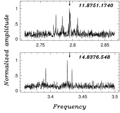
Figure 7: Examples of type MC variables with BL2 structures. Arrow indicates the position of the (prewhitened) main pulsation component. Spectra are computed by SAM. See text for comments on the peak structures.

In order to be more specific on all five stars containing structures of type BL2, below we give a short description of their frequency spectra. In the following we use the notation $\nu_{0}$ for the main pulsation component.

11.8751.1740 – The frequency spectrum shows some PC-type remnant at $\nu_{0}$, a symmetric pair of peaks around it and an additional component further away (see Fig. 7).

14.8376.548 – The frequency spectrum shows a symmetric pair of closely spaced peaks around $\nu_{0}$ and an additional peak further away (see Fig. 7).

18.2357.757 – Classified as BL2 from the SAM analysis of set #1. From set #2 we found an additional close component, therefore the final classification has become of MC.

19.4671.684 – The frequency spectrum shows a dominantly BL2 structure, but there are additional peaks spred closely.

6.6697.1565 – The frequency spectrum shows two BL2 structures superposed, one with large and another one with small frequency separations. The closer pair has also lower amplitudes.

The remaining eight stars from the MC variables show distinct peaks without any apparent BL2-type peak structures. Representative examples of these variables are shown in Fig. 8. We see that these are indeed different from the ones generally classified as type BL.

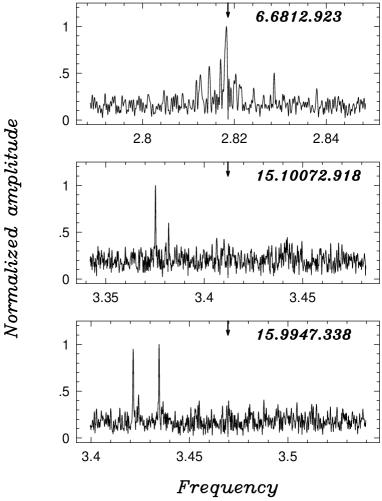
Figure 8: Examples of type MC variables without symmetric peak structures of type BL2. Arrow indicates the position of the (prewhitened) main pulsation component. Spectra are computed by SAM.

It is interesting to examine the distribution of the size and the position of the modulation components. For comparison, in Fig. 9 we show the distributions of the modulation amplitudes both for the RR1 and RR0 BL stars. It is seen that in both classes there are variables with very high modulation amplitudes, exceeding $0.1$ mag. This may correspond to $\sim 50$% and $\sim 90$% relative modulation levels for the RR0 and RR1 stars, respectively. In the other extreme, at low modulation amplitudes, we find cases near $0.01$–$0.02$ mag. From the size of the noise and the number of the data points, we expect about these amplitudes as the lowest ones to be detected in this dataset. It is important to note that current investigations by Jurcsik and co-workers (Jurcsik et al. 2005a) suggest that modulation may occur under $0.01$ mag among fundamental mode Galactic field Blazhko stars. It is clear that we need more accurate data on the LMC to check if these low modulation levels are more common also in other stellar systems.

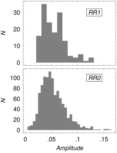
Figure 9: Upper panel: distribution of the ‘b’ modulation amplitudes of the 99 RR1 stars shown in Table 7. In the case of BL2 stars the amplitudes of both side peaks are included. Lower panel: as in the upper panel, but for the ‘V’ modulation amplitudes of the 731 RR0 stars of A03.

Concerning the relative positions of the modulation components, in Table 8 we show the number of cases obtained in the different datasets with the larger modulation component preceding the main pulsation component. We see that in the case of RR1 stars we have nearly 50% probability that this happens. This result is basically independent of BL type, color and extent of the dataset. We recall that A03 derived 75% for this ratio for the RR0 stars in the LMC.

Table 8: Positions of the larger modulation amplitudes

Type	Color	$N_{+}$	$N_{\rm tot}$	$N_{+}/N_{\rm tot}$
BL1	‘r’	12	32	0.38
	‘b’	18	44	0.41
	‘SAM’	21	46	0.46
BL2	‘r’	13	22	0.59
	‘b’	21	46	0.46
	‘SAM’	24	53	0.45

Notes: Dataset #2 is used; $N_{+}=$ number of cases when the larger modulation amplitude has a frequency greater than that of the main pulsation component; $N_{\rm tot}=$ total number of BL stars identified in the given color.

The present study has largely extended the range of the BL periods known for RR1 stars. The distributions of the modulation frequencies for the RR1 and RR0 stars are shown in Fig. 10. Although the sample is much smaller for the RR1 stars, it is clear that there are more stars among them with short modulation periods than among the RR0 stars. Nevertheless, we should mention that Jurcsik et al. (2005a, b) found very short modulation periods also among RR0 stars, albeit in the Galactic field (i.e., SS Cnc and RR Gem with $P_{\rm BL}=5.3$ and $7.2$ d, respectively). It is also noted that the considerable surplus in the RR1-BL stars with long modulation periods can be attributed only partially to our lower limit set on $f_{\rm BL}$. We find that among the $34$ stars contributing to the first bin in Fig. 10 for the plot of RR1 stars, there are only $11$ with $1.0/T<f_{\rm BL}<1.5/T$ and $16$ with $1.0/T<f_{\rm BL}<2.0/T$. This implies a significant peak in the distribution function for $f_{\rm BL}<0.005$ even with the omission of these objects with very long modulation periods. The lack of such a peak for the RR0 stars might indicate a difference in this respect between the RR0 and RR1 BL stars, but, due to the low sample size for the RR1 stars, we would caution against jumping to this conclusion.

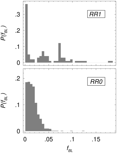
Figure 10: Upper panel: distribution of the modulation frequencies of the 99 RR1 stars shown in Table 7. Lower panel: as in the upper panel, but for the modulation frequencies of the 731 RR0 stars of A03.

5.2 Miscellaneous variables

In Table 9 we list the properties of the variables showing frequency spectra difficult to classify. We see that in most cases the detections are barely above the noise level. Therefore, we cannot exclude that at least some of these variables will turn out to be single-periodic RR1 stars, when more accurate data will be available. In the column “Comments” we show the period ratios in cases when some sort of double-mode pulsation can be suspected (without suggesting that those variables are indeed of double-mode ones).

Table 9: List of miscellaneous stars

MACHO ID	$\nu_{0}$	$\nu_{MI}$	SNR	Source	Comments
10.3916.849	3.1389921	1.2070180	6.61	SAM
11.8745.899	3.3176002	4.7867033	6.79	SAM	$\nu_{0}/\nu_{MI}=0.6931$
13.5719.713	3.0220610	3.9155071	6.96	SAM	$\nu_{0}/\nu_{MI}=0.7718$
18.2717.787	2.8643249	4.9297051	6.55	SAM	$\nu_{0}/\nu_{MI}=0.5810$
18.3202.956	2.2855398	5.1908177	6.96	r
19.3575.541	3.3698536	0.5856270	7.91	SAM
3.7451.484	3.3048194	2.7630866	7.85	b	$\nu_{MI}/\nu_{0}=0.8361$
80.6348.2470	2.9571188	1.2069597	6.65	SAM
80.7558.650	2.7828759	0.8240633	6.99	r
81.8519.1395	2.9463890	0.8372214	6.96	r
9.5004.750	3.2877325	0.1604569	7.42	SAM
9.5122.363	3.1033541	4.1679579	6.82	SAM	$\nu_{0}/\nu_{MI}=0.7446$
9.5241.382	3.1777911	1.3826455	6.79	SAM

Notes: $\nu_{0}$ denotes the frequency (in [d^-1]) of the main pulsation component, $\nu_{MI}$ stands for the frequency of the miscellaneous component with SNR given in the next column. Interesting period ratios are given in the comment lines.

6 Conclusions

This work has been motivated by an earlier result of Alcock et al. (2000) on the low incidence rate of the first overtone Blazhko RR Lyrae (RR1-BL) stars in the LMC. They derived a rate of 4% for these stars, which is a factor of three lower than that of the fundamental mode (RR0) stars (see Alcock et al. 2003). Soszyński et al. (2003) obtained a somewhat higher rate of 6% from the OGLE database. However, Alcock et al. (2000) used MACHO ‘r’ data that have somewhat lower signal-to-noise ratio for the objects of interest, and, in addition, the data analyzed then, spanned a shorter time base than the ones available now. This suggests that the incidence rate could be higher than the one deciphered earlier. In a full utilization of all available data we employed a spectrum averaging method that enabled us to increase the detection rate by 18% in comparison to the best single color (i.e., ‘b’) rates.

The main conclusion of this paper is that indeed, the incidence rate of the RR1-BL stars in the LMC is higher than previously derived from nearly the same database. Even though the rate is 7.5% now, it is still significantly lower than that of the RR0 stars. This latter rate is 12%, that we also expect to increase slightly when the same method as the one used in this paper on RR1 stars is to be employed also on RR0 stars. This means, that, at least for the LMC, we can treat as a well-established fact that RR1-BL stars are significantly less frequent than their counterparts among the RR0 stars. It is also remarkable that after filtering out the main pulsation component, the highest amplitude peak appears with equal probability at both sides of the frequency of the main pulsation component. We recall that in the case of RR0 stars there is a 75% preference toward the higher frequency side. The smallest modulation amplitudes detected for RR1 stars are near $0.02$ mag. For the larger sample of RR0 stars this limit goes down to $0.01$ mag. The relative size of the modulation may reach $90$% for RR1 stars, whereas the same limit is only $50$% for the RR0 stars. Furthermore, RR1-BL stars have a relatively large population of short-periodic ($P_{\rm BL}<20$ d) variables, which region is nearly empty for the RR0 stars in the LMC.

Since the underlying physical mechanism of the BL phenomenon is still unknown, it is also unknown if these (and other) observational facts will put strong (or even any) constraints on future theories. Nevertheless, since these statistics are based on large samples, their significance is high and surely cannot be ignored in the theoretical discussions. For example, we note that the very existence of BL1 stars puts in jeopardy the present forms of both currently available models (magnetic oblique rotator/pulsator by Shibahashi 2000; non-radial resonant model by Nowakowski & Dziembowski 2001; see however Dziembowski & Mizerski 2004).

- (1) Alcock, C. et al., The macho collab., 1999, PASP, 111, 1539
- (2) Alcock, C. et al., The macho collab., 2000, ApJ, 542, 257 (A00)
- (3) Alcock, C. et al., The macho collab., 2000a, AJ, 119, 2194
- (4) Alcock, C. et al., The macho collab., 2003, ApJ, 598, 597 (A03)
- (5) Alcock, C. et al., The macho collab., 2004, AJ, 127, 334
- (6) Dziembowski, W. A. & Mizerski, T., 2004, Acta Astr., 54, 363
- (7) Nowakowski, R. M. & Dziembowski, W. A., 2001, Acta Astr., 51, 5
- (8) Jurcsik, J. Sódor, Á., Váradi, M., Szeidl, B. et al., 2005a, A&A, 430, 1049
- (9) Jurcsik, J., Szeidl, B., Nagy, A. & Sódor, Á., 2005b, Acta Astr., 55, 303.
- (10) Kovács, G., Zucker, S. & Mazeh, T. 2002, A&A, 391, 369
- (11) Kovács, G., 2005, A&A, 438, 227
- (12) Kurtz, D. 1985, MNRAS, 213, 773
- (13) Mizerski, T. 2003, Acta Astron., 53, 307
- (14) Moskalik, P. & Poretti, E. 2003, A&A, 398, 213
- (15) Shibahashi, H. 2000, ASP Conf. Ser., 203, 299
- (16) Smolec, R., 2005, Acta Astron., 55, 59
- (17) Soszyński, I., Udalski, A., Szymański, M. et al., 2000, Acta Astron., 50, 451
- (18) Soszyński, I., Udalski, A., Szymański, M. et al., 2002, Acta Astron., 52, 369
- (19) Soszyński, I., Udalski, A., Szymański, M. et al., 2003, Acta Astron., 53, 93
- (20) Szeidl, B. 1988 in ‘Multimode Stellar Pulsations’, Kultúra, Konkoly Observatory, Budapest; Eds.: G. Kovács, L. Szabados, B. Szeidl, p. 45.
- (21) Szeidl, B. & Kolláth, Z., 2000, ASP Conf. Ser., 203, 281
- (22) Udalski, A., Szymański, M., Kubiak, M., 1997, Acta Astron., 47, 319