OB Stars in the Solar Neighborhood I: Analysis of their Spatial Distribution

Abstract

We present a newly-developed, three-dimensional spatial classification method, designed to analyze the spatial distribution of early type stars within the 1 kpc sphere around the Sun. We propose a distribution model formed by two intersecting disks -the Gould Belt (GB) and the Local Galactic Disk (LGD)- defined by their fundamental geometric parameters. Then, using a sample of about 550 stars of spectral types earlier than B6 and luminosity classes between III and V, with precise photometric distances of less than 1 kpc, we estimate for some spectral groups the parameters of our model, as well as single membership probabilities of GB and LGD stars, thus drawing a picture of the spatial distribution of young stars in the vicinity of the Sun.

1 Introduction

With the naked eye it is possible to observe that the brightest stars in the sky are mainly distributed along two great circles forming an angle of about $20\arcdeg$ between them: the Milky Way and a tilted strip known as the Gould Belt (Herschel, 1847; Struve, 1847; Gould, 1879). Later studies found out that the GB is better described as a planar distribution of O and B stars in the solar neighborhood, inclined with respect to the Galactic plane (Lesh, 1968; Stothers & Frogel, 1974).

Although this structure doesn’t show an uniform stellar distribution (the bulk of the stars tend to form aggregates around the regions of Orion and Sco-Cen, among others), the fact that the kinematic behavior of the GB members is different from that of the LGD stars of the same spectral types (Lesh, 1968; Stothers & Frogel, 1974), and that several features of the local interstellar medium such as dust (Gaustad & Van Buren, 1993), neutral hydrogen (Lindblad, 1967; Lindblad et al., 1973) or molecular clouds (Dame et al., 1993) seem to be associated with the system of OB stars, we can assume that we are witnessing a star-forming process with a spatial scale length of 1 kpc. Thus, the concept of a star formation complex proposed by Efremov (1978, 1995) and recently revised by Elmegreen et al. (2000) appears to have in the GB its closest example.

Extensive reviews covering the history of research about the GB and describing the present state of our knowledge and understanding of this structure can be found in Pöppel (1997) and Grenier (2004).

1.1 A review of classification methods in literature

When it comes to studying the stellar component of this complex, the first and most serious problem that arises is to isolate the GB members from the stars belonging to the LGD field. This problem has been addressed before by many authors, the proposed methods being intimately related to their a priori hypotheses about the geometry of the system (usually, either a real belt or toroid, or a disk).

The first and most intuitive way of facing the problem that we came across in scientific literature is, once the position of the stars in a three-dimensional frame (normally, Cartesian Galactic coordinates $X$,$Y$,$Z$) is known, then all or some of the three possible projections (i.e., $Y$ vs. $X$, $Z$ vs. $X$ and $Z$ vs. $Y$) can be plotted, in order to choose limit distance criteria according to the apparent position of the GB in each of the coordinate planes. This commonly translates into defining a ”box” for each projection inside which every star belongs to the GB. Examples of this procedure can be found in Pellegatti Franco (1983), Westin (1985), Lindblad et al. (1997) and Moreno et al. (1999) among others. The greatest advantage of this method is its simplicity, but undoubtedly there is an important contamination of LGD stars in the final selection of GB members, specially in the diffuse zone of intersection between the two systems.

A second method is based on maximum likelihood analysis of the star density projected over the celestial sphere. Assuming that the stars of both the GB and the LGD are confined around two great circles in the Galactic latitude vs. longitude projection, the proposed stellar density of both structures decreases as an exponential function of the angular distance to those great circles. The analysis of those distributions provides information about the structure of the GB and the LGD without having to assign individual membership probabilities to the stars. Fine examples of this method are seen in Comerón et al. (1994), Torra et al. (1997) or Fernández (2005).

Those two lines of attack have in common in that the classification is based on strictly spatial criteria, obtained from two-dimensional projections. But, while the first yields only a raw approximation to the GB members, the second allows to estimate some structural parameters of the system, such as its inclination with respect to the Galactic plane, the longitude of its ascending node, its angular thickness and the fraction of stars belonging to each group. On the other hand, this model is based on two rather hard structural hypotheses:

1. The Sun is located in the center of the GB

2. The GB stars are distributed along a toroidal geometry

Such restrictions impose a limitation on other possible three-dimensional scenarios (such a disk-like structure), that would be difficult to adjust within these premises.

Therefore, providing that we know the distances of the stars, the need for a three-dimensional analysis arises. Here, we can take advantage of all the spatial information at our disposal and to expand the number of possible structural scenarios. The first to propose such an approach to the problem were Stothers & Frogel (1974). They assumed that both the GB and the LGD could be represented by two crossed planes around which the stars are distributed by a law decreasing with the distance to each mid plane, the parameters that define them being estimated by least-square fitting. Then, they assign individual membership to the stars according to their vertical distance $Z$ (in Cartesian Galactic coordinates) to each plane; i.e. a star belongs to the GB if its $Z$ distance to the GB mid-plane is smaller than that to the LGD mid-plane, and vice-versa. All this procedure is nested within an iterative algorithm that re-calculates the equation of the planes and re-assigns memberships until the convergence is reached. The disadvantages of this method are that it produces ”artificially sharp surfaces on the systems on the sides that face each other” (Stothers & Frogel, 1974), and that, as it seems unavoidable for any separation method based only in the spatial distribution of the stars, in the region of intersection between the planes the discrimination cannot be fully trusted.

1.2 Objectives

We have developed a new three-dimensional spatial classification method which allows us to estimate the mean planes that define the GB and the LGD, and the single star probabilities of belonging to either of them. Essentially, as in Stothers & Frogel (1974), we obtain the mean planes by least-squares fitting, but instead of simply assigning membership by a $Z$-coordinate criterion, we define a parametric stellar density distribution for each plane that makes it possible to work with membership probabilities. An essential contribution is the introduction, for the first time in this kind of studies, of the detection of outliers in the sample, and the analysis of their effect on the estimation of the model parameters.

In this article, we shall give a detailed description of our classification method (Sections 2.1 and 2.2), then we shall test its validity and limitations using synthetic samples (Section 2.3). A real sample of OB stars from the Hipparcos Catalogue (ESA, 1997), with precise photometric distances will be compiled in Section 3, and then we shall apply our separation algorithm to this sample in order to obtain the structural parameters that best describe the GB and the LGD (Section 4). Finally, we shall develop a correction of completeness to enhance our results (Section 5), and we shall resume the most important conclusions of this article in Section 6.

2 Classification method

2.1 The spatial model

The most restricting simplification that we must assume to build our model is that the stars belonging to the GB and the LGD are concentrated along two planes, the distance $d$ of their members to the mean planes being distributed according to a parametric probability density function (pdf). Two types of functions have been tested in this study: exponential and Gaussian pdfs.

$$\phi(d)=\frac{1}{h}e^{-\frac{d}{h}}~{};~{}~{}~{}\phi(d)=\frac{1}{h}e^{-(\frac{d^{2}}{2h^{2}})}$$ (1)

where $h$ is, respectively, the scale height and the half-width. An exponential pdf, aside from being very practical in terms of calculus, is commonly used for describing the vertical distribution of the stars in models of galactic disks (Bahcall & Soneira, 1984; Gilmore, 1984; Chen et al., 2001). However, it has the annoying characteristic of having a non-continuous derivative at its maximum. Thus, an apparently more realistic function such as a Gaussian pdf has been tested too.

Using heliocentric Galactic rectangular coordinates ($X$,$Y$,$Z$), where $X$ is positive in the direction of the Galactic center, $Y$ in the direction of Galactic rotation and $Z$ perpendicular to the Galactic plane so that they form a direct frame, the mean planes may be expressed by the standard Cartesian plane equation

$$a_{1}X+a_{2}Y+a_{3}Z+a_{4}=0$$ (2)

Then, the distance of any point ($x$,$y$,$z$) to the plane is simply

$$d=\frac{|a_{1}x+a_{2}y+a_{3}z+a_{4}|}{\sqrt{a_{1}^{2}+a_{2}^{2}+a_{3}^{2}}}.$$ (3)

Although this definition is useful in computational terms, a better geometrical understanding is provided by the following parameters: the inclination with respect to the Galactic plane ($i$), the Galactic longitude of the ascending node ($\Omega$) and the vertical distance to the Sun ($Z_{0}$), where

$$\begin{array}[]{l}a_{1}=\sin i\sin\Omega\\ a_{2}=-\sin i\cos\Omega\\ a_{3}=\cos i\\ a_{4}=-a_{3}Z_{0}\end{array}$$ (4)

if we normalize the $a_{i}$ to $\sqrt{a_{1}^{2}+a_{2}^{2}+a_{3}^{2}}=1$ (see Figure 1 for a visualization of the geometrical scheme of the problem).

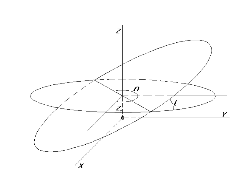
Figure 1: Geometrical scheme of the two intersecting planes model. See the text for explanation of the symbols.

2.2 Statistical procedure

The classification of the star sample will be done according to the principles of Bayesian discriminant analysis, a description of which may be found in Cabrera-Caño & Alfaro (1990).

If we know all the parameters that define the planes, we can construct the pdfs for the GB and the LGD, $\phi_{GB}$ and $\phi_{LGD}$, from equation (1). Then, if we know the a priori probability of any star being a GB member, $f_{GB}$, the Bayes theorem can be written as

$$p_{GB}=\frac{f_{GB}\phi_{GB}}{f_{GB}\phi_{GB}+(1-f_{GB})\phi_{LGD}}$$ (5)

where $p_{GB}$ is the a posteriori probability of belonging to the GB for a star with a known distance to both planes. Thus, following the Bayes minimum error rate decision rule, we may classify a star as a GB member if $p_{GB}>0.5$, or as a LGD member if $p_{GB}\leq 0.5$.

Obviously, since we lack a pre-classified sample from which to obtain the parameters of the planes, we must follow an iterative procedure to estimate them. Departing from some reasonable initial values of $i$, $\Omega$ and $Z_{0}$ for the planes of the GB and the LGD, of $f_{GB}$ and of the scale heights $h_{GB}$ and $h_{LGD}$, that we use for the initial classification of the sample, we obtain a first result that serves to calculate a second estimate of all the parameters, which we then use as the initial values for a third estimation; and so on, iteratively, until we reach the convergence.

2.2.1 Main algorithm

The estimation algorithm is divided into the following steps:

1. The scale heights $h_{GB}$ and $h_{LGD}$ as parameters of the pdfs are simply estimated as the variance of the distances of the stars to the corresponding plane.

2. $f_{GB}$ is estimated as the ratio of the obtained number of GB members to the sample size.

3. The parameters of the planes are obtained by orthogonal least squares fitting. If ${\mathbf{r}}_{i}=(x_{i},y_{i},z_{i})$ is the position vector of the star $i$, we first calculate the mean position vector $\overline{{\mathbf{r}}}$ and the matrix of moments ${\mathbf{M}}$

   $$\overline{{\mathbf{r}}}=\frac{1}{N}\sum_{i=1}^{N}{\mathbf{r}}_{i}\\ \\$$ (6)

   $${\mathbf{M}}=\frac{1}{N}\sum_{i=1}^{N}({\mathbf{r}}_{i}-\overline{{\mathbf{r}}})^{T}({\mathbf{r}}_{i}-\overline{{\mathbf{r}}})$$ (7)

   where $N$ is the number of stars in the classified sample. We solve the eigenvalues equation

   $$\det({\mathbf{M}}-\lambda{\mathbf{I}})=0$$ (8)

   and then we solve for the eigenvector ${\mathbf{u}}$

   $$({\mathbf{M}}-\lambda_{0}{\mathbf{I}}){\mathbf{u}}=0$$ (9)

   where $\lambda_{0}$ is the smallest root of equation (8). Then the fitted orthogonal least squares plane equation may be written

   $${\mathbf{u}}\cdot({\mathbf{r}}-\overline{{\mathbf{r}}})=0$$ (10)

   and from the values of the $a_{i}$ coefficients, we can compute $i$, $\Omega$ and $Z_{0}$, according to equation (4).

This iterative algorithm is fully nested within a bootstrap structure in order to simultaneously obtain error estimates of the model parameters. Thus, the procedure is performed once with the true sample, and then it is repeated 99 more times with pseudo-samples of the same size built by choosing stars at random -repetition being allowed- from the original batch.

2.2.2 Detection of outliers

An important issue remains, though, which is that of the possible contamination of our sample by outliers that don’t belong to either of our two distributions as we have defined them, i.e., that they are too far away from the mean planes and cause deviations in the estimation of the parameters. This implies that an outlier will be found in zones of low density of probability in the sampling space (Cabrera-Caño & Alfaro, 1985). Since we know the pdfs for the GB and the LGD, we can evaluate the total density $D$ in the position of any star of the original sample:

$$D=f_{GB}\phi_{GB}+(1-f_{GB})\phi_{LGD}$$ (11)

We consider as an outlier any star located in a point in space where the density D is lower than a certain threshold, which indicates the regions so far from the mid planes that we may safely consider that stars in these zones do not belong to our distributions. We have found after the examination of our system that a conservative value of $D<10^{-3}$ fulfills our requirements to eliminate most of the possible outliers. All the outliers are removed from the sample before the iterative process begins and the new parameters are estimated. Once the new result has been obtained, we reintroduce the full sample and obtain the outliers as defined by the new planes, thus beginning a second iterative procedure that will lead to the final estimation of the parameters without contamination by outliers.

2.3 Stability analysis

In order to study the behavior of our model, we have built a series of test samples with known parameters that we may compare with those estimated by the algorithm. These samples respond to the simplifications assumed in our model, i.e. they are two clouds of points distributed along two crossed mid planes. In rectangular coordinates ($X$,$Y$,$Z$), the points are originally distributed at random in the $XY$ plane, while their height $Z$ follows an exponential pdf (equation 1). Then, each cloud of points is rotated as a whole by an angle $i$, and then by an angle $\Omega$, and displaced a vertical distance $Z_{0}$ (their values being obviously different for each set of points). Finally, a distance limit $r$ to the whole sample is chosen ($\sqrt{a_{1}^{2}+a_{2}^{2}+a_{3}^{2}}\leq r$). The number of points in each sample is about 700 to 800, which are the remaining ”stars” after the distance cut (each sample originally has 1000 points which, to avoid undesired border effects, extend beyond the 1 kpc limit when we assign their random distances). A typical test sample after the separation procedure is shown in Figure 2, where 5% of the LGD stars and 7.5% of the GB stars have been misclassified, mainly in the zone of intersection between the planes. Some isolated stars far away from the mid plane of their corresponding distribution have also been misclassified.

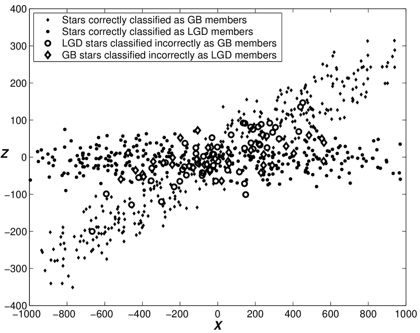
Figure 2: Classification of a synthetic sample of stars with parameters $i_{GB}=17\arcdeg$, $\Omega_{GB}=285\arcdeg$ and $Z_{0}^{GB}=-10$

In Figure 3 we plot the results of one series of tests of a simulated GB for each of the model parameters. Each point in the top panel of Figure 3 represents the mean result of the first iteration procedure for a hundred samples with fixed true parameters ($i_{GB}=17\arcdeg$, the dashed line in the figure). The initial values introduced at the beginning of the process are equal to the true parameters of the synthetic samples, except for the one whose behavior we want to analyze; in this case, $i_{GB}$ . For each of these points we observe that:

1. Convergence is reached typically in less than 10 iterations, for a precision of $0.01\arcdeg$.

2. The mean error of $i_{GB}$, estimated by the bootstrap procedure, is $0.2\arcdeg$, so the number of iterations actually needed for a significative convergence is very low.

We also observe that the first iterative process leads to an underestimation of the inclination if the initial value is lower than the real one, or to an overestimation if the initial value is greater the true inclination. A balance is achieved by the reintroduction of the full sample for a second iteration under the newly estimated parameters, which leads to a new, more refined detection of the outliers. For instance, for an initial value of $i_{GB}=14\arcdeg$, an initial convergence is reached at $i_{GB}=16.4\arcdeg$; introducing $i_{GB}=16.4\arcdeg$ as the initial value leads to a final convergence of $i_{GB}=16.8\arcdeg$. Only two steps have been necessary to stabilize the result, this being the typical behavior in all the tests performed.

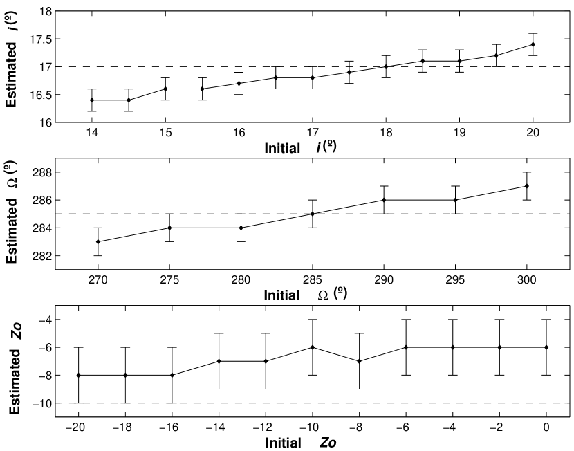
Figure 3: Estimation tests for a synthetic GB with the same parameter values as in Figure 1 (marked here by dashed lines). Each point represents the mean estimation of 100 tests with the correspondent initial value

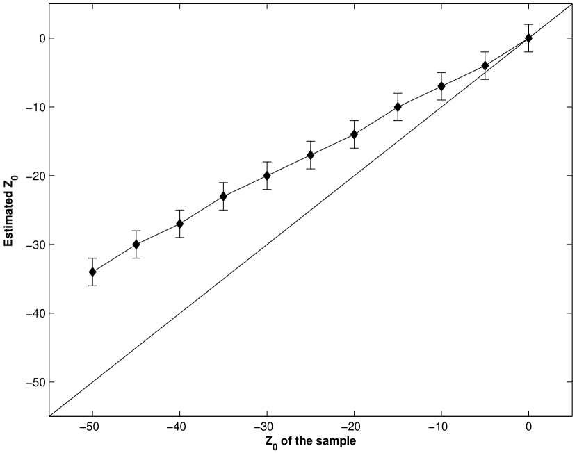
Figure 4: Estimation tests for a synthetic GB with different values of $Z_{0}$. Each point represents the mean estimation of 100 tests with the correspondent true value of the sample

Similar tests for $\Omega$ and $Z_{0}$ are shown in the middle and bottom panels of Figure 3, respectively. While the results for the longitude of the ascending node are even more precise than those obtained for the inclination (convergence is reached at $\Omega_{GB}=285\arcdeg\pm 1\arcdeg$ for a true value of $\Omega_{GB}=285\arcdeg$), an underestimation -in absolute value- of the vertical distance to the Sun is observed (convergence is now reached at $Z_{0}^{GB}=-6\pm 2$ pc for a true value of $Z_{0}^{GB}=-10$ pc). This being the parameter of the plane the most sensible to the dispersion of the stars, it seems unavoidable that we must cope with a certain bias in the estimation of $Z_{0}$. In order to evaluate the magnitude of this systematic difference we have performed some additional tests, whose results are shown in Figure 4. A hundred aleatory samples have been built for each value of $Z_{0}^{GB}$ from 0 to 50, then we have run the program to estimate $Z_{0}^{GB}$ and its error for each case. We represent their mean values in the figure, from which we can see how the estimation of $Z_{0}^{GB}$ is affected by a systematic bias of around $30\%$.

We must note that similar tests performed systematically for $Z_{0}^{LGD}$ show that there is no such a bias in the case of the LGD (or, at least, it is smaller than the random errors in the estimation), probably due to its negligible inclination. This points out that it is the geometry of the problem which is responsible for such behavior of our algorithm, and thus any pdf that we consider as a model for the vertical distribution of the planes does not alter this bias. We have corroborated that this is true by simulating the LGD and the GB systems with a Gaussian vertical distribution of the stars, and then performing the same tests with a Gaussian pdf model in our program. The results are consistent with the ones obtained working with exponential distributions, i.e., the LGD shows no significative bias in $Z_{0}^{LGD}$, and $Z_{0}^{GB}$ is affected by a systematic bias of around $35\%$.

When the simultaneous convergence of all the parameters ($i$, $\Omega$, $Z_{0}$ and $h$ for both planes, and $f_{GB}$) is sought, again only about ten iterations for the first loop and two or three for the second loop are needed, thus confirming the stability of the model.

We want to remark the importance and the uniqueness of the detection of outliers in our procedure. Stars located in the extremes of the sample distribution may have a great weight in the estimation of the model parameters, but according to their low probability of belonging to the model distribution, they must be considered as probable outliers and thus eliminated from the process. This purge of outliers leads to quite robust results, which is essential when dealing with a system such as the GB, whose spatial distribution cannot be delimited without a certain degree of uncertainty.

3 Star sample

We have selected a star sample from the Hipparcos Catalog (ESA, 1997) with spectral types from O to B6 and luminosity classes III, IV and V. The spectral types listed in the Hipparcos Catalog are a compilation from different sources; thus, a lack of homogeneity in the precision of the spectral type or the luminosity class may be present in the data. There are not systematic studies devoted to analyze the reliability of the spectral information contained in the catalog. The closest work to such an analysis has been performed by Abt (2004), who obtained and classified spectra for 584 stars belonging to A supplement to the bright star catalog. The comparison between this classification and that in the Hipparcos Catalog yields that the estimated error in the spectral classification is $\pm 1.2$ subtypes, and that a $10\%$ of the listed luminosity classes may be wrong. In this paper, the spectral classification is only used as a rough estimate of the stellar ages. Thus, the uncertainties in the spectral classification will not have any influence in the main results of our study.

For each star, the following data were chosen:

• HIP, Hipparcos identifier number.

• Trigonometric parallax $\pi$ (mas)

• Standard error in trigonometric parallax, $\sigma_{\pi}$ (mas)

• Right ascension for the epoch J1991.5 in IRCS (degrees)

• Declination for the epoch J1991.5 in IRCS (degrees)

Also, $uvby\beta$ Strömgren photometry data from the catalog of Hauck & Mermilliod (1998) were used to calculate the photometric distance of every star in the sample through the Balona & Shobbrook (1984) calibration.

Since the relative error ($\sigma_{\pi}/\pi$) of the distances estimated by Hipparcos parallaxes grows with the trigonometric distance ($1/\pi$), we have decided to keep the trigonometric distance for a star only if the relative error in its parallax is lower or equal to a $10\%$ (which corresponds approximately to distances closer than 100 pc from the Sun); otherwise, the photometric distance is chosen. Not only the error in the Strömgren estimation is independent of the distance, but also we can see (Figure 5) that the distribution of photometric distances is very similar to the distribution of trigonometric ones, and that no systematic trends can be found. Comparison between the medians of both distance estimations for stars with a relative error in their parallaxes lower or equal to a $20\%$ yields a difference between them of merely $1\%$. This is in good agreement with the studies performed by Kaltcheva & Knude (1998), who find no significant difference between Hipparcos trigonometric distances and those obtained from $uvby$ and $H_{\beta}$ photometry. Thus, we rest assured that the use of Strömgren photometric distances will not harm the precision of our three-dimensional picture of the solar neighborhood.

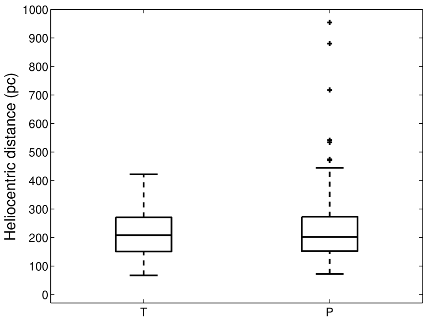
Figure 5: Boxplot comparison between Hipparcos trigonometric distances (T) and photometric distances in the Strömgren system (P) for stars with a relative error in the parallax lower or equal to a $20\%$

As we said, part of our sample has been selected with a relative error in its parallax lower or equal to a $10\%$. While the distance bias due to the non-linear relationship between parallax and distance is negligible if $\sigma_{\pi}/\pi$ is smaller than a $10\%$ (Arenou & Luri, 1999), the Lutz-Kelker bias (Lutz & Kelker, 1973) caused by truncating a sample based on the observed parallax relative error is more difficult to evaluate and depends on the parent population, as well as on the size of the selected subsample. In our case only 28 stars (about a $5\%$ of the total sample) have been selected by the parallax criterium. Thus, although this part of the sample may be affected by the Lutz-Kelker bias, the total sample shows little contamination by this effect, so wa can assume that this truncation bias is negligible in our final selection.

Finally, we have eliminated the stars with an estimated distance greater than 1 kpc, because, according to results found in the literature, the typical maximum radius of the GB is not greater than 700 pc (Stothers & Frogel, 1974; Westin, 1985; Comerón et al., 1994; Fernández, 2005). The remaining sample is composed of 553 stars; Figure 6 represents their spatial distribution projections in the three Cartesian planes $XY$ (top panel), $XZ$ (middle panel) and $YZ$ (bottom panel).

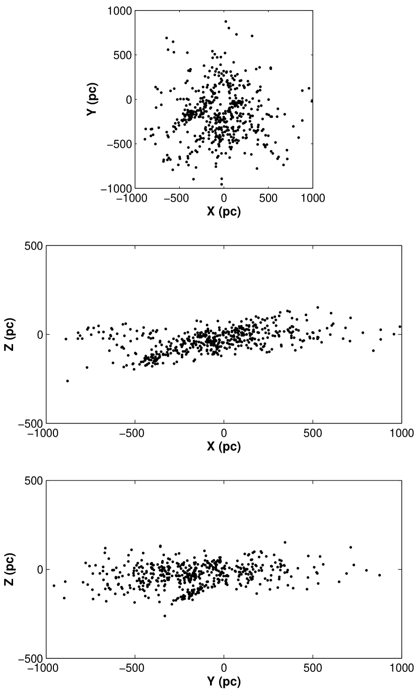
Figure 6: Spatial projections of the star sample

4 Structural results

We apply our model to the total star sample, as well as to four cumulative sub-samples that comprise all the spectral types from O to B2, B3, B4 and B5, respectively. In all cases, we find that the distribution of the stars can be satisfactorily described by our model of two intersecting planar systems, the GB presenting a remarkable inclination with respect to the LGD. While the stars belonging to the latter tend to be homogeneously distributed on the $XY$ plane, the former shows a more clumpy, filamentary structure (yet the global inclination is maintained across the whole GB system). The numerical results that fit the model planes for the cumulative samples of increasing spectral types are displayed on table 1. We have listed separately the solutions depending on whether an exponential or a Gaussian pdf has been used.

While some of the model parameters are found to be the same -within the estimated errors- regardless of the employed pdf, others show non negligible differences. Specially, the number of outliers and the fraction of stars belonging to the GB system ($f_{GB}$) display significant discrepancies. The number of outliers working with a Gaussian pdf is close to a $20\%$ of the total sample, meaning that about 100 out of 554 stars have a very low probability of belonging either to the GB or to the LGD. This fraction, though, is reduced to a $10\%$ when an exponential pdf is used. According to these results we consider that our sample is better described by an exponential law than by a Gaussian one. We must note that this cannot be extrapolated for the GB system as a whole, and thus must be seen only as the best fitting for our observational sample.

Table 1: Estimated parameters of the GB and the LGD planes

					$h_{GB}$	$h_{LGD}$	$i_{GB}$	$i_{LGD}$	$\Omega_{GB}$	$\Omega_{LGD}$	$Z_{0}^{GB}$	$Z_{0}^{LGD}$
$Sp$	$N$	$N^{\prime}$	$n$	$f_{GB}$	$(pc)$	$(pc)$	$(\arcdeg)$	$(\arcdeg)$	$(\arcdeg)$	$(\arcdeg)$	$(pc)$	$(pc)$
Exponential pdf:
O-B2	181	162	3	0.53 (0.06)	27 (4)	34 (3)	16 (2)	2 (1)	273 (7)	354 (165)	-14 (8)	-10 (8)
O-B3	301	267	2	0.54 (0.05)	27 (3)	34 (2)	14 (1)	2 (1)	278 (5)	352 (152)	-19 (10)	-10 (8)
O-B4	341	303	3	0.54 (0.05)	27 (3)	35 (2)	14 (1)	2 (1)	281 (5)	354 (154)	-17 (9)	-17 (7)
O-B5	484	433	1	0.54 (0.05)	27 (3)	35 (2)	14 (1)	1 (1)	284 (3)	356 (156)	-13 (5)	-17 (5)
O-B6	553	498	1	0.54 (0.05)	27 (3)	34 (2)	14 (1)	1 (1)	284 (3)	355 (149)	-13 (6)	-16 (5)
Gaussian pdf:
O-B2	181	144	3	0.54 (0.06)	18 (3)	23 (3)	17 (1)	1 (1)	277 (5)	346 (147)	-4 (5)	-10 (5)
O-B3	301	247	5	0.49 (0.05)	18 (2)	27 (2)	16 (1)	1 (1)	280 (3)	342 (126)	-6 (5)	-12 (4)
O-B4	341	279	2	0.48 (0.06)	18 (2)	28 (2)	16 (1)	1 (1)	280 (4)	342 (116)	-7 (3)	-14 (4)
O-B5	484	396	4	0.40 (0.04)	15 (1)	30 (2)	17 (0.4)	1 (1)	282 (2)	327 (78)	-8 (3)	-15 (3)
O-B6	553	454	4	0.37 (0.03)	13 (1)	30 (2)	17 (0.3)	1 (1)	284 (2)	321 (58)	-5 (3)	-16 (3)

Note. — $Sp$ stands for the spectral types comprised in each cumulative sample, $N$ gives the initial sample size, $N^{\prime}$ is the number of stars remaining in the sample after the elimination of outliers and $n$ is the number of iterations in the second loop needed to reach convergence (it must be noted that the initial values of the parameters given to the algorithm are the ones obtained as a result from the previous subsample, except in the O-B2 case). It must be also noted that $h$ stands for both the scale height of the exponential model, and for the half-width of the Gaussian pdf solution. Errors estimated by bootstrap are given in parentheses.

We find an inclination of the GB between $14\arcdeg\pm 1\arcdeg$ and $17\arcdeg\pm 0.3\arcdeg$ for all the samples, except for the youngest sub-sample of O-B2 stars, where the range is reduced to $i_{GB}=16\arcdeg\pm 2\arcdeg-17\arcdeg\pm 1\arcdeg$ ). It’s a smaller value than those commonly found in the literature, yet we may compare it with those estimated by Westin (1985) on table 2. In his study he estimates too a larger inclination for the youngest sample (albeit $2\arcdeg$ larger than that found for our sub-sample with the earliest spectral types). Moreover, his result for the sample ranging from 30 to 60 Myr matches the inclination of $14\arcdeg$ found for our later spectral types. Also, Torra et al. (2000a, b), from a sample of Hipparcos OB stars with Strömgren photometric distances, estimate an inclination of $22\arcdeg$ for stars younger than 30 Myr, and an inclination of $16\arcdeg$ for stars in the range of 30 to 60 Myr. It’s worth noting that in the earlier work of (Stothers & Frogel, 1974), $i_{GB}=18\arcdeg\pm 0.4\arcdeg$ for their O-B5 sample, and $i_{GB}=19\arcdeg\pm 1\arcdeg$ for an O-B2.5 subsample, yet they find for stars in a range of spectral types from B3 to B5 that $i_{GB}=16\arcdeg\pm 1\arcdeg$.

Table 2: GB plane parameters for samples of different age, from Westin (1985)

Sample Age	$i_{GB}$	$\Omega_{GB}$
$(yr)$	$(\arcdeg)$	$(\arcdeg)$
$<2\cdot 10^{7}$	$18.9\pm 1.1$	$273.2\pm 3.1$
$<3\cdot 10^{7}$	$18.1\pm 0.9$	$270.9\pm 4.3$
$(3-6)\cdot 10^{7}$	$14.3\pm 2.0$	$286.2\pm 5.7$

Comparing the values that we estimate for $\Omega_{GB}$, we see that they are in very good agreement with those of Westin (1985). The earlier spectral types present a smaller value of $\Omega_{GB}$, similar to that found by Westin (1985) for the youngest samples, while his result for the oldest age groups matches those we obtain when later spectral types are included. The values of $\Omega_{GB}=275\arcdeg-295\arcdeg$ (depending on the sample age) found by Torra et al. (2000a, b) are also in good agreement with our results. Other similar values were estimated by Torra et al. (1997), $\Omega_{GB}=278\arcdeg-290\arcdeg$, and Comerón et al. (1994), $\Omega_{GB}=284.5\arcdeg$, from OB stars of the Hipparcos proposal.

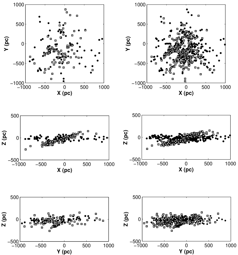
Figure 7: Classified O-B2 sub-sample (left) and full O-B6 sample (right). Black circles represent the LGD and open squares, the GB.

Even though there’s agreement in most of the estimations made by different authors of the GB geometrical parameters around a certain range of values, it is true that this range is sometimes quite large (for instance, $i_{GB}\approx 14\arcdeg$ - $22\arcdeg$). We shall venture that this isn’t only caused by the choice of different ages, spectral types or heliocentric distance limits of the star samples, but that the presence of outliers in those samples may seriously be affecting the results. It is perfectly possible that the weight of only a few stars with a low membership probability to the distribution sensibly alters the estimation, leading to unrealistic values of the parameters. Since the ”limits” of the GB constitute a very diffuse zone whose boundaries cannot be easily defined, we consider that unless outliers are purged it is not possible to characterize its spatial distribution with confidence enough as to define the series of parameters (such as the inclination or the longitude of the ascending node) that are usually employed to describe its geometry.

Our model also gives an estimation of the Sun’s distance to the Galactic plane, which oscillates between $10\pm 8$ pc (for the O-B2 and O-B3 subsamples) and $17\pm 7/5$ pc (for the O-B4 and O-B5 subsamples, respectively). Although this parameter is biased, as we had already foreseen in the simulations testing the model (the bottom panel of Figure 3, and Figure 4, perfectly illustrate that), the raw values we obtain are compatible with those found by Humpreys & Larsen (1995) from the Palomar Sky Survey star counts ($Z_{\odot}=20.5\pm 3.5$ pc), by Hammersley et al. (1995) from $2.2\mu m$ and $3.5\mu m$ maps by the DIRBE instrument of the COBE satellite and the Two-Micron Galactic Survey ($Z_{\odot}=15.5\pm 3$ pc), or by Cohen (1995) from the IRAS Point Source Catalog in $12\mu m$ and $25\mu m$ ($Z_{\odot}=15.5\pm 0.7$ pc). However, the mean age of these catalogs is much older than the young LGD we are dealing with in this work.

The comparisons of the O-B5 subsample with the analysis of a star sample of the same spectral types by Stothers & Frogel (1974), who choose an exponential-type scale height model, show an even better match with our results. They find that $Z_{\odot}=24\pm 3$ pc and that -in the sphere of 200 pc around the Sun- the scale height of the LGD is $h_{LGD}=45\pm 18$ pc. Their estimation of the scale height of the GB, $h_{GB}=27\pm 4$ for stars closer than 200 pc and $h_{GB}=27\pm 1$ for stars closer than 800 pc, is in perfect agreement with our results. A more recent study on the disk O-B5 stellar population by Maíz-Apellániz (2001), using a highly developed Gaussian model, concludes that $Z_{\odot}=25.2\pm 2.0$ pc and $h_{LGD}=62.8\pm 6.4$ pc. Also, working with a self-gravitating isothermal disk model, he finds that $Z_{\odot}=24.2\pm 2.1$ pc and $h_{LGD}=34.2\pm 3.3$ pc, the latter value matching almost exactly our estimation of $h_{LGD}=35\pm 2$ for the O-B5 subsample with an exponential model. It is worth noting too that our earlier O-B2 subsample yields similar results to those obtained by Reed (1997, 2000) for an O-B2 disk using also an exponential model ($h_{LGD}=45\pm 20$ pc, $Z_{\odot}=9.5\pm 3.5$ pc).

We also estimate a small inclination for the LGD between $1\arcdeg\pm 1\arcdeg$ and $2\arcdeg\pm 1\arcdeg$, which -although its high uncertainty points out that it isn’t a very significative value- is somewhat greater than that by Hammersley et al. (1995) of $0\arcdeg.40\pm 0\arcdeg.03$. It is small enough, though, to make $\Omega_{LGD}$ remain not well defined, hence the large ($150\arcdeg-160\arcdeg$) uncertainty that we should expect for pure geometrical reasons when $i_{LGD}$ is close to zero, as it is the case.

Figure 7 displays the three possible projections for the classified O-B2 sub-sample (left panels) and the complete O-B6 sample (right panels) for the exponential pdf solution. The inclination of the GB is clearly seen in the $XZ$ plane (middle panels); it is also interesting to observe the irregular spatial distribution of the GB in the $XY$ plane (top panels) presenting clustering and filamentary structures, in contrast with the more homogeneous LGD distribution. That is better seen in Figure 8, where the spatial density distribution of both systems has been plotted. Note the clustering of the GB density distribution (left panel), the most prominent feature being located in the Orion region in the third Galactic quadrant.

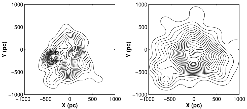
Figure 8: Spatial star density of the GB (left) and the LGD (right) for the classified full sample.

5 Correction of completeness

The spatial density distribution of the LGD shows that the star density decreases with the increasing distance to the Sun, as we may see in the right panel of Figure 8. Certainly, such a distribution is not what we should expect on this region of the solar neighborhood. If we assume that on this scale the LGD should present a homogeneous star density, it is evident that what we observe in the figure is due to the incompleteness of our sample. Thus, under this hyphotesis, we can use the two-dimensional density of the LGD as a measure of the star field incompleteness in the working region. This density map may be seen as a sort of ”flat field” used for completeness correction, that will allow us to improve the structural analysis of the GB.

We have to note, though, that the interstellar medium extinction pattern may also be playing an important role in the modulation of the observed density structure. While the effect of distance on the incompleteness of the sample is indistinctly reflected on the density correction for the GB and the LGD, the extinction pattern could show different features for both systems. Thus, this ”flat field” correction must be considered as a first approach to the problem of incompleteness, and not as a definitive solution. However, the main properties of the dust distribution in the solar neighborhood (see Pöppel 1997 for a detailed discussion) makes us confident in the reliability of this approach.

5.1 Model parameters

Dividing the GB star density by the LGD star density would be enough to provide a relative density that would enhance the structures that belong solely to the GB, but we can take a further step and introduce this correction in our model. We thus modulate the weight of any star (which originally was the probability of belonging to the correspondent plane) by a completeness function that simply is the inverse of the LGD star density in the $(x,y)$ position of the star, evaluated by a Gaussian kernel.

Following again the iterative process for the O-B6 full sample with an exponential pdf model, we reach convergence in the following values:

• $f_{GB}=0.58\pm 0.06$

• $h_{GB}=31\pm 4$ pc

• $h_{LGD}=34\pm 5$ pc

• $i_{GB}=14\arcdeg\pm 1\arcdeg$

• $i_{LGD}=2\arcdeg\pm 2\arcdeg$

• $\Omega_{GB}=287\arcdeg\pm 6\arcdeg$

• $\Omega_{LGD}=352\arcdeg\pm 28\arcdeg$

• $Z_{0}^{GB}=-15\pm 12$ pc

• $Z_{0}^{LGD}=-12\pm 12$ pc

We observe that, within the error margin, the results are similar to those we had previously obtained (table 1). This indicates that even with an incomplete sample, the structural results estimated by our model are still valid.

5.2 Spatial structure

In Figure 9 we draw the nearest OB associations over the star density maps of the GB. As we see, the correction of completeness removes the contribution to the central peak by the effect of the decreasing star density with the heliocentric distance, allowing the region around Scorpio to stand by itself. Also, the Orion peak moves farther away, towards the position of Ori OB1.

It is important to note that this is the first time that a correction of completeness has been implemented in order to compensate for the always incomplete samples constructed to study the spatial distribution of the GB. No significant difference can be found in the estimation of the GB structural parameters, even though the new density map of its spatial distribution (Figure 9, right panel) shows important modifications of the original distribution (Figure 9, left panel) in the $XY$ plane. This is probably due to the geometry of the system, dominated by the GB’s inclination with respect to the Galactic plane (hence, the $Z$ vertical distribution playing a fundamental role) and by the outer parts of the structure, better separated from the LGD. Nonetheless, the completeness correction is tremendously reassuring if we consider the difficulty of gathering a complete enough sample of GB stars, and it lets us look confidently at our results. It also provides a most interesting picture of the effects of incompleteness on the clumpy $XY$ distribution of the GB, and its correspondence with OB associations.

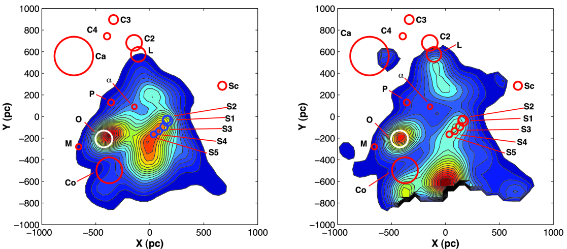
Figure 9: Spatial star density of the GB before (left) and after (right) the completeness correction. The circles represent the pre-Hipparcos OB associations, as listed by de Zeeuw et al. (1999). The letters stand for: Sco OB2₁ (S1), Sco OB2₂ (S2), Sco OB2₃ (S3), Sco OB2₄ (S4), Sco OB2₅ (S5), Col 121 (Co), Ori OB1 (O), Mon OB1 (M), Per OB2 (P), $\alpha$ Per ($\alpha$), Cam OB1 (Ca), Lac OB1 (L), Cep OB2 (C2), Cep OB3 (C3), Cep OB4 (C4), Sct OB2 (Sc)

5.3 Associations

Since the work by Blaauw (1965), it is known that the young associations Sco-Cen, Per OB2, and Ori OB1 are part of the GB, while the field members could have originated from the disruption of oldest groups (Pöppel 1997). In fact, these three groups are well inside the typical radius of the GB, but most of the associations found within 1 kpc in the radius around the Sun seem to be out of the classical borders of the belt.

After the flat fielding correction of the density map of the GB, we observe how new clumps appeared (Fig. 9, right panel). Within the uncertainty in the estimated distances of the associations, these clumps can be linked to well known and cataloged associations (e.g. de Zeeuw et al 1999). The GB membership of the associations is not only defined by the position of the centroid (a single point), but by a relative maximum in the stellar density pattern of the GB. Thus, young associations as Cam OB1, Lac OB1, Col 121 and a clump (at $X=0$, $Y\sim-600$ pc) that’s connected to the Vela rift are likely GB members, extending the GB frontiers to larger distances.

Perhaps the most striking result is the inclusion of some Vela groups as probable GB members. We wonder -after a suggestion from the referee- if this presence could be a spurious effect generated by the ”flat field” correction due to a different reddening pattern in the GB and the LGD. However, Vela is located close to the line of nodes in which the GB and the LGD coexist. Thus, the dust distribution is probably shared in this region by both systems, so it is not likely that it is responsible for the introduction of this maximum.

6 Conclusions

We have developed a new three-dimensional spatial classification method to estimate the structure of the GB and the LGD, working with single star membership probabilities. This method, although based in a model of two planar intersecting systems, allows for a greater variety of spatial configurations than other classification techniques found in literature, which is helpful in order to understand the complex structure of the GB. We have tested this method with artificial samples, and then we have applied it to a true sample of OB stars in the sphere of 1 kpc around the Sun. As a result, we have obtained that the distribution of young stars in the solar neighborhood is dominated by two different systems: the LGD and the inclined structure of the GB. Our hypothesis of two intersecting disks has been quite effective in order to characterize both systems for their study, and although we have found that the GB is a clumpy, filamentary structure, we have successfully estimated through our model the geometrical parameters of the GB and the LGD, which are in good agreement with earlier estimations by other authors. The inclination of the GB is found to be between $i_{GB}=14\arcdeg-17\arcdeg$.

Also, a completeness correction has demonstrated that the estimation of the global parameters that define our GB model were not affected by the decrease of the star density with the heliocentric distance, providing robust parameter estimators. Yet this correction effectively refines the projected spatial density distribution of the GB on the $XY$ plane, removing false substructures and enhancing the true ones, some of which we may relate to the nearby OB associations.

References

- Abt (2004) Abt, H.A. 2004, ApJS, 155, 175
- Arenou & Luri (1999) Arenou, F., & Luri, X. 1999, ASPC, 167, 13
- Bahcall & Soneira (1984) Bahcall, J.N., & Soneira, R.M. 1984, ApJS, 55, 67
- Balona & Shobbrook (1984) Balona, B.A., & Shobbrook, R.R. 1984, MNRAS, 211, 375
- Blaauw (1965) Blaauw, A. 1965, Koninkl. Ned. Akad. Wetenschap., 74, No. 4
- Cabrera-Caño & Alfaro (1985) Cabrera-Caño, J., & Alfaro, E.J. 1985, A&A, 150, 298
- Cabrera-Caño & Alfaro (1990) Cabrera-Caño, J., & Alfaro, E.J. 1990, A&A, 235, 94
- Chen et al. (2001) Chen, B., et al. 2001, ApJ, 553, 184
- Cohen (1995) Cohen, M. 1995, ApJ, 444, 874
- Comerón et al. (1994) Comerón, F., Torra, J., & Gómez, A.E. 1994, A&A, 286, 789
- Dame et al. (1993) Dame, T.M., et al. 1987 ApJ, 322, 706
- de Zeeuw et al. (1999) de Zeeuw, P.T., Hoogerwerf, R., de Bruijne, J.H.J., Brown, A.G.A., & Blaauw, A. 1999, AJ, 117, 354
- Efremov (1978) Efremov, Yu. N. 1978, SvAL, 4, 66
- Efremov (1995) Efremov, Yu. N. 1995, AJ, 110, 2757
- Elmegreen et al. (2000) Elmegreen, B.G., Efremov, Y., Pudritz, R.E., & Zinnecker, H. 2000, in Protostars and Planets IV, eds. V. Mannings, A.P. Boss, S.S. Russell, Tucson: University of Arizona Press
- ESA (1997) ESA 1997, The Hipparcos and Tycho Catalogs, ESA SP-1200
- Fernández (2005) Fernández, D. 2005, PhD Thesis, Universitat de Barcelona, Spain
- Gaustad & Van Buren (1993) Gaustad, J.E., & Van Buren, D. 1993, PASP, 105, 1127
- Gilmore (1984) Gilmore, G. 1984, MNRAS, 207, 223
- Gould (1879) Gould, B.A. 1879, Uranometría Argentina, Result. Obs. Nac. Argentino, I, p. 354
- Grenier (2004) Grenier, I. A. 2004, preprint (astro-ph/9096)
- Hammersley et al. (1995) Hammersley, P.L., Garzon, F., Mahoney, T., & Calbet, X. 1995, MNRAS, 273, 206
- Hauck & Mermilliod (1998) Hauck, B., & Mermilliod, M. 1998, A&AS, 129, 431
- Herschel (1847) Herschel, J.F.W. 1847, Results of Astron. Observations made during the years 1834-1838 at the Cape of Good Hope, London
- Humpreys & Larsen (1995) Humpreys, R.M., & Larsen, J.A. 1995, AJ, 110, 218
- Kaltcheva & Knude (1998) Kaltcheva, N., & Knude, J. 1998, A&A, 337, 178
- Lesh (1968) Lesh, R.J. 1968, ApJS, 17, 371
- Lindblad (1967) Lindblad, P.O. 1967, BAN, 19, 34
- Lindblad et al. (1973) Lindblad, P.O., Grape, K., Sandqvist, A., & Schober, J. 1973, A&A, 24, 309
- Lindblad et al. (1997) Lindblad, P.O., Palouš, J., Lodén, K., & Lindegren, L. 1997, in Hipparcos Venice ’97, ed. B. Battrick (ESA SP-402) (Noordwijk: ESA), 507
- Lutz & Kelker (1973) Lutz, T.E. & Kelker, D.H., 1973, PASP, 85, 573
- Maíz-Apellániz (2001) Maíz-Apellániz, J. 2001, AJ, 121, 2737
- Moreno et al. (1999) Moreno, E., Alfaro, E.J., & Franco, J. 1999, ApJ, 522, 276
- Pellegatti Franco (1983) Pellegatti Franco, G. A. 1983, Ap&SS, 96, 195
- Pöppel (1997) Pöppel, W. 1997, FCPh, 18, 1
- Reed (1997) Reed, B.C. 1997, PASP, 109, 1145
- Reed (2000) Reed, B.C. 2000, AJ, 120, 314
- Stothers & Frogel (1974) Stothers, R., & Frogel, J.A. 1974, AJ, 79, 456
- Struve (1847) Struve, F.G.W. 1847, études d’Astronomie Stellaire: Sur la Voie Lactée et sur la distance des étoiles fixes, St. Petersburg
- Torra et al. (1997) Torra, J., Gómez, A.E., Figueras, F., Comerón, F., Grenier, S., Mennessier, M.O., Mestres, M., & Fernández, D. 1997, in Hipparcos Venice ’97, ed. B. Battrick (ESA SP-402) (Noordwijk: ESA), 513
- Torra et al. (2000a) Torra, J., Fernández, D., & Figueras, F. 2000, A&A, 359, 82
- Torra et al. (2000b) Torra, J., Fernández, D., Figueras, F., & Comerón, F. 2000, Ap&SS, 272, 109
- Westin (1985) Westin, T.N.G. 1985, A&AS, 60, 99