Local Voids as the Origin of Large-angle Cosmic Microwave Background Anomalies I

Abstract

We explore the large angular scale temperature anisotropies in the cosmic microwave background due to expanding homogeneous local voids at redshift $z\lesssim 1$. A compensated spherically symmetric homogeneous dust-filled void with radius $\sim 3\times 10^{2}h^{-1}$Mpc, and density contrast $\delta\sim-0.3$ can be observed as a cold spot with a temperature anisotropy $\Delta T/T\sim-1\times 10^{-5}$ surrounded by a slightly hotter ring. We find that a pair of these circular cold spots separated by $\sim 50^{\circ}$ can account both for the planarity of the octopole and the alignment between the quadrupole and the octopole in the cosmic microwave background (CMB) anisotropy. The cold spot in the Galactic southern hemisphere which is anomalous at the $\sim 3\sigma$ level can be explained by such a large void at $z\sim 1$. The observed north-south asymmetry in the large-angle CMB power can be attributed to the asymmetric distribution of these local voids between the two hemispheres. The statistical significance of the low quadrupole is further reduced in this interpretation of the large angular scale CMB anomalies.

1. introduction

Despite the success of the cold dark matter ($\Lambda$CDM) model in explaining the cosmic microwave background (CMB) anisotropy on small angular scales, the possible presence of anomalies on large angular scales in the Wilkinson Microwave Anisotropy Probe (WMAP; Bennett et al. 2003) data has triggered a debate over their origin.

The reported anomalies are as follows: the anomalously low quadrupole observed by COBE/DMR (Smoot et al. 1992) and WMAP (Bennett et al. 2003); the octopole planarity and the alignment between the quadrupole and the octopole (Tegmark et al. 2003; de Oliveira-Costa et al. 2004); an anomalously cold spot on angular scales $\sim 10^{\circ}$ (Vielva et al. 2004;Cruz et al. 2005, 2006); and an asymmetry in the large-angle power between opposite hemispheres (Eriksen et al. 2004; Hansen et al. 2004). Evidence for other forms of non-Gaussianity on large angular scales has also been reported (Chiang et al. 2004; Park 2004; Schwarz et al. 2004, Larson & Wandelt 2004). It should of course be emphasized that the significance of any one of these anomalies is at most $3~{}\sigma.$ Nevertheless, the accumulation of anomalies suggests that there may be hints of new physics to be added to the standard cosmological model. The possible implications are sufficiently important that discussion of theoretical explanations is justified.

Indeed, to explain the origin of the anomalies, various solutions have been suggested. Luminet et al.(2003) proposed a non-trivial spherical topology to explain the low quadrupole, and Jaffe et al.(2005) considered a locally anisotropic model based on the Bianchi type $\textrm{VII}_{h}$ universe to explain the quadrupole/octopole planarity and alignment. Other papers have studied the possibilities that the large-angle CMB is affected by local non-linear inhomogeneities (Moffat 2005; Tomita 2005a, 2005b; Vale 2005; Cooray & Seto 2005; Rakić et al. 2006). None of these explanations is fully satisfactory, and it is therefore useful to develop an alternative interpretation of the anomalies.

In this paper, we explore the possibility that the CMB is affected by a small number of local voids at redshifts $z\lesssim 1$. As is well known, the Rees-Sciama effect (Rees & Sciama 1968) for voids could induce an additional anisotropy on large angular scales. Thompson & Vishniac (1987) and Martínez-González & Sanz (1990) have studied the anisotropy owing to a vacuum spherical (Swiss-cheese) void using the thin-shell approximation. Panek (1992), Arnau et al. (1993), and Fullana et al. (1996) studied voids for a general spherically symmetric energy profile based on the Tolman-Bondi solution (TBS;Tolman 1934; Bondi 1947). Although the TBS is a good description of voids with a general spherically symmetric density profile, it has a drawback in that it only applies before shell crossing. In contrast, the thin-shell approximation is suitable for studying voids in the late stages of evolution. In section 2, we first derive analytic formulae for dust-filled voids in the Einstein-de Sitter background using the thin-shell approximation. In section 3, we explore a model of local voids that agrees with the observed anomalies on large angular scales. In section 4, we summarize our results.

2. Dust-filled void model

2.1. Cosmic expansion

We estimate the temperature anisotropy caused by a homogeneous thin-shell void. For simplicity, we consider a matter-dominated Friedmann-Robertson-Walker (FRW) model with zero curvature (Einstein-de-Sitter model) as the background universe. In what follows, we use units in which the light velocity $c$ is normalized to 1. In spherical coordinates $(r,\theta,\phi)$, the flat background FRW metric can be written as

$$ds^{2}=-dt^{2}+R^{2}(t)(dr^{2}+r^{2}d\Omega^{2}),$$ (1)

where $t$ is the time and $R$ denotes the scale factor, and $d\Omega^{2}$ is the metric for a unit sphere. Next, we consider a homogeneous spherical dust-filled void with a density contrast $\delta<0$. We assume that the size of the void is sufficiently smaller than the Hubble radius $H^{-1}$. Then, the metric of the void centered on the origin can be approximately described by the hyperbolic FRW metric as

$$ds^{2}=-dt^{\prime 2}+R^{\prime 2}(t^{\prime})(dr^{\prime 2}+R_{c}^{2}\sinh^{2}(r^{\prime}/R_{c})d\Omega^{2}),$$ (2)

where $t^{\prime}$ is the time, $R^{\prime}$ denotes the scale factor, and $R_{c}$ is the comoving curvature radius. Assuming that the curvature radius $R_{c}$ is sufficiently smaller than the void radius $r_{v}$, up to order $O((H^{\prime-1}/R_{c})^{2})$, the scale factor for the hyperbolic FRW void can be written as

$$R^{\prime}(t^{\prime})\approx\biggl{(}\frac{3}{2}\biggr{)}^{2/3}(\Omega^{\prime}H^{\prime 2})^{1/3}t^{\prime 2/3}+3\biggl{(}\frac{3}{2}\biggr{)}^{1/3}\frac{(\Omega^{\prime}H^{\prime 2})^{-1/3}}{10R_{c}^{2}}t^{\prime 4/3}.$$ (3)

In terms of the Hubble parameter contrast $\delta_{H}\equiv H^{\prime}/H-1$ and the density contrast $\delta=\rho^{\prime}/\rho-1$, equation (3) is expressed as

$$R^{\prime}(t^{\prime})\approx(1+\delta)^{1/3}\biggl{(}\frac{t^{\prime}}{t}\biggr{)}^{2/3}+\frac{\kappa}{5(1+\delta)^{1/3}}\biggl{(}\frac{t^{\prime}}{t}\biggr{)}^{4/3},$$ (4)

where $\kappa\equiv H^{-2}/(R^{\prime 2}R_{c}^{2})=(1+\delta_{H})^{2}-(1+\delta)$ is the absolute value of the curvature in unit of the background Hubble parameter $H$. Up to order $O(\kappa)$, equation (4) yields the cosmic age for the void in terms of the model parameters $\delta_{H}$ and $\kappa$ given at a specific epoch as

$$t^{\prime}=t\biggl{(}\frac{1}{1+\delta_{H}}+\frac{\kappa}{5(1+\delta_{H})^{3}}\biggr{)}.$$ (5)

2.2. Time solution

In what follows, we calculate the evolution of the internal time $t^{\prime}$ in terms of the external time $t$ for the expanding void (with a peculiar velocity) up to order $O((r_{v}/H^{-1})^{3})$. The comoving radius of the void is expressed as $r_{v}(t)$ in the external coordinates and as $r^{\prime}_{v}(t^{\prime})$ in the internal coordinates. To connect the two metrics at the shell, we require the following boundary conditions:

$$(R(t)r_{v}(t))^{2}=(R^{\prime}(t^{\prime})r^{\prime}_{v}(t^{\prime}))^{2}\biggl{(}1+\frac{R^{\prime}(t^{\prime})^{2}r^{\prime}_{v}(t^{\prime})^{2}}{3R_{c}^{2}}\biggr{)},$$ (6)

and

$$-dt^{2}+R^{2}(t)dr^{2}=-dt^{\prime 2}+R^{\prime 2}(t^{\prime})dr^{\prime 2}.$$ (7)

where we have assumed that $r^{\prime}\ll R_{c}$. Up to order $O((r_{v}/H^{-1})^{3})$, the curvature term in equation (6) is negligible. Then equation (6) and (7) yield

$$dt^{\prime}=dt\biggl{(}1-R\dot{R}r_{v}\dot{r_{v}}\delta_{H}+\frac{1}{2}\dot{R}^{2}r_{v}^{2}\delta_{H}^{2}\biggr{)},$$ (8)

where a dot means the time derivative $d/dt$. Let us assume that the expansion of the thin shell in the external coordinates is expressed as $r_{v}(t)\propto t^{\beta}$, where $\beta$ is a constant. For the Einstein-de Sitter background, the matter dominated universe expands as $R(t)\propto t^{2/3}$. Therefore, equation (8) can be explicitly written as

$$dt^{\prime}=dt\biggl{(}1-\frac{2}{3}\beta\delta_{H}\eta^{2}+\frac{2}{9}\delta_{H}^{2}\eta^{2}\biggr{)},$$ (9)

where we define

$$\eta\equiv\frac{r_{v}(t)R(t)}{t}.$$ (10)

Integrating equation (9), we find

$$t^{\prime}\approx t\biggl{(}1-\frac{2\beta}{6\beta+1}\delta_{H}\eta^{2}+\frac{2}{18\beta+3}\delta_{H}^{2}\eta^{2}\biggr{)}.$$ (11)

Note that $\delta_{H}$ and $\eta$ are functions of $t$ rather than $t^{\prime}$. As we see in the subsequent analysis, the anisotropy turns out to have a leading order of $\eta^{3}$. Therefore, omitting the curvature term in equation (6) in the process of deriving $dt^{\prime}$ can be justified.

2.3. Expansion of voids

In the Newtonian limit, the peculiar velocity of the void $v$ can be written in terms of the gravitational acceleration $g$ and the Hubble parameter $H$ and the density parameter $\Omega$ as

$$v=\frac{2fg}{3H\Omega},$$ (12)

where $f$ is written in terms of the linear growth factor $D$ and the scale factor $R$ as

$$f=\frac{R}{D}\frac{dD}{dR}.$$ (13)

Equation (13) can be approximately written as (Peebles 1980)

$$f(\Omega)\sim\Omega^{0.6}.$$ (14)

Consider a homogeneous void with an inner radius $r_{-}$ and an outer radius $r_{+}$. We assume that the mass deficiency inside the void $-m$ is equal to the mass of the wall if the contribution from the mean density is subtracted. If we assume further that the motion of the wall is described by the distance $d_{*}$ from the center of the void where the gravitational mass satisfies $M(d_{*})=m/2$, the gravitational acceleration $g$ acting on the wall is

$$g=-\frac{G(m/2)}{d_{*}^{2}},~{}~{}m=\frac{4\pi}{3}d_{*}^{3}\delta\rho,$$ (15)

where $\rho$ denotes the background density. Plugging $g$ in equation (15) into equation (12), (13), and (14), we have (Sakai, 1995, Sakai et al. 1999),

$$v=-\frac{1}{6}Hd_{*}\Omega^{0.6}\delta.$$ (16)

Assuming $d_{*}\sim r_{v}$, the power of the expansion for a compensating void is

$$\beta\approx-\frac{1}{6}\Omega^{0.6}\delta.$$ (17)

2.4. Temperature anisotropy

We denote quantities at the time the photon enters the void and those at the time the photon leaves by the subscripts “1” and “2”, respectively. Primes denote quantities measured by a comoving observer in the interior coordinate system and the unprimed quantities are measured by a comoving observer in the background universe just out of the shell of the void. The angles $\psi_{1}$, $\psi^{\prime}_{1}$, $\psi^{\prime}_{2}$, and $\psi_{2}$ are defined by reference to figure 1.

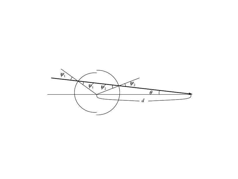
Figure 1.— Cross section of a spherical void through the plane in which the photon path and the line of sight to the void center lie. Here $\Psi$ is the angle between the light ray and the normal vector on the spherical void. The subscripts 1 and 2 represent the quantities at the time the photon enters and leaves, respectively. Primed variables represent the values inside the void.

To calculate the energy loss, we apply two local Lorentz transformations at each void boundary. The first is to convert the photon four-vector momentum in the comoving frame in the background universe to the frame in which the shell is at rest. The second is to convert it to the frame in the comoving frame inside the void.

The four-vector momentum of the photon that enters the void is

$$\mathbb{k}_{1}\equiv E_{1}\left(\begin{array}[]{c}1\\ \cos\psi_{1}\\ \sin\psi_{1}\\ 0\end{array}\right),$$ (18)

where $\psi_{1}$ is the angle between the normal vector of the void shell and the spatial three-vector of the momentum. After the photon passed the shell, the four-vector is converted to

$$\mathbb{k}^{\prime}_{1} \equiv E_{1}^{\prime}\left(\begin{array}[]{c}1\\ \cos\psi^{\prime}_{1}\\ \sin\psi^{\prime}_{1}\\ 0\end{array}\right)$$ (23)

$$= E_{1}\left(\begin{array}[]{c}\gamma_{1}\gamma_{1}^{\prime}[1+(v_{1}-v_{1}^{\prime})\cos\psi_{1}-v_{1}v_{1}^{\prime}]\\ \gamma_{1}\gamma_{1}^{\prime}[\cos\psi_{1}+(v_{1}-v_{1}^{\prime})-v_{1}v_{1}^{\prime}\cos\psi_{1}]\\ \sin\psi_{1}\\ 0\end{array}\right),$$ (28)

where $v_{1}$ and $v_{1}^{\prime}$ are the velocities of the void shell at the time $t=t_{1}$ and $\gamma$ factors are defined as $\gamma_{1}=1/(1-v_{1}^{2})^{1/2}$ and $\gamma_{1}^{\prime}=1/(1-v_{1}^{\prime 2})^{1/2}$. When the photon reaches the far edge of the shell, the four-vector momentum becomes

$$\mathbb{k}_{2}^{\prime}\equiv\frac{R_{2}^{\prime}}{R_{1}^{\prime}}E_{1}^{\prime}\left(\begin{array}[]{c}1\\ \cos\psi_{2}^{\prime}\\ \sin\psi_{2}^{\prime}\\ 0\end{array}\right).$$ (29)

As the photon leaves the shell, the four-vector momentum is converted to

$$\mathbb{k}_{2} \equiv E_{2}\left(\begin{array}[]{c}1\\ \cos\psi_{2}\\ \sin\psi_{2}\\ 0\end{array}\right)$$ (34)

$$= \frac{R_{2}^{\prime}}{R_{1}^{\prime}}E_{1}^{\prime}\left(\begin{array}[]{c}\gamma_{2}\gamma_{2}^{\prime}[1+(v_{2}-v_{2}^{\prime})\cos\psi_{2}^{\prime}-v_{2}v_{2}^{\prime}]\\ \gamma_{2}\gamma_{2}^{\prime}[\cos\psi_{2}^{\prime}+(v_{2}-v_{2}^{\prime})-v_{2}v_{2}^{\prime}\cos\psi_{2}^{\prime}]\\ \sin\psi_{2}^{\prime}\\ 0\end{array}\right).$$ (39)

The velocities of the void are

$$v_{i} = R\frac{dr_{v}}{dt}\bigg{|}_{t=t_{i}}=\beta\eta(t_{i})$$ (40)

$$v_{i}^{\prime} = R^{\prime}\frac{dr^{\prime}_{v}}{dt^{\prime}}\bigg{|}_{t^{\prime}=t_{i}^{\prime}},$$ (41)

where $i=1,2$. From the connection conditions (6) and (7), and equation (9), up to order $O(\eta^{3})$, $v_{i}^{\prime}$ can be calculated as

$$v_{i}^{\prime}(t_{i}) = \biggl{(}1-\frac{2}{9}\eta_{i}^{2}\kappa_{i}\biggr{)}\biggl{\{}\biggl{(}1+\frac{2}{3}\beta\delta_{Hi}\eta_{i}^{2}-\frac{2}{9}\delta_{Hi}^{2}\eta_{i}^{2}\biggr{)}\biggl{(}v_{i}+\frac{2}{3}\eta_{i}\biggr{)}$$ (42)

$$- \frac{2}{3}\eta_{i}(1+\delta_{Hi})\biggr{\}},$$

where $\eta_{i}\equiv\eta(t_{i})$and $\delta_{Hi}\equiv\delta_{H}(t_{i}),\kappa_{i}\equiv(1+\delta_{Hi})^{2}-(1+\delta(t_{i}))$. Using the Friedmann equation, the parameters at $t=t_{1}$ can be written in terms of those at $t=t_{2}$ as

$$1+\delta_{1}=\frac{H_{2}^{2}}{H_{1}^{2}}\biggl{(}\frac{R_{2}^{\prime}}{R_{1}^{\prime}}\biggr{)}^{3}(1+\delta_{2}),$$ (43)

and

$$\kappa_{1}=\frac{H_{2}^{2}}{H_{1}^{2}}\biggl{(}\frac{R_{2}^{\prime}}{R_{1}^{\prime}}\biggr{)}^{2}\kappa_{2}.$$ (44)

From the geometry of the void in the internal comoving frame, the relation between the void radius $r_{v1}^{\prime}$ and $r_{v2}^{\prime}$ is approximately given by

$$r_{v1}^{\prime}\sin{\psi_{1}^{\prime}}\approx r_{v2}^{\prime}\sin{\psi_{2}^{\prime}}.$$ (45)

The relation between the time $t_{1}$ and $t_{2}$ can be written as

$$\int_{t_{1}^{\prime}}^{t_{2}^{\prime}}\frac{dt^{\prime}}{R^{\prime}(t^{\prime})}\approx r_{v1}^{\prime}\cos\psi_{1}^{\prime}+r_{v2}^{\prime}\cos\psi_{2}^{\prime}.$$ (46)

The energy loss suffered between times $t_{1}$ and $t_{2}$ by a CMB photon that does not traverse the void is

$$\biggl{(}\frac{E_{2}}{E_{1}}\biggr{)}_{\textrm{no void}}=\frac{1+z_{1}}{1+z_{2}},$$ (47)

where $z_{1}$ and $z_{2}$ are redshift parameters corresponding to $t_{1}$ and $t_{2}$, respectively. The ratio of the temperature change for photons that traverse the void to that for photons that do not traverse the void is

$$\frac{\Delta T}{T}=\biggl{(}\frac{E_{2}}{E_{1}}\biggr{)}_{\textrm{void}}\frac{1+z_{2}}{1+z_{1}}-1.$$ (48)

Equations (4-7), (9),(11),(18)-(30), and (32) can be solved recursively using $\eta_{2}$ as a small parameter.

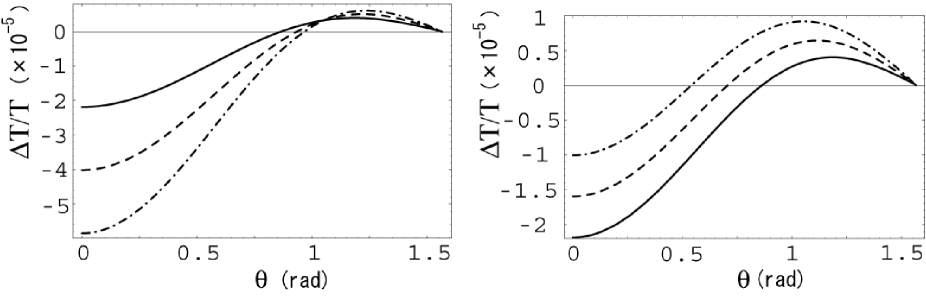
Figure 2.— The temperature anisotropy for a void with $r_{v}=340h^{-1}$Mpc, $\delta=-0.3$ and the size/distance parameter $w=1$ is plotted as a function of the subtending angle $\theta$ for various parameters that control the second order effects Left:($\epsilon,\xi$)=(0,0) (full curve), ($0.1,0$) (dashed curve), and ($0.2,0$) (dashed-dotted curve). Right:($\epsilon,\xi$)=($0,0$) (full curve), ($0,0.05$) (dashed curve), and ($0,0.1$) (dashed-dotted curve).

After a lengthy calculation, neglecting the terms of order $O(\kappa^{2})$, we find

$$\frac{\Delta T}{T} = \frac{8}{81}\eta_{2}^{3}\cos\psi_{2}\biggl{(}-9\beta(2\delta_{H}+\delta_{H}^{2}-\kappa)-2\delta_{H}\kappa$$ (49)

$$+ 2(\delta_{H}(5-2\kappa)+7\delta_{H}^{2}+3\delta_{H}^{3}-\kappa)\cos^{2}\psi_{2}\biggr{)},$$

where $\delta_{H}\equiv\delta_{H}(t_{2})$ and $\kappa\equiv(1+\delta_{H}(t_{2}))^{2}-(1+\delta(t_{2}))$.

For $\delta_{H}=-1$ and $\kappa=0$, we recover the formula for an empty Minkowski void (Thompson & Vishniac 1987). Note that the formula can also be obtained by considering the hyperbolic vacuum limit: $\delta_{H}=0$ and $\kappa=1$. For a quasi-non-linear void, the linear approximation $\delta_{H}=-\delta/3$ holds if the background universe is matter-dominated (see Appendix). Then equation (49) yields

$$\frac{\Delta T}{T}=-\frac{8}{2187}\delta\eta_{2}^{3}\cos{\psi_{2}}\Bigl{(}243\beta-(\delta-42)\delta+\delta(12+\delta)\cos(2\psi_{2})\Bigr{)},$$ (50)

where $\delta\equiv\delta(t_{2})$. Plugging equation (17) for $\Omega=1$ into equation (50), we have a simple formula for a compensating void,

$$\frac{\Delta T}{T}\approx-\frac{4}{2187}\delta^{2}\eta_{2}^{3}\cos{\psi_{2}}(3+24\cos{2\psi_{2}}).$$ (51)

Thus, we would observe the dust-filled thin shell void as a cold spot surrounded by a slightly hot ring in the sky with an anisotropy $\Delta T/T\approx-4\delta^{2}\eta_{2}^{3}/81$ toward the center of the void. To generate an anisotropy $\Delta T/T=10^{-5}$, for a given density contrast $\delta_{0}$ at the present, the void radius should be

$$r_{v}(z=0)\approx\Bigr{(}\frac{\delta_{0}}{0.2}\Bigr{)}^{-2/3}3\times 10^{2}~{}~{}h^{-1}\textrm{Mpc},$$ (52)

where $H^{-1}_{0}=3000h^{-1}$Mpc.

From equation (51), one can see that the terms that are linear in $\delta$ cancel each other if the condition $\delta_{H}=-\delta/3$ is imposed. Therefore, we conclude that the anisotropy owing to the void is a second-order effect. To model the non-linear effects, we introduce two new parameters $\epsilon$ and $\xi$ that control the second order effect. They are defined as $\delta_{H}=-\delta/3-\epsilon\delta^{2}$ and $\beta=-\delta/6+\xi\delta^{2}$ (Morita et al. 1998, Noh& Hwang 2005). One can see in the left panel in figure 2 that increasing the value of $\epsilon$ leads to an enhancement in the redshift of photons that enter the neighborhood of the center of the void because the increase in the (absolute) curvature $\kappa$ (or equivalently the decrease in the density) allows the photons to travel through the void in a shorter time. On the other hand, increasing the value of $\xi$ leads to an enhancement in the blueshift of photons whose trajectories pass near the edge of the void. This is because an increase in the expansion rate of the void shell causes a larger difference between the gravitational potentials at the time that the photon enters and at the time that the photon leaves.

To calculate the angular power spectrum, we need the angular size $\theta$ of the void. For a void at redshift $z$ centered at an angular diameter distance $d$ from the Earth, we have

$$\psi(w,\theta)=\sin^{-1}(\sin\theta/w),$$ (53)

where the size/distance parameter is defined as $w\equiv R(z)r_{v}/d$, and $\theta$ is the angular size of the void. From equations (49), (53) and non-linear parameters $(\epsilon,\xi)$, we can analytically calculate the angular power of the anisotropy.

3. Origin of large-angle anomalies

In this section, we construct a model of local voids that can explain the observed CMB large-angle anomalies. We assume that the voids are “local” at redshifts $z\lesssim 1$.

3.1. The quadrupole/octopole alignment and planarity

Tegmark et al. (2003) have found two new anomalies on very large angular scales in the CMB map from the WMAP satellite (see also Schwarz et al. 2004; de Oliveira-Costa et al. 2004). Firstly, the preferred axis of the quadrupole is aligned to that of the octopole. Although, the definition of the “preferred axis” of these low multipoles is not unique, a simple formulation is to think of the CMB temperature fluctuation as the wave function

$$\frac{\Delta T}{T}(\hat{\textbf{n}})\equiv\Psi(\hat{\textbf{n}})$$ (54)

and find the axis $\hat{\textbf{n}}$ around which the angular momentum dispersion

$$s(\hat{\textbf{n}})\equiv\langle\Psi|(\hat{\textbf{n}}\cdot\textrm{L})^{2}|\Psi\rangle=\sum_{m}m^{2}|a_{lm}(\hat{\textbf{n}})|^{2}$$ (55)

is maximized (de Oliveira-Costa et al. 2004). The interval between the unit vectors $\hat{\textbf{n}}_{1}$ and $\hat{\textbf{n}}_{2}$ corresponding to the “preferred axes” for the quadrupole and octopole is within $\sim 10^{\circ}$(de Oliveira-Costa et al. 2004).

Another anomaly is the unusual planarity of the octopole. To measure the octopole planarity, we define the octopole concentration parameter ${\cal{T}}$ as the percentages of the octopole power that can be attributed to the modes with $|m|=3$,

$${\cal{T}}(\hat{\textbf{n}})\equiv\frac{|a_{3-3}(\hat{\textbf{n}})|^{2}+|a_{33}(\hat{\textbf{n}})|^{2}}{\Sigma_{m=-3}^{3}|a_{3m}(\hat{\textbf{n}})|^{2}}.$$ (56)

For the TOE map, choosing the preferred direction in which the angular dispersion around $z$-axis is maximal, the octopole concentration parameter is ${\cal{T}}=94\%$. The relation of the octopole planarity and the concentration to the $|m|=3$ modes is obvious because the wavenumber for the fluctuation in the spherical harmonic $Y_{3,-3}$ or $Y_{3,3}$ as a function of the polar angle $\theta$ is $k\sim 1$, corresponding to a half-wave on the meridian.

To explain the quadrupole/octopole alignment and the octopole planarity, we consider a pair of identical local voids with a separation angle between the center $\theta_{s}=50^{\circ}-60^{\circ}$ at $\hat{\textbf{n}}_{1}$ and $\hat{\textbf{n}}_{2}$. If the contribution of these cold spots is dominant over the CMB in the quadrupole and the octopole, then the preferred axis for both multipoles is parallel to $\hat{\textbf{n}}_{1}-\hat{\textbf{n}}_{2}$ for which the angular momentum dispersion parallel to the rotation axis is maximum. Therefore, the quadrupole/octopole alignment is naturally explained in such a configuration. In the coordinate system in which the $z-$axis is aligned to the preferred axis, the equator lies on the equidistant point between the two identical voids. Then the wavenumber of the fluctuation owing to the two cold spots is roughly $k\sim 1$ for the separation angle $\theta_{s}\sim 60^{\circ}$ between the void. As shown in figure 3, we find a ${\cal{T}}=99.9\%$ concentration for a separation angle $\theta_{s}=53^{\circ}$ in the preferred direction independent of the size/distance ratio $w=Rr_{v}/d$.

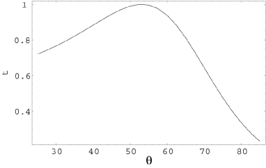
[t]

Figure 3.— The octopole concentration parameter $t$ as a function of the separation angle $\theta$ (in degree) between the pair of identical voids.

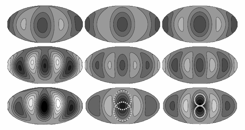
Figure 4.— The Mollweide projection maps for the cleaned CMB (Tegmark et al. 2003) (left) and those for a pair of identical voids with the size/distance ratio $w=0.9$ and the non-linear parameters $(\epsilon,\xi)=(0,0)$ (middle) and $w=0.47$, $(\epsilon,\xi)=(0.3,0)$ (right). The separation angles of the voids and the void radius are assumed to be $\theta_{s}=50^{o}$, $r_{v}=340h^{-1}$Mpc, respectively. The gray scale denotes the temperature fluctuations in which the maximum absolute value is set to $50\mu$K. The north pole is aligned to the $z-$axis for which the angular dispersion $s(\hat{\textbf{n}})$ of the quadrupole plus the octopole around the $z-$axis is maximal in the direction $(l,b)=(-110^{\circ},60^{\circ})$. The coordinate center is located at $(l,b)=(-30^{\circ},-30^{\circ})$. Top: the quadrupole maps. Middle:the octopole maps. Bottom:the quadrupole plus the octopole maps. The boundaries of the void hemispheres are denoted by small light-gray disks.

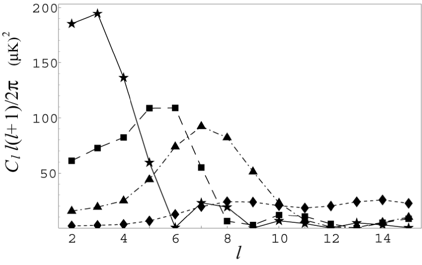
Figure 5.— Plots of the angular power $T_{l}=C_{l}l(l+1)/2\pi$ owing to a pair of identical voids with $(\epsilon,\xi)=(0,0)$ as a function of $l$ for different locations $w=0.9$ (star), $w=0.7$ (box), $w=0.5$ (triangle), $w=0.3$ (diamond) for the separation angle $\theta=50^{\circ}$. We assumed $\delta=-0.3$. and $r_{v}=340h^{-1}$Mpc. The distance to the void is given by $d\sim r_{v}/w$ at $z\sim 0$.

We can see in figure 4 that the correlation between the CMB quadrupole and the CMB octopole is large only for a cold spot centered at $(l_{c},b_{c})=(-30^{\circ},-30^{\circ})$ and a hot spot centered at $(l_{h},b_{h})=(-100^{\circ},-20^{\circ})$, suggesting that the alignment is due to these local fluctuations. Although the hot spot might be related to residual Galactic emission, it would be difficult to explain the cold spot in this way. For comparison, we have simulated the temperature anisotropies for a pair of identical voids with radius $r_{v}=340h^{-1}$Mpc for parameters $w=0.9$, $(\epsilon,\xi)=(0,0)$ and $w=0.47$,$(\epsilon,\xi)=(0.3,0)$. As shown in figure 4, we can see that the void model can generate a similar cold spot as in the observed CMB. The preferred axis is parallel to the vector that connects the centers of the voids.

3.2. The unusually cold spot

Using a wavelet technique, Vielva et al. (2004) detected an unusually cold spot in the Galactic southern hemisphere at $(l,b)=(-153^{\circ},-59^{\circ})$. The significance in the form of kurtosis on $\sim 4^{\circ}$ scales is at the $3\sigma$ (a fluke at the one in $\sim 500$) level relative to the simulation of Gaussian fluctuations. Such a cold spot can be naturally explained by a presence of a large void at $z\sim 1$ in the direction of the line of sight to the cold spot. Assuming the Einstein-de-Sitter background, for a density contrast $\delta\sim-0.3$ at $z\sim 1$ and comoving radius $r_{v}\sim 210~{}h^{-1}$ Mpc, the temperature anisotropy would be $\Delta T/T=-4\delta^{2}\eta^{3}/81\sim-10^{-5}$ in the direction of the void. The corresponding angular diameter distance at $z=1.0$ is $d=0.29~{}H_{0}^{-1}$. Then the angular radius of the void would be $\theta_{v}\sim 7^{\circ}$ and $w\sim 0.17$. For the flat-$\Lambda$ universe with $\Omega_{0}=0.3$, the corresponding angular diameter distance at $z=1.0$ is $d=0.39~{}H_{0}^{-1}$, then the angular radius of the void would be $\theta_{v}\sim 5^{\circ}$.

3.3. The north-south asymmetry

Another anomaly is the so-called north-south asymmetry: the systematic difference in the amplitudes of fluctuations on opposing hemispheres. Eriksen et al. (2004) first pointed out the asymmetry in the power for multipoles $5<l<40$ between the two hemispheres in which the “north pole” is located at $(l,b)\sim(60^{\circ},10^{\circ})$. Subsequent analyses (Hansen et al. 2004) confirmed their result.

In our void model, the asymmetry is naturally explained by the asymmetric distribution of voids on the sky. As shown in figure 5, the pair of voids at $w=0.9$ contributes for multipoles $l=2-5$ and voids at $w<0.7$ contributes for higher multipoles $l>5$ because the corresponding angular scale is $l\sim\pi/\tan^{-1}w$. The number $N$ of voids that contribute to the CMB large-angle power should be small because the asymmetry in the power falls off as $1/\sqrt{N}$.

3.4. The low quadrupole

The origin of the anomalously low quadrupole has been extensively discussed since it was first observed by COBE/DMR (Smoot et al. 1992). The WMAP team argued that the low quadrupole requires a selection at the one in 143 level (Bennett et al. 2003). However, recent studies based on Bayesian or frequentist analyses have shown that the statistical significance is actually much less than previously claimed (Tegmark et al. 2003, Efstathiou 2004). The key issue is the modeling of the foreground properties. Even though the observed power is low, most of the power may be hidden inside the Galactic foregrounds. The uncertainty in the amplitude of the cosmological background near the Galactic plane will generally lower the statistical significance of the observed power.

In a similar manner, the statistical significance of the low quadrupole can be further reduced in our void model. Consider a pair of voids with identical angular radius $\theta_{v}=\sin^{-1}w$. Then the portion of the sky area masked by the pair of voids is approximately $f\sim 1-\cos\theta_{v}$. For $w=0.7$, we have $\theta_{v}=44^{\circ}$ and $f\sim 25\%$ which is larger than the portion of the WMAP sky masks such as Kp0, Kp2 and Kp4 (Bennett et al. 2003). Therefore, we expect a further reduction in the statistical significance of the quadrupole if the pair of the voids is located sufficiently near to the Earth.

However, one may object that the amplitude enhancement would require an unusual cancellation between the intrinsic and the void-induced quadrupoles. This difficulty may be circumvented by the following argument. In the standard $\Lambda$CDM model, the adiabatic large-angle anisotropy $l<5$ owing to the “late” integrated Sachs-Wolfe (ISW) effect (redshift effect for a void) partially cancels the “ordinary” Sachs-Wolfe (OSW) effect (Hu & Sugiyama 1995). As we have seen in the previous section, the photon that traverses a point near the center is redshifted. Thus, the presence of the void may provide a further cancellation between the ISW effect and the OSW effect. A quantitative estimate is deferred to a later analysis.

4. Summary and Discussion

In this paper, we have explored the temperature anisotropy owing to dust-filled homogeneous local voids at $z\lesssim 1$ in the flat FRW universe. Local voids with a comoving radius $r_{v}\sim 3\times 10^{2}h^{-1}$ Mpc and a density contrast $\delta=-0.3$ will give a cold spot with anisotropy $\Delta T/T\sim-10^{-5}$ surrounded by a slightly hotter ring. A pair of such compensated voids at distance $\sim 4\times 10^{2}h^{-1}$Mpc whose equidistant point in the direction $(l,b)=(-30^{\circ},-30^{\circ})$ can explain the quadrupole/octopole alignment and the octopole planarity, and the void at $z\sim 1$ in the direction $(l,b)=(-153^{\circ},-59^{\circ})$ can be the origin of the unusually cold spot. We also find that the north-south asymmetry can be explained by the asymmetric distribution of these local voids.

As we have shown, the temperature anisotropy owing to a dust-filled void in the Einstein-de Sitter background is proportional to $\delta^{2}r_{v}^{3}$. Assuming the CDM power spectrum for the linear perturbation, the expected temperature anisotropy owing to the void is maximum at the scale $r_{v}\sim 100h^{-1}$Mpc, because $\delta\propto r_{v}^{-2}$ for the linear regime whereas $\delta\propto r_{v}^{-1/3}$ for the non-linear regime. Thus the contribution from the single non-empty voids at the scale $r_{v}\sim 100h^{-1}$Mpc is more important than the empty voids at smaller scales.

For simplicity, we have not considered the effect of the cosmological constant. However, we expect that the change in the deceleration parameter will not dramatically alter the order of magnitude of the anisotropy although the presence of the linear ISW effect $\sim O(\delta r_{v}^{3})$ may somehow affect the factor. The amplitude owing to the second-order effect would be $\sim O(\delta^{2}r_{v}^{3})$. Even if the density contrast $\delta$ is small, the correlation between the linear ISW term and the second order term can enhance the observed signal (Tomita 2005a,2005b). The extension of our analysis to a flat-$\Lambda$ FRW background will be presented in the forthcoming paper (K.T. Inoue & J. Silk 2006, in preparation).

We did not go into details about the non-linear evolution of the voids. Our thin-shell approximation should provide a good description of voids that are sufficiently smaller than the Hubble radius in the late stages of evolution. However, in the middle stages, the density fluctuation and the peculiar velocity of the shell may depend on the initial configuration of the density and the velocity perturbation. As we have seen, the temperature anisotropy owing to a quasi-non-linear void is a second-order effect (see also Seljak, 1996; Cooray 2002; Tomita 2005a, 2005b), which may significantly enhance the anisotropy. Therefore, we need a more elaborate calculation to make a more precise prediction about the anisotropy attributed to the local voids.

We have not addressed the issue of void origin. One may find discussions of this in previous treatments of the impact of voids on small angular scale CMB observations (Griffiths et al. 2003). The voids postulated here represent the large-radius tail of the void distribution discussed in these earlier studies. They represent a non-Gaussian fluctuation distribution that is linearly superimposed on the usual scale-invariant spectrum of Gaussian adiabatic density fluctuations. Mathis et al. (2004) discussed the implications of a distribution of primordial voids for galaxy and cluster formation. There are similar implications for the large voids that we have postulated if these are part of a statistical ensemble of primordial voids. In rare regions, associated with the thin shell surrounding the voids, cluster and galaxy formation will be enhanced. In principle this will be detectable via massive clusters and galaxies at redshifts significantly larger than expected in the purely Gaussian model. Examples include detection of massive galaxies and galaxy clusters at high $z$ and massive clusters with high concentrations of dark matter. All of these cases, if confirmed, would represent potential difficulties for the standard model of primordial Gaussian fluctuations.

Another implication unique to the very large $\sim 300~{}h^{-1}$ Mpc voids postulated here concerns increased dispersion in the Hubble constant as measured both in different directions and at different redshifts (Tomita 2001). The dispersion will be positively skewed since voids tend to generate a larger Hubble constant. Moreover, the global value of the Hubble constant will be lowered. The effect could be as large as $\sim 10\%.$

So far, the large scale voids we have assumed have not been detected. In the future, the ongoing projects such as the 6dF galaxy survey (Jones et al. 2004) may detect our postulated voids (underdensity region).

Appendix A Perturbation of Hubble parameter

Let us write the Friedmann equation at a point ${\mathbf{x}}$ in a perturbed universe in terms of the scale factor $a$, the Hubble parameter $H$, the gravitational constant $G$, and the curvature $K$ as

$$H^{2}({\mathbf{x}},t)=\frac{8\pi G}{3}\rho({\mathbf{x}},t)-\frac{K({\mathbf{x}},t)}{a^{2}(t)}$$ (A1)

where the Hubble parameter $H$ is defined on a comoving slice. ¿From the perturbed equation (A1) in the Fourier space, for the flat FRW background without $\Lambda$, we have

$$2H\delta H_{\mathbf{k}}=\frac{8\pi G}{3}\delta\rho_{\mathbf{k}}-\frac{2}{3}\biggl{(}\frac{k}{a}\biggr{)}^{2}{\cal{R}}_{\mathbf{k}},$$ (A2)

where the curvature perturbation ${\cal{R}}$ is defined as

$$\delta K_{\mathbf{k}}=\frac{2}{3}k^{2}{\cal{R}}_{\mathbf{k}}.$$ (A3)

From the Poisson equation, the Newtonian gravitational potential $\Phi_{\mathbf{k}}$ is written in terms of the density contrast $\delta_{\mathbf{k}}$ as

$$\delta_{\mathbf{k}}=-\frac{2}{3}\biggl{(}\frac{k}{aH}\biggr{)}^{2}\Phi_{\mathbf{k}}.$$ (A4)

For a constant equation of state $w\neq-1$, the continuity equation gives a relation between the gravitational potential $\Phi_{\mathbf{k}}$ and the curvature perturbation $\cal{R}_{\mathbf{k}}$ as (Liddle & Lyth 2000)

$$\Phi_{\mathbf{k}}=-\frac{3+3w}{5+3w}\cal{R}_{\mathbf{k}}.$$ (A5)

From equations (A2), (A4), and (A5), we have

$$\frac{\delta H_{\mathbf{k}}}{H}=-\frac{\delta_{\mathbf{k}}}{3(1+w)}.$$ (A6)

Thus, for the matter-dominated flat FRW universe $w=0$, the Hubble parameter contrast is written as $\delta_{H}=-\delta/3$ in the linear order.

References

- (1)
- (2) Arnau, J.V., Fullana, M.J., Monreal, L. & Sáez, D. 1993, ApJ, 402, 359
- (3) Bennett, C.L. et al. 2003, ApJS, 148,1
- (4) Bondi, H. 1947, MNRAS, 107, 410
- (5) Chiang, L.-Y., Naselsky, P., & Coles, P. 2004, ApJ, 602, L1
- (6) Cooray, A. 2002, PRD, 65, 083518
- (7) Cooray,. A. & Seto, N. 2005, JCAP, 0512, 004
- (8) Cruz, M., Martínez-González E., Vielva, P., & Cayon, L. 2005 MNRAS, 356, 29
- (9) Cruz, M., Cayon, L., Martínez-González E., Vielva, P. & Jin, J. 2006, preprint (astro-ph/0603859)
- (10) de Oliveira-Costa, A., Tegmark, M., Zaldarriaga, M.,& Hamilton, A. 2004, PRD 69, 063516
- (11) Efstathiou, G. 2004, MNRAS, 348, 885
- (12) Eriksen, H.K., Hansen, F.K., Banday, A.J., Goŕski, K.M., & Lilje, P.B. 2004, ApJ, 605, 14
- (13) Fullana, M.J., Arnau, J.V., & Sáez D. 1996, MNRAS, 280, 1181
- (14) Griffiths, L., Kunz, M. and Silk, J. 2003, MNRAS, 339, 680
- (15) Hansen, F.K., Balbi, A., Banday, A.J., & Goŕski, K.M. 2004 MNRAS, 354, 905
- (16) Jones, J.H. et al. 2004 MNRAS, 355, 747
- (17) Hu, W. & Sugiyama N. 1995, ApJ, 444, 489
- (18) Inoue, K.T. & Silk, J. 2006 in preparation
- (19) Jaffe, T.R., Banday A.J., Eriksen, H.K., Goŕski, K.M., & Hansen F.K. 2005 ApJ629, L1
- (20) Larson, D.L. & Wandelt, B.D. 2004 ApJ613, L85
- (21) Liddle, R.L. & Lyth D.H. 2000 Cosmological Inflation and Large-Scale Structure (Cambridge:Cambridge Univ. Press), 99
- (22) Luminet, J.-P., Weeks, J.R., Riazuelo, A.,Lehoucq, R., & Uzan, J.-P. 2003, Nature, 425:593L
- (23) Martínez-González, E., Sanz, J.L., & Silk J. 1990, ApJ, 355, L5
- (24) Mathis, H. et al. 2004, MNRAS, 350, 287
- (25) Mészáros, A. & Molnár Z. 1996 ApJ, 470, 49
- (26) Moffat, J.W. 2005, JCAP 0510, 012
- (27) Morita, M., Nakamura, K., and Kasai, M. 1998, PRD, 57, 6094
- (28) Noh, H., & Hwang J.-C. 2005, PRD, 69, 104011
- (29) Panek, M. 1992, ApJ, 388, 225
- (30) Park, C. 2004, MNRAS, 349:313
- (31) Peebles, p.J.E. 1980, The Large-Scale Structure of the Universe (Princeton: Princeton Univ. Press)
- (32) Rakić A., Rasänän S., & Schwarz D.J. 2006, MNRAS, 369, L27
- (33) Rees, M. & Sciama D.W. 1968, Nature 217, 511
- (34) Sakai, N., 1995 PhD thesis, Waseda University
- (35) Sakai, N., Sugiyama, N., & Yokoyama J. 1999 ApJ, 510, 1
- (36) Schwarz, D.J., Starkman, G.D., Huterer, D., & Copi, C.J 2004 PRL, 93, 221301
- (37) Seljak, U. 1996, ApJ, 460, 549
- (38) Smoot, G.F. et al. ApJ, 396, L1
- (39) Tegmark, M., de Oliveira-Costa, A., & Hamilton, A.J.S. 2003, PRD 68, 123523
- (40) Thompson, K.L. & Vishniac, E.T. 1987, ApJ, 313, 517
- (41) Tolman, R.C. 1934, Proc. Natl. Acad. Sci., 20, 169
- (42) Tomita, K. 2001, Prog. Theo. Phys., 105, 419
- (43) Tomita, K. 2005a, Phys. Rev. D, 72, 043526 (erratum 2 73, 029901[2006])
- (44) Tomita, K. 2005b, Phys. Rev. D, 72, 103506
- (45) Vale, C. 2005, preprint (astro-ph/0509039)
- (46) Vielva, P., Martínez-González E., Barreiro, R.B., Sanz, J.L., & Cayon, L. 2004, ApJ, 609, 22