Dynamics and Disequilibrium Carbon Chemistry in Hot Jupiter Atmospheres, With Application to HD 209458b

Abstract

Chemical equilibrium considerations suggest that, assuming solar elemental abundances, carbon on HD 209458b is sequestered primarily as carbon monoxide (CO) and methane ($\rm CH_{4}$). The relative mole fractions of CO(g) and $\rm CH_{4}$(g) in chemical equilibrium are expected to vary greatly according to variations in local temperature and pressure. We show, however, that in the $p$ = 1–1000 mbar range, chemical equilibrium does not hold. To explore disequilibrium effects, we couple the chemical kinetics of CO and $\rm CH_{4}$ to a three-dimensional numerical model of HD 209458b’s atmospheric circulation. These simulations show that vigorous dynamics caused by uneven heating of this tidally locked planet homogenize the CO and $\rm CH_{4}$ concentrations at $p<1$ bar, even in the presence of lateral temperature variations of $\sim\!500$–1000 K. In the 1–1000 mbar pressure range, we find that over 98% of the carbon is in CO. This is true even in cool regions where $\rm CH_{4}$ is much more stable thermodynamically. Our work shows furthermore that planets 300–500 K cooler than HD 209458b can also have abundant CO in their upper layers due to disequilibrium effects. We demonstrate several interesting observational consequences of these results.

1. Introduction

Charbonneau et al. (2000) and Henry et al. (2000) discovered the first known transiting extrasolar giant planet (EGP), HD 209458b. Transits are possible if the orbital plane of the planet is tilted along our direct line of sight. The detection of HD 209458b in transit has been a watershed in the study of planets around other stars because physical properties of the planet can be inferred directly from the transit data. The planet’s orbit is nearly circular, with a period of 3.5257 days (Laughlin et al., 2005a). Furthermore, Laughlin et al. (2005b) have combined transit data with high-resolution spectra of the star to infer accurate values for the planet’s mass and radius: $M_{\rm p}=(0.69\pm 0.05)\,M_{\rm Jupiter}$ and $R_{\rm p}=(1.32\pm 0.05)\,R_{\rm Jupiter}$.

Photons from HD209458b and the transiting planet TrES-1 have recently been detected (Deming et al., 2005b; Charbonneau et al., 2005). In addition, transmission spectroscopy measurements, in which observers track changes in the star’s spectral features while the planet is in transit, have unveiled key features of the composition of HD 209458b’s atmosphere (Brown et al., 2001; Brown, 2001; Charbonneau et al., 2002; Vidal-Madjar et al., 2003, 2004). The more recent detections of transiting planets OGLE-TR-56b (Konacki et al., 2003), OGLE-TR-113b and 132b (Bouchy et al., 2004), TrES-1 (Alonso et al., 2004), OGLE-TR-111b (Pont et al., 2004), OGLE TR-10b (Bouchy et al., 2005a; Konacki et al., 2005), HD 149026b (Sato et al., 2005), and HD 189733b (Bouchy et al., 2005b) reinforce the importance of the transit method for the characterization of close-in EGP atmospheres.

HD 209458b resides in close proximity (0.046 AU) to a Sun-like star in the constellation Pegasus. The intense stellar heating of close-in EGPs drives global-scale atmospheric dynamics. As shown by Showman & Guillot (2002), Cho et al. (2003), Burkert et al. (2005), and Cooper & Showman (2005), winds of $\sim\!3000\;\rm m\;s^{-1}$ carry material across a hemisphere in only $\tau_{\rm dyn,\,h}\sim 10^{5}\;\rm sec$. Vertical transport is rapid as well, with typical wind speeds $w\sim 20\rm\;m\;s^{-1}$ at $p=1$ bar (see §6).

Theory predicts that HD 209458b is locked by strong stellar tides to a synchronously rotating state, owing to the short time for spin-orbit synchronization of a planet at 0.046 AU (see e.g., Barnes & Fortney, 2003). The planet therefore receives stellar radiation on one hemisphere only (Guillot et al., 1996; Showman & Guillot, 2002). Various effects causing deviations from synchronous rotation have been explored in the literature, such as non-zero eccentricity or substantial obliquity pumped by the presence of another planet (Laughlin et al., 2005b; Winn & Holman, 2005). However, the apparent lack of a third massive body in the system (Laughlin et al., 2005a), as well as the timing of the transit and secondary eclipse (Deming et al., 2005b), makes a large eccentricity or obliquity unlikely for this system.

We study the atmosphere under the assumption of synchronous rotation. We note, however, that deviations from a completely synchronous state are conceivable. For example, effects of atmospheric tides are important on Venus, as shown by Correia & Laskar (2001). In an order-of-magnitude calculation, Showman & Guillot (2002) suggested that atmospheric dynamics could induce deviation from synchronous rotation by up to a factor of 2. A factor of 2 is the extreme case; 10–20% deviation might be more typical. This estimate depends on the planet’s tidal dissipation factor ($Q$), as well as properties of the circulation itself and the processes transferring angular momentum and rotational kinetic energy from the atmosphere to the interior, which are highly uncertain.

The G0V primary irradiates the planet up to an extremely high effective temperature ($T_{\rm eff}\sim 1340$ K; see Iro et al., 2005) compared to the planets of our Solar System. This leads to very different chemistry than we are familiar with in planetary atmospheres. The atmosphere is primarily composed of hydrogen and helium. Carbon, nitrogen, and oxygen are all minor constituents. Despite their low abundances, these elements are important for determining the spectral characteristics of the planet because they form molecules having strong spectral signatures (Seager & Sasselov, 1998). Radiative-equilibrium calculations by Iro et al. (2005) show that in the 1 mbar to 10 bar pressure regime, which is the region of primary interest for observations, the temperature lies in the 1000–2000 K range. At these temperatures and pressures, chemical equilibrium considerations suggest that carbon on HD 209458b is sequestered primarily in carbon monoxide (CO) and methane ($\rm CH_{4}$) (Burrows & Sharp, 1999; Lodders & Fegley, 2002). These models show that CO(g) is the most stable carbon-bearing species at high temperatures and low pressures. At low temperatures and high pressures, $\rm CH_{4}$(g) is more stable thermodynamically. The oxygen not bound up in rock is present as either CO(g) or water vapor, $\rm H_{2}O$(g).

In planetary atmospheres, however, chemical equilibrium may not hold. There are several reasons for this. First, photochemical dissociation can elevate the concentrations of photochemical products above equilibrium levels (Moses et al., 2000). Prinn & Barshay (1977) note that photochemical oxidation of $\rm CH_{4}$ is a well-known source of CO in the Earth’s atmosphere. Second, impacts by meteorites, comets, etc., deposit metals and other compounds into the atmospheres of giant planets (see, e.g., Prather et al., 1978; Moses, 1992). Third, chemical reactions may not always occur quickly enough relative to dynamical mixing for chemical equilibrium to be attained (Prinn & Barshay, 1977; Smith, 1998).

Liang et al. (2004) show that the first effect—photochemical production—is unlikely to significantly alter the concentration of CO in HD 209458b’s stratosphere ($p<1$ mbar). It is unknown how much impactors have modified the composition of HD 209458b’s atmosphere during its evolution. We note, however, that calculations by Bézard et al. (2002) show that CO deposition by impactors cannot explain the observed abundance of CO ($\sim\!1$ ppb, as opposed to essentially zero in equilibrium) in Jupiter’s lower troposphere. On Jupiter, rather, disequilibrium results from convective upwelling from deep regions ($p\sim\!300$ bar), where the equilibrium abundance of CO is higher. As the reaction rates plummet with decreasing temperature and pressure in ascending fluid parcels, the CO concentration quenches to its observed value.

Photospheric pressures lie in the 10–500 mbar range for all IR wavelengths (Fortney et al., 2005; Burrows et al., 2005; Barman et al., 2005; Seager et al., 2005). If large temperature variations of 500–1000 K in this region are a reality on HD 209458b (Showman & Guillot, 2002; Cho et al., 2003; Burkert et al., 2005; Cooper & Showman, 2005), it is conceivable that chemical quenching occurs in the horizontal rather than the vertical direction. In this hypothetical scenario, fluid parcels attain chemical equilibrium on the planet’s dayside, where the temperature is high and the reaction kinetics are fast. Vigorous dynamical motions then carry these equilibrated parcels to the nightside, where they rapidly cool to temperatures where the reactions are too slow to equilibrate the system. Depending on the meteorology and variations of the chemical rates with temperature and pressure, complex lateral CO distributions could potentially result. For example, it would then be possible for CO to be abundant at the evening limb but depleted at the morning limb.

To test the hypothesis that disequilibrium processes modify the abundances of CO and $\rm CH_{4}$ in the observable atmosphere of HD209458b, we couple the reaction kinetics to a three-dimensional nonlinear model of the atmospheric dynamics. We show that at the temperatures and pressures relevant for observations of HD 209458b’s atmosphere, the timescale for CO/$\rm CH_{4}$ interconversion is everywhere long: $\tau_{\rm chem}\gg 10^{5}$ s. Disequilibrium results in regions where the timescale for advection of CO by dynamics, $\tau_{\rm dyn}$, is shorter than $\tau_{\rm chem}$. Due to uniformly large values of $\tau_{\rm chem}$ for $p<1$ bar, the simulations definitively show that quenching occurs in the vertical, not the horizontal. As on Jupiter, we find that the concentration of CO for $p<1$ bar depends on its value deeper in the atmosphere. Vertical quenching and efficient horizontal mixing lead to a high-abundance, homogeneous distribution of CO at the photosphere. As a result, in cool regions (e.g., the nightside), the CO concentration exceeds equilibrium values by many orders of magnitude.

Curiously, CO was not detected on HD 209458b in a recent ground-based search using transmission spectroscopy at $2\,\micron$ (Deming et al., 2005a). Several possible reasons for the CO null detection have been noted by the authors and others. First, CO may not be abundant in this planet’s atmosphere, though this is only possible if the planet is significantly cooler (by $\sim\!500$ K) than predicted by current radiative-equilibrium models (Burrows et al., 2004; Chabrier et al., 2004; Iro et al., 2005). Second, CO may present in the visible atmosphere in some regions but depleted at the limb (Iro et al., 2005). Third, the spectral signature of CO at the planet’s limb may be obscured either due to photochemical haze or a high-altitude silicate cloud (Fortney et al., 2003; Burrows et al., 2004). This explanation is favored by Deming et al. (2005a). It should be noted, however, that the CO null detection reported by Deming et al. (2005a) relies on the radiative-equilibrium calculations of Sudarsky et al. (2003). If unexpected opacity sources (though not necessarily clouds) play a strong role in the formation of spectral lines near $\rm 2\;\micron$, an upper limit to the CO abundance cannot be made with high confidence based on these observations. We note $\rm CH_{4}$ has not been seen on this planet either, despite attempts to detect its signature (Richardson et al., 2003b, a).

We review in §2 the theoretical reasons to expect CO in high abundance in HD 209458b’s atmosphere based on chemical equilibrium arguments. We discuss in §3 the main chemical processes involved and derive the timescale for CO/$\rm CH_{4}$ interconversion. In §4, we describe our coupling of chemistry to the atmospheric dynamics model of Cooper & Showman (2005). We present the results of these simulations in §5. We explain and interpret these results in §6, comparing our simulations to a simpler view of quenching presented by Smith (1998). We enumerate the major uncertainties in these calculations in §7. In §8, we discuss implications of this work for near-future observations of HD 209458b and other close-in EGPs.

2. Chemical Equilibrium Considerations

Prior discussions of chemistry on EGPs are based on chemical equilibrium models (Burrows & Sharp, 1999; Lodders & Fegley, 2002). Solar abundances of the elements (Anders & Grevesse, 1989; Lodders & Fegley, 1998) are generally assumed in these schemes, which perform global minimization of the Gibbs free energy of the system, often including thermochemical data for hundreds of compounds. This minimization algorithm allows the concentrations of all chemicals to be solved for simultaneously. In such thermochemical calculations, once the elemental abundances in the atmosphere have been specified, the abundances of all chemical species in the system depend solely on the local temperature and pressure (allowing for simple ideas like rainout).

Simulations by Cooper & Showman (2005) suggest that the temperature at the photosphere of HD 209458b varies across the globe from $\sim\!1000$–1500 K. Chemical equilibrium models show that at these temperatures, the atmosphere of this planet should contain appreciable quantities of CO and $\rm CH_{4}$. Lodders & Fegley (2002) show that HD 209458b’s atmosphere straddles the line of equal CO/$\rm CH_{4}$ abundance, in the absence of disequilibrium effects. The relative concentrations of CO and $\rm CH_{4}$ are strong functions of local temperature and pressure. At 1 bar, where $\rm T\lesssim 1150$ K, $\rm CH_{4}$ is the dominant carbon-bearing species (in chemical equilibrium), while CO is more abundant at this pressure for higher temperatures (T ¿ 1150 K).

In the temperature and pressure ranges of interest for this investigation, calculation of the equilibrium abundances of CO and $\rm CH_{4}$ is straightforward and reduces to several simple algebraic expressions. These expressions are used in our disequilibrium model, in which the mole fraction of CO is relaxed to its value in chemical equilibrium (see §4.2). The expressions, as we will show, include the metallicity dependence directly. This allows us to explore the sensitivity of our disequilibrium calculations to the metallicity of HD 209458b’s atmosphere, which is conceivably enhanced from that of the host star. Such enhancement is seen on Jupiter, where C, N, and probably O are several times more abundant relative to hydrogen than at the photosphere of the Sun (Atreya et al., 1999).

We define $X_{\rm i}$ to be the mole fraction of the i-th species in the system; e.g., $X_{\rm H_{2}}$ is the mole fraction of molecular hydrogen. It is given by the ratio of the partial pressure of the i-th species to the total atmospheric pressure (i.e., $X_{\rm i}=p_{\rm i}/p$). At the temperatures and pressures in this region of HD 209458b’s atmosphere, hydrogen is primarily molecular $\rm H_{2}$ [J. Fortney, private communication]. We take $X_{\rm H_{2}}=0.83$ for the $\rm H_{2}$ mole fraction throughout this paper (i.e., we assume that $\rm H_{2}$ dissociation is everywhere negligible).

Although oxygen is mostly in CO and $\rm H_{2}O$, some oxygen is also sequestered in rock, most of which forms deeper than 1 bar (Lodders & Fegley, 2002; Fortney et al., 2005). We assume 16% of the atmospheric oxygen (the maximum possible in a solar abundance mixture is in silicates. Depending on where in the atmosphere $\rm MgSiO_{3}$ condenses, this may underestimate (by $\sim\!5$%) the oxygen available to affect CO/$\rm CH_{4}$ chemistry in the region of interest.

Defining $c_{1}$ and $c_{2}$ as the mixing ratios of gaseous carbon and oxygen in the atmosphere, the mole fractions $X_{\rm CO}$, $X_{\rm CH_{4}}$, and $X_{\rm H_{2}O}$ are related through mass balance:

$$X_{\rm CH_{4}}+X_{\rm CO}=c_{1}=5.91\times 10^{-4}$$ (1)

$$X_{\rm CO}+X_{\rm H_{2}O}=c_{2}=1.04\times 10^{-3}$$ (2)

for solar metallicity. We see from equations 1 and 2 that water vapor will always be present in the system, even if 100% of the carbon is in CO, since oxygen is more abundant than carbon.

The third expression relating the quantities $X_{\rm CO}$, $X_{\rm CH_{4}}$, and $X_{\rm H_{2}O}$ derives from the equilibrium expression of the net thermochemical reaction

$$\rm CO\,+\,3H_{2}\,\leftrightarrow\,CH_{4}\,+\,H_{2}O.$$ (3)

The equilibrium expression for reaction 3, which we denote as $\rm\mathnormal{K}_{\ref{reaction:CO_CH4_H2O_equil},\,\rm eq}$, is

$$\frac{X_{\rm CO}X_{\rm H_{2}}^{3}p^{2}}{X_{\rm CH_{4}}X_{\rm H_{2}O}}=\rm exp\left[-\frac{\Delta_{f}\mathnormal{G}_{\rm CO}-\Delta_{f}\mathnormal{G}_{\rm CH_{4}}-\Delta_{f}\mathnormal{G}_{\rm H_{2}O}}{\mathnormal{RT}}\right]=\mathnormal{K}_{\ref{reaction:CO_CH4_H2O_equil},\,\rm eq}.$$ (4)

In equation 4, $p$ is atmospheric pressure [bar], $T$ is the temperature [K], and $\rm\mathnormal{R}=8.314\;J\;mol^{-1}\;K^{-1}$ is the universal gas constant. The symbols $\rm\Delta_{f}\mathnormal{G}_{\rm CO}$, $\rm\Delta_{f}\mathnormal{G}_{\rm CH_{4}}$, and $\rm\Delta_{f}\mathnormal{G}_{\rm H_{2}O}$ represent the Gibbs free energies of formation of CO, $\rm CH_{4}$, and $\rm H_{2}O$, respectively. The Gibbs free energies of formation depend on temperature sensitively but only weakly on pressure. We simply use the values at standard pressure (1 bar), which are tabulated in the NIST-JANAF Thermochemical Tables (Chase, 1998).

With the three equations 1, 2, and 4, we can solve for the three equilibrium mole fractions $X_{\rm CO}$, $X_{\rm H_{2}O}$, and $X_{\rm CH_{4}}$ as a function of atmospheric pressure ($p$) and temperature ($T$). Defining $\mathnormal{f}=K_{\ref{reaction:CO_CH4_H2O_equil},\,\rm eq}/(p^{2}X^{3}_{\rm H_{2}})$, we solve for $X_{\rm CO}$. We take the negative root of the quadratic equation, which represents the physical solution:

$$X_{\rm CO}=\frac{-b-\sqrt{b^{2}-4ac}}{2a},$$ (5)

with $a=f$, $b=-f\,(c_{1}+c_{2})-1$, and $c=f\,c_{1}c_{2}$. The other concentrations are then easily solved for using the mass balance expressions (equations 1 and 2): $X_{\rm CH_{4}}=c_{1}-X_{\rm CO}$ and $X_{\rm H_{2}O}=c_{2}-X_{\rm CO}$. The solution is valid for temperatures between 500–2500 K over a broad range of pressures in the atmosphere. It is also valid for atmospheres with enhanced or depleted C and O abundances by simply tuning $c_{1}$ and $c_{2}$ (so long as $c_{1}$ and $c_{2}$ are kept small: $c_{1},\,c_{2}\ll 0.1$).

We show in Table 1 the ratio of CO to total carbon in the atmosphere ($X_{\rm CO}\,/\,c_{1}$), assuming chemical equilibrium, for a variety of temperatures and pressures. The table shows that the CO abundance—assuming equilibrium conditions—is a strong function of pressure and especially temperature. If large temperature variations in the atmosphere are indeed a reality on HD 209458b, as predicted both in radiative-equilibrium models (e.g., Iro et al., 2005) and simulations of the atmospheric dynamics (Cooper & Showman, 2005), large gradients in the equilibrium concentrations of CO and $\rm CH_{4}$ result. We now consider disequilibrium effects, which lead to vastly different conclusions about the relative concentrations of CO and $\rm CH_{4}$ in the upper layers of this planet’s atmosphere.

3. Chemical Pathways for CO Reduction

CO concentrations above equilibrium values have been discovered both on Jupiter (Beer, 1975; Larson et al., 1978) and on the brown dwarf Gl 229B (Noll et al., 1997; Oppenheimer et al., 1998; Saumon et al., 2000). Fegley & Lodders (1996) and Griffith & Yelle (1999) show that CO disequilibrium in Gl 229B results from the inefficiency of chemical reduction of CO in regions of low temperature and pressure relative to the rate of vertical mixing. The CO seen in the spectrum of Gl 229B originates from deeper in the atmosphere, where CO is abundant in chemical equilibrium.

Similarly, Prinn & Barshay (1977) suggest that the CO detected in the troposphere of Jupiter was transported up by convection from deeper, hotter layers of the planet. Bézard et al. (2002) explore several explanations for the unexpected 1 ppb CO concentration observed on this planet. They conclude that convective mixing from deeper layers remains the most likely source of Jupiter’s tropospheric CO, although the reactions suggested by Prinn & Barshay (1977) are now thought to be too slow to explain the observed CO abundance.

We hypothesize that dynamics may drive the abundance of CO on HD 209458b away from chemical equilibrium values. To ascertain the extent to which dynamics perturbs chemical equilibrium in this atmosphere, we first calculate the timescale for the processes converting CO to $\rm CH_{4}$ and back. This depends on the chemical reactions involved. Two independent reaction pathways for the chemical reduction of CO have been considered in the literature.

The following reaction was suggested by Prinn & Barshay (1977):

$$\rm H_{2}\,+\,H_{2}CO\rightarrow OH\,+\,CH_{3}$$ (6)

This reaction is the rate-limiting step in a three-part sequence resulting in the chemical reduction of CO to $\rm CH_{4}$. These authors calculate a rate constant for reaction 6 of

$$\rm\mathnormal{k}_{\ref{reaction:Prinn}}=2.3\times 10^{-10}\,exp\left(-\frac{36,200\>K}{\mathnormal{T}}\right)\;cm^{3}\;s^{-1}.$$ (7)

Prinn & Barshay (1977) note that the other steps leading to the reduction of CO to $\rm CH_{4}$ are fast relative to reaction 6. They use equation 7 to estimate the chemical lifetime of CO in disequilibrium as a function of temperature and pressure.

Based on more recent measurements, however, Griffith & Yelle (1999) discuss that the reaction rate for reaction 6 is significantly slower than the rate assumed by Prinn & Barshay (1977):

$$\rm\mathnormal{k}_{\ref{reaction:Prinn},\>correct}=3.4\times 10^{-8}\,\left(\frac{\mathnormal{T}}{K}\right)^{-1.12}\,exp\left(-\frac{43,192\>K}{\mathnormal{T}}\right)\;cm^{3}\;s^{-1}.$$ (8)

Furthermore, as shown by Smith (1998), the convective timescale used by Prinn & Barshay (1977) to derive the quench level is incorrect because it does not account for the gradient in both the lifetime and equilibrium abundance of CO over an atmospheric scale height. Using the updated reaction rate, equation 8, and the correct timescale for convective mixing, Bézard et al. (2002) find that the reaction sequence for CO destruction suggested by Prinn & Barshay (1977) cannot explain the disequilibrium abundance of CO in Jupiter’s troposphere. A faster reaction pathway for the reduction of CO to $\rm CH_{4}$ must be sought.

Yung et al. (1988) investigate an alternative three-step process involving the methoxy radical $\rm CH_{3}O$. They argue this pathway is more kinetically favorable because the strong carbonyl ($\rm C=O$) bond in $\rm H_{2}CO$ is broken in a separate reaction step from the formation of the four C–H bonds in methane. Yung et al. (1988) propose the following three-stage reaction set:

$$\rm H\,+\,H_{2}CO\,+\,M\rightarrow CH_{3}O\,+\,M$$ (9)

$$\rm CH_{3}O\,+\,H_{2}\rightarrow CH_{3}OH\,+\,H$$ (10)

$$\rm CH_{3}OH\,+\,H\rightarrow CH_{3}\,+\,H_{2}O$$ (11)

In this sequence, the first reaction, in which the $\rm C=O$ bond is broken, is the rate-limiting step. The net reaction resulting from summing reactions 9, 10, and 11 is

$$\rm H_{2}CO\,+\,H_{2}\,+\,H\rightarrow CH_{3}\,+\,H_{2}O.$$ (12)

We derive the number density of $\rm H_{2}CO$ by assuming equilibrium with $\rm H_{2}$ and CO: $\rm H_{2}\,+\,CO\leftrightarrow H_{2}CO$, which is fast compared to reaction 9. We note also that the production of methane ($\rm CH_{4}$) from $\rm CH_{3}$ occurs with nearly 100% efficiency (Yung et al., 1988).

The rate of reaction 9 has never been measured in the laboratory, but the rate of the reverse reaction is known (Page et al., 1989):

$$\rm\mathnormal{k}^{0}_{\rm\ref{reaction:Yung1},\>R}=1.4\times 10^{-6}\;\left(\frac{\mathnormal{T}}{K}\right)^{-1.2}\,exp\left(-\frac{7,800\>K}{\mathnormal{T}}\right)\;cm^{3}\;s^{-1}.$$ (13)

Equation 13 represents the low-pressure limit of the rate of the reverse of reaction 9 in the temperature range relevant for this planet. For the high-pressure limit, we adopt equation (11) from Bézard et al. (2002):

$$\rm\mathnormal{k}^{\infty}_{\rm\ref{reaction:Yung1},\>R}=1.5\times 10^{11}\;\left(\frac{\mathnormal{T}}{K}\right)\cdot exp\left(-\frac{12,880\>K}{\mathnormal{T}}\right)\;s^{-1}.$$ (14)

The net rate constant for the reverse reaction 9,R can be expressed as

$$\rm\mathnormal{k}_{\rm\ref{reaction:Yung1},\>R}=\frac{\mathnormal{k}^{0}_{\rm\ref{reaction:Yung1},\>R}\mathnormal{k}^{\infty}_{\rm\ref{reaction:Yung1},\>R}}{\mathnormal{k}^{0}_{\rm\ref{reaction:Yung1},\>R}\,\mathnormal{n}\,+\,\mathnormal{k}^{\infty}_{\rm\ref{reaction:Yung1},\>R}},$$ (15)

where $n$ [$\rm cm^{3}\;s^{-1}$] here is the number density of molecules in the atmosphere (Bézard et al., 2002). It is related to pressure through the ideal gas equation of state.

Using the proper eddy mixing timescale for chemical quenching derived by Smith (1998), Griffith & Yelle (1999) and Bézard et al. (2002) demonstrate that the kinetic rates derived from the Yung et al. (1988) reactions fit observations of CO in disequilibrium on the brown dwarf Gl 229b and on Jupiter. As noted above, the reaction proposed by Prinn & Barshay (1977) is too slow to account for the observed concentrations of CO in these objects. We therefore follow Griffith & Yelle (1999) and Bézard et al. (2002) in this treatment and assume that the catalyzed Yung et al. (1988) reactions 9–11 are the most efficient mechanism for the conversion of CO to $\rm CH_{4}$.

For the purpose of determining the CO quench level on HD 209458b, we use the measured reaction rates (eq. 13 – 15) along with thermochemical data to determine $\tau_{\rm chem}$. This quantity, which is a strong function of both pressure and temperature, represents the timescale over which CO can remain in disequilibrium (Prinn & Barshay, 1977). Conservation of mass (eq. 1) dictates that the rate of CO destruction must equal the rate of $\rm CH_{4}$ production. So, $\tau_{\rm chem}$ also represents the timescale for conversion of $\rm CH_{4}$ back to CO. This would not be so if other molecules competed effectively for the available carbon atoms. At these pressures and temperatures, though, CO and $\rm CH_{4}$ are the predominant carbon-bearing species (see §2). Hereafter, we simply refer to $\tau_{\rm chem}$ as the CO/$\rm CH_{4}$ interconversion timescale.

The CO/$\rm CH_{4}$ interconversion timescale is given by Bézard et al. (2002):

$$\tau_{\rm chem}=\frac{X_{\rm CO}}{-\mathrm{d}X_{\rm CO}/\mathrm{dt}}=\frac{X_{\rm CO}}{\mathnormal{n^{2}\,k_{\rm\ref{reaction:Yung1}}}\cdot X_{\rm H}X_{\rm H_{2}CO}},$$ (16)

where $k_{\rm\ref{reaction:Yung1}}$ is the reaction rate of 9. An extra factor of $n$ arises in the denominator from writing the expression in terms of CO, H, and $\rm H_{2}CO$ mole fractions rather than concentrations.

As has been noted, however, only the rate of the reverse of reaction 9 has been measured. We therefore use the equilibrium constant of the chemical reaction

$$\rm CH_{3}O\,\leftrightarrow\,CO\,+\,3/2\;H_{2}$$ (17)

to express $\tau_{\rm chem}$ in terms of equation 15. The equilibrium constant of reaction 17 is

$$\rm\mathnormal{K}_{\ref{reaction:CH3O_equil},\,\rm eq}=exp\left[-\frac{\Delta_{f}\mathnormal{G}(CO)-\Delta_{f}\mathnormal{G}(CH_{3}O)}{\mathnormal{RT}}\right].$$ (18)

The Gibbs free energy of formation of $\rm CH_{3}O$ cannot be found in the JANAF tables. We use values for $\rm\Delta_{f}\mathnormal{G}(CH_{3}O)$ from Tsang & Hampson (1986).

Using these thermochemical data along with equation 15, we can express $\tau_{\rm chem}$ in a form that can be evaluated numerically:

$$\rm\tau_{chem}(\mathnormal{p}\rm,T)=\frac{\mathnormal{X}_{CO}}{\mathnormal{n}\,\mathnormal{k}_{\ref{reaction:Yung1},\>R}\cdot\mathnormal{X}_{CH_{3}O}}=\frac{\mathnormal{K}_{\ref{reaction:CH3O_equil},\,\rm eq}\cdot\mathnormal{k}_{b}\mathnormal{T}}{\mathnormal{k}_{\ref{reaction:Yung1},\>R}\,\mathnormal{X}_{\rm H_{2}}^{3/2}\mathnormal{p}^{5/2}},$$ (19)

where $k_{\rm b}$ is Boltzmann’s constant. The first equality in equation 19 is analogous to equation 16 but for reaction 9 in the reverse direction. All intermediate reactions in the system are assumed to be in equilibrium. The second equality results from substituting equation 18 in for the ratio $X_{\rm CO}/X_{\rm CH_{3}O}$.

We show values for $\tau_{\rm chem}$ in Table 2 at the same pressures and temperatures chosen in Table 1. Table 2 demonstrates that for $p<1$ bar, $\tau_{\rm chem}\gg 10^{5}\;\rm s$ for all $\rm T\leq 2000\;K$, which is an upper limit to the temperature at HD 209458b’s photosphere. This result immediately rules out horizontal quenching as an important disequilibrium process at the photosphere. The timescale for horizontal mixing $\tau_{\rm dyn,\,h}\sim 10^{5}\;s$, so that $\tau_{\rm chem}\gg\tau_{\rm dyn,\,h}$ on both the day and night sides of the planet.

Deeper down ($p>10$ bar), CO/$\rm CH_{4}$ interconversion is fast ($\tau_{\rm chem}\ll 10^{5}$ s). At this pressure, the chemical interconversion timescale is less than both the horizontal and vertical mixing times. We would therefore expect chemical equilibrium of CO/$\rm CH_{4}$ to hold in the atmosphere at $p\gtrsim 10$ bar. The top of this region ($p\sim 10$ bar) is the approximate “quench level.” Note that the precise altitude of quenching also depends on atmospheric temperature and wind speeds, which are themselves highly variable (Cooper & Showman, 2005). As a consequence, the quench level is not an exact isobar. Referencing Table 1, we see that abundant CO at the photosphere of this planet is likely because vertical transport processes are probably efficient (Showman & Guillot, 2002), and the chemical equilibrium CO concentration at the quench level is likely to be quite high.

We now discuss a coupled atmospheric dynamics and disequilibrium CO/$\rm CH_{4}$ chemistry model to predict CO concentrations for a variety of atmospheric conditions. Our simulation results (see §5) verify the general validity of these considerations.

4. Coupled Chemistry/Dynamics Model

4.1. The Atmospheric Dynamics Model

We adapt the model of Cooper & Showman (2005) to include simple carbon chemistry based on the discussions in §2 and §3. Our model employs the ARIES/GEOS Dynamical Core, version 2 (AGDC2; Suarez & Takacs, 1995). The AGDC2 solves the primitive equations of dynamical meteorology, which are the foundation of numerous climate and numerical weather prediction models (Holton, 1992; Kalnay, 2003).

The primitive equations are a simplification of the full Navier-Stokes equations of fluid mechanics, which assume hydrostatic balance of each vertical column of atmosphere. This is equivalent to assuming that the vertical acceleration is negligible compared to the buoyancy. The approximation holds in stably stratified regions for “shallow” flow, in which the vertical depth is much smaller than the horizontal extent (Kalnay, 2003, Ch. 2). Heavy irradiation from the star extends the radiative zone of this planet down to $p\sim 1$ kbar. This is $\sim\,$1/10 of the radius (Burrows et al., 2003; Chabrier et al., 2004; Iro et al., 2005), leading to a horizontal to vertical aspect ratio of about 10:1.

The AGDC2 is a finite-difference model, which discretizes the dynamical variables onto a staggered latitude-longitude C-grid (Arakawa & Lamb, 1977). The AGDC2 consists of a set of subroutines that compute the time tendencies of the prognostic variables, including the zonal and meridional winds, potential temperature (Holton, 1992, p. 52), surface pressure, and an arbitrary number of passive tracers. At each time step, the AGDC2 simply updates the time tendencies to include the effects of the dynamics. All physical tendencies (e.g., chemistry, radiation, etc.), as well as temporal and spatial filtering needed to control computational instabilities, are performed outside of the AGDC2.

It is not possible in general to find numerically stable solutions to the primitive equations without viscosity (Dowling et al., 1998). The standard approach, which we adopt here, is to add diffusive terms to the momentum, energy conservation, and tracers equations. We have experimented with the diffusion parameters, espousing the philosophy of Polvani et al. (2004) to use as weak hyperdiffusion as possible consistent with numerically stable solutions. For the simulations discussed here, we use $4^{\rm th}$-order hyperdiffusion, with coefficients set to damp grid-scale instabilities over a timescale of $\sim\!30\;\rm minutes$.

For all simulations, we take the ”top” layer of the model to be at 1 mbar. Although a proper model of the upper atmosphere would require the model top be placed at a lower pressure, we generally ignore the upper atmosphere in this work. Modeling the high atmosphere would require a proper treatment of stratospheric photochemistry and the possible effects of non-local thermodynamic equilibrium in the radiation field at sub-millibar pressures (Liang et al., 2004; Barman et al., 2002). The atmosphere spans $\sim\!15$ pressure scale heights between our input top pressure (1 mb) and the planet’s radiative-convective boundary (1 kbar). By comparison, the pressure in the Earth’s atmosphere spans only 2–3 pressure scale heights from the surface to the tropopause. We use 40 layers evenly spaced in log pressure.

We assume in this treatment that synchronous rotation holds in the convective interior. The consequences of this assumption are twofold: (1) the rotational period is fixed to the 3.5 day orbital period (leading to a moderately strong Coriolis force), and (2) heating by the star occurs on one hemisphere of the planet continually. This assumption is valid for many hot Jupiters (such as HD 209458b), which experience rapid tidal circularization of their orbits (Guillot et al., 1996). Atmospheric tides may cause the orbit to be slightly asynchronous, as noted by Showman & Guillot (2002). But large deviations from synchronous rotation are unlikely on HD 209458b without the presence of another (thus far unseen) planet (Laughlin et al., 2005a). We discuss in §7.2 that the asynchronous component (a factor of 2 in the extreme case, though more likely in the 10–20% range) will not greatly affect the outcome of our predictions for $\rm CO/CH_{4}$ chemistry (see §7). But it would be interesting in future studies to explore the dynamics of hot Jupiters under the alternate assumption of variable heating due to non-zero eccentricity, large obliquity, or strong thermal tides.

We follow Cooper & Showman (2005) for the scalar input parameters, ignoring small variations in the gravitational acceleration, heat capacity, and mean molecular weight in the atmosphere. We set these values to constants: g = $\rm 9.42\;m\;s^{-2}$, $\rm\mu=1.81\times 10^{-3}\;kg\;mol^{-1}$, and $c_{\rm p}=\rm 1.43\times 10^{4}\;J\;kg^{-1}\;K^{-1}$. The values of these constants have been chosen to be intermediate between the values they would have at 1 mbar and 3 kbar because $\rm H_{2}$ dissociation is expected to occur in the deepest layers of the model. For the chemistry, we assume hydrogen is molecular everywhere, which holds in the upper layers of interest here (see §3).

4.2. Coupling $\rm CO/CH_{4}$ Chemistry

The AGDC2 includes horizontal advection for an arbitrary number of passive tracers. We denote these as $q_{k}$, with $k=1,2,...,km$. As few as possible is desirable, as the tracer equations add appreciably to the total computations required per time step.

Tracers are passive in the sense that they are advected by the flow but do not themselves influence the dynamics. Unless interdependencies are added, the tracer solutions in the AGDC2 do not affect the other prognostic variables (or each other). The equations operating on each $q_{k}$ are of the same form as those used for potential temperature advection (Suarez & Takacs, 1995). The advection scheme is fourth-order in this version of the dynamical core.

We add CO as a passive tracer to the AGDC2. The other carbon and oxygen bearing species, including $\rm CH_{4}$, $\rm H_{2}O$, $\rm CH_{3}O$, $\rm HCO$, etc., are either very short-lived or indirectly obtainable through mass balance (eq. 1 and 2). To confirm this, we calculated lifetimes for the intermediate species in the Yung et al. (1988) sequence. These were all much shorter than our $\rm\tau_{chem}$, which describes the timescale for interconversion of CO and $\rm CH_{4}$. For the purposes of this investigation, it is sufficient therefore to consider just a single tracer.

We follow equation (2) of Smith (1998) to express the effect of the dynamics on $\rm CO/CH_{4}$ chemistry in terms of the quantities we know, $X_{\rm CO,\>eq}$ and $\tau_{\rm chem}$. The idea is to relax $X_{\rm CO}$ to its value in chemical equilibrium, $X_{\rm CO,\>eq}$:

$$\frac{DX_{\rm CO}}{Dt}=-\frac{X_{\rm CO}-X_{\rm CO,\>eq}}{\tau_{\rm chem}}.$$ (20)

We write $D/Dt$ (not $d/dt$ or $\partial/\partial t$) to emphasize we mean the total (or material) derivative, not the local derivative. As usual, the advection terms must be included when the equations are written in the Eulerian frame (Holton, 1992, p. 28–31).

In equation 20, we see that if $\tau_{\rm chem}$ is short relative to dynamical timescales, chemical equilibrium of CO will be attained in the atmosphere. In regions where $\tau_{\rm chem}$ is longer than $\tau_{\rm dyn}$, CO will not be in equilibrium. In the former case, the CO abundance will depend solely on the local temperature and pressure (which themselves vary greatly throughout the region of integration). In the latter situation, whether the actual value of $X_{\rm CO}$ is greater than or less than the equilibrium value depends on global atmospheric conditions.

In the troposphere of Jupiter, for example, $X_{\rm CO}$ is extremely high relative to $X_{\rm CO,\>eq}$ because convection mixes CO upwards from the quench level (at several hundred bars), where the equilibrium abundance of CO is appreciable (Bézard et al., 2002). The situation of HD 209458b is different; the atmosphere in the 10 mbar to 10 bar region is stable to turbulent convection due to the huge flux of stellar radiation from above (Guillot et al., 1996). As discussed by Showman & Guillot (2002), however, vertical velocities of $\sim\!20\rm\;m\;s^{-1}$ are plausible on this planet, implying vigorous vertical transport. The CO concentration for $p<10\;\rm bar$ depends critically on the vertical flow, which we will discuss in §6.

4.3. Newtonian Heating Scheme

We defer to future work the ambitious task of coupling atmospheric dynamics to a true radiative transfer code. Rather, we approximate the effects of radiation using a simple Newtonian heating prescription. In this scheme, the thermodynamic heating rate at each grid point is proportional to the difference between the prescribed 3D radiative-equilibrium temperature and the true local temperature.

As in Cooper & Showman (2005), we start with the 1D radiative-equilibrium $T(p)$ profile of Iro et al. (2005). Their radiative-equilibrium profile, which we call $T_{\rm Iro}(p)$, assumes heat redistribution over the entire globe. The calculation includes the major sources of gaseous opacity: Rayleigh scattering, collision induced absorption, bound-free and free-free absorption, molecular rovibrational bands from $\rm H_{2}O$, CO, $\rm CH_{4}$, and TiO, and resonance lines from the alkali metals. Iro et al. (2005) calculated a line-by-line solution to the monochromatic radiative transfer equation using the Goukenleuque et al. (2000) model. This code makes the two-stream approximation (see e.g., Chamberlain & Hunten, 1987), and the atmosphere is taken to be plane-parallel. We also use values published by Iro et al. (2005) for $\tau_{\rm rad}(\mathnormal{p})$, which is the radiative relaxation time constant. This is an increasing function of pressure. The value of $\tau_{\rm rad}$ is $\sim\!3$ hours at 1 mbar (which is the topmost layer of our model) and increases to $\sim\!1$ year near 10 bar.

We use the algorithm described in Cooper & Showman (2005) to calculate $T_{\rm night}(p)$ and $T_{\rm ss}(p)$ from $T_{\rm Iro}(p)$. These are the radiative-equilibrium profiles on the nightside, which receives no direct heating, and at the substellar point, where the star is directly overhead. We assume in these calculations that nightside radiative-equilibrium temperatures depend only on pressure, not longitude and latitude. In this procedure, we prescribe a temperature difference in radiative equilibrium between the substellar point and the nightside, $\Delta T_{\rm eq}(p)=T_{\rm ss}(p)-T_{\rm night}(p)$. This is an adjustable parameter, which governs the strength of the radiative forcing. Its has been chosen to be logarithmic in pressure, so the profiles converge deep in the atmosphere.

The substellar and nightside radiative-equilibrium profiles are then computed by balancing the total flux radiating to space at the top of the atmosphere. The nightside and integrated dayside contributions must sum to the known globally averaged value, $4\pi R_{\rm p}^{2}\sigma T_{\rm Iro}^{4}$:

$$4\pi R_{\rm p}^{2}\sigma T_{\rm Iro}^{4}=2\pi R_{\rm p}^{2}\sigma T_{\rm night}^{4}+R_{\rm p}^{2}\int\!\!\!\!\int_{\rm day}\sigma T_{\rm day}^{4}(\lambda,\phi)\,\rm\cos\phi\,d\phi\,d\lambda.$$ (21)

The coordinates ($\lambda,\phi$) are longitude and latitude, respectively.

The flux balance in equation 21 yields a transcendental equation for $T_{\rm night}$ at the top of the atmosphere in terms of the free parameter, $\Delta T_{\rm eq}$:

$$4T_{\rm iro}^{4}=3T_{\rm night}^{4}+(T_{\rm night}+\Delta T_{\rm eq})^{4}.$$ (22)

In equation 22, 2 factors of $T_{\rm night}^{4}$ come from the nightside; the integral over the dayside contributes 1 more factor of $T^{4}_{\rm night}$, as well as the term involving $\Delta T_{\rm eq}$. Equation 22 can be solved numerically; we use Newton-Raphson (see Press et al., 1992). $T_{\rm night}=500\;\rm K$ is the solution for $\Delta T_{\rm eq}=1000\;\mathrm{K}$ and $T_{\rm Iro}=1000\rm\;K$.

The above radiation balance is only computed once—at the top model layer—to ensure the outgoing fluxes are self-consistent. We emphasize this is not a rigorous treatment of radiation. The goal is simply to use Iro et al. (2005)’s radiative-equilibrium profile, which is one-dimensional, to prescribe the Newtonian heating rate over the model grid in a way that does not significantly alter the radiation budget of the atmosphere.

We show in Figure 1 the radiative-equilibrium profiles generated by this method from pressures of 1 mbar to 10 bars. We plot $T_{\rm Iro}(p)$ as well for comparison. The profiles plotted are for our nominal HD 209458b model, in which we have set $\Delta T_{\rm eq}=T_{\rm ss}-T_{\rm night}=1000\;\rm K$ at the top of the atmosphere (see §5 for a more complete description). We only show the profiles down to the 10 bar level because the radiative time constants deeper than that are very long ($\tau_{\rm rad}\rm\gg 10^{7}\;s$; see Iro et al. (2005)). As in Cooper & Showman (2005), we have simply turned off heating for all pressures greater than 10 bar.

4.4. Limb Effects

Figure 1.— Radiative-equilibrium $T(p)$ profiles used in the Newtonian heating scheme described in §4.3. The profiles shown are the nightside radiative-equilibrium profile (long-dashed line), Iro et al. (2005)’s globally averaged radiative-equilibrium profile (solid line), and the radiative-equilibrium profile at the substellar point (short-dashed line). At the topmost layer of the model atmosphere (1 mbar), we have set the temperature difference between the substellar point and the nightside to 1000 K. The nightside and substellar profiles are balanced so the integrated outgoing flux at the top of the atmosphere equals $4\pi R_{\rm p}^{2}\sigma T_{\rm Iro}^{4}$. The profiles converge logarithmically with increasing pressure (depth).

Two limb effects may be important at low pressures. We have not attempted here to model them in detail. But to account for them, we use a modified form of Cooper & Showman (2005), equation(2).

First, near the limb, the angle of incidence of the impinging radiation is large. The optical path length is longer in the slant geometry than at normal incidence. Hence, the stellar radiation will not penetrate as deeply near the limb but will be absorbed higher up in the atmosphere. This causes additional heating at pressures significantly less than 1 bar. Second, the star is not a point source; it has finite angular size in the planet’s sky. This creates a small region of continuous heating past the day-night terminator, which we define here as $\rm 90\arcdeg$ from the substellar point. Here, the disk of the star is partly visible.

These considerations are potentially significant for tracking the CO distribution near the photosphere because the limb is the region directly probed by transmission spectroscopy. We attempt to account for this by modifying Cooper & Showman (2005)’s equation (2). The new profile, shown in Figure 2, is identical to that of Cooper & Showman (2005) over most of the day and night sides. But it has a smoother variation of temperature across the terminator, which remains fairly hot $90\arcdeg$ away from the substellar point (where half the stellar disk is still visible). It also increases the total radiative energy in the radiative-equilibrium system, which is realistic owing to the effects described above.

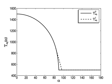
Figure 2.— The angular dependence of the 3D radiative-equilibrium profile, which is symmetric about the star-planet line. We define $\alpha$ to be the angle between the local normal vector at a particular longitude and latitude ($\lambda$, $\phi$) and a ray from the planet’s center passing through the substellar point $(\lambda=0\arcdeg$, $\phi=0\arcdeg)$. This is a slightly warmer profile near the limb than that used by (Cooper & Showman, 2005).

5. Simulation Results

For this study, we have performed a suite of simulations with different input parameters, which all support the general conclusions of this work (§8). For most of this discussion, we focus on the results of two simulations in particular. We call them the “nominal” and “cold” models, respectively. Other simulations are alluded to in this section and in §6–8.

The nominal model contains input parameters identical to those used by Cooper & Showman (2005), which are tuned for HD 209458b specifically (although the radiative-equilibrium profile has been slightly adjusted to account for limb effects; see §4.4). For the nominal model, we have used 1000 K for the radiative-equilibrium temperature difference between the substellar point and the nightside (at the top of the atmosphere, as described in §4.3). The cold model is a parameter variation on the nominal model. It is representative of an imaginary EGP that is cooler than HD 209458b. The radiative-equilibrium temperatures for the cold model are similar to those expected for the transiting planet TrES-1, which orbits a K-type star (Fortney et al., 2005; Barman et al., 2005).

We use for the cold model a new radiative-equilibrium profile, $T_{\rm Cold}(p)$. This profile is 300 K cooler at every pressure level than the profile used for the nominal model: $T_{\rm Cold}(p)=T_{\rm Iro}(p)-300\;K$. For the cold case, we have also decreased the assumed radiative-equilibrium temperature difference between the substellar point and the nightside; for this model, we use $\Delta T_{\rm eq}=700\rm\;K$. This is because we would expect cooler planets to have lower radiative forcing in general. With these adjustments, the procedure described in §4.4 was rerun on the cold profile to determine the 3D radiative-equilibrium profile for the cold case. At the topmost layer (1 mbar), the substellar and nightside profiles are $T_{\rm ss}=1085\rm\;K$ and $T_{\rm night}=385\rm\;K$, respectively.

We use the same values for the radiative relaxation time constant, $\tau_{\rm rad}(\mathnormal{p})$, as for the nominal case. For a much cooler planet than HD 209458b, $\tau_{\rm rad}(\mathnormal{p})$ would have to be re-evaluated, since radiative processes are temperature dependent. But this “cold” model is not enough colder than the nominal case for the radiative heating rates to differ by more than a factor of $\sim\!2$. All other input parameters (acceleration of gravity, heat capacity, mean molecular weight, and radius) have been kept the same as in the nominal model. It should be emphasized, therefore, that the cold model is not a model of TrES-1 or any other known EGP in particular. It is simply a parameter variation on the nominal model, which is intended to elucidate the role of atmospheric temperature in determining the $\rm CO/CH_{4}$ chemistry.

For all simulation runs presented here, the horizontal grids contain 72 points in longitude and 45 points in latitude. We have run the models for $t_{\rm sim}$ = 1000 Earth days. This is long enough for the atmosphere model to equilibrate on layers having $p\lesssim 3$ bar, since the radiative time constants are fairly short—less than a month—in this region. We have verified that the kinetic energy in these low-pressure layers does not increase with time after 500–1000 days. We use a fairly small time step for all simulations: $\rm\Delta\mathnormal{t}=50\;s$. The small time step helps to control grid-scale instabilities. We discuss these issues further in §7.

We assume zero initial zonal and meridional winds: $(u,\;v)$ = (0, 0). We also start the simulations with the temperature on every layer isothermal and equal to $T_{\rm Iro}$. We have verified that our solutions for the flow geometry—in the layers of interest here—hold even in the case of an initially strong retrograde wind (Cooper & Showman, 2005). For the initial tracer concentration, we assume chemical equilibrium of CO at $t_{\rm sim}=0$. We will discuss the effects of the initial tracer distribution in §7.3.

5.1. Temperature and Winds

Figure 3.— Temperature (grayscale) and winds (arrows) for our “nominal” model. This is a snapshot of the simulation at $t_{\rm sim}$ = 1000 days. Maximum wind speeds in each frame are (a) 6600 $\rm m\;s^{-1}$, (b) 4300 $\rm m\;s^{-1}$, and (c) 3500 $\rm m\;s^{-1}$. This is the HD 209458b nominal model, which uses parameters appropriate for the atmosphere of that planet.

We focus here on results from the nominal and cold models in the 10–1000 mbar range. These are the “visible layers” of EGP atmospheres; i.e., the layers that directly contribute to the outgoing radiation from the planet to space. The results of our integrations for the nominal model can be seen in Figure 3. Figure 3 spans about 5 scale heights in pressure, encompassing the region crucial for observations of close-in EGPs. Despite adjustments to the cooling scheme (see §4.4), the temperatures, wind speeds, and flow geometry of the nominal model are broadly consistent with simulations published by Cooper & Showman (2005).

Strong temperature contrasts on isobars are evident in the simulation for all three layers shown. As seen in panel (a) of Figure 3, the atmosphere is nearly in radiative equilibrium at low pressures, where the radiative time constants are less than a day. At higher pressures, panels (b) and (c), the radiative heating is weaker and large departures from radiative equilibrium can be seen. A strong superrotating jet extending from the equator to the mid-latitudes develops in the flow. In the middle panel, (b), the hottest regions of the atmosphere are blown downstream from the substellar point $\rm(\lambda=0\arcdeg,\;\phi=0\arcdeg)$ by about $45\arcdeg$. This layer at 106 mbar is near the planet’s photosphere. Longitudinal temperature contrasts are apparent near 1 bar, as shown in panel (c), where the hot region of the atmosphere is shifted downwind from the substellar point by a full $90\arcdeg$.

Many features of the flow in the cold model (not shown) are quite similar to the nominal model, though the temperatures in this atmosphere are on corresponding isobars are notably cooler (by $\rm\sim\!300\;K$). From a dynamics standpoint, the models are basically the same, with similar flow patterns and wind velocities developing in each case. The temperature differences between the nominal and cold models are important for determining the carbon chemistry, however, since the reaction kinetics depend sensitively on temperature (see §3).

5.2. CO Distribution

Figure 4.— Nominal simulation, with inputs appropriate for HD 209458b. Shows the fraction of gaseous carbon present as CO in the (incorrect) equilibrium picture of carbon chemistry. The other important carbon-bearing species is $\rm CH_{4}$. Together, CO and $\rm CH_{4}$ comprise the total carbon budget of the atmosphere (Lodders & Fegley, 2002). The top and middle panes show large gradients in the equilibrium concentration of CO, which correspond to steep horizontal temperature gradients (see Figure 3). At 990 mbar, however, temperatures are everywhere higher than 1200 K. On most of this layer (bottom pane), CO is therefore thermodynamically favored over $\rm CH_{4}$.

Figure 5.— The fraction of carbon as CO in the nominal model, in which we have coupled the chemical kinetics to the dynamics. The simulation results emphasize that chemical equilibrium does not hold in this region of the atmosphere. The simulation predicts a homogeneous distribution of CO, with CO concentrations in local cool regions exceeding chemical equilibrium values by many orders of magnitude.

Our result for the distribution of gaseous carbon in HD 209458b’s atmosphere is shown in Figure 5. Contrast this with Figure 4, which shows how carbon would be distributed under (fictitious) chemical equilibrium conditions. Grayscale in these figures represents the percentage of total atmospheric carbon present as CO.

As shown in panels (a) and (b) of Figure 4, the assumption of chemical equilibrium implies that vast regions of HD 209458b’s atmosphere are devoid of CO. In these cool regions, $\rm CH_{4}$ is strongly favored thermodynamically. Steep gradients in the concentration of CO are possible wherever the temperature varies rapidly about the line of equal $\rm CO/CH_{4}$ abundance (refer to Figure 2 of Lodders & Fegley (2002)). By contrast, panel (c) shows that near the 1 bar level in the atmosphere, CO is the more thermodynamically stable compound. This is because near 1 bar, as shown in Figure 3, the temperature is everywhere higher than 1200 K, which is where the equilibrium abundances of CO and $\rm CH_{4}$ are equal (at this pressure).

Our model’s result, which considers the extremely slow rate of $\rm CO/CH_{4}$ interconversion in this region of the planet’s atmosphere, shows a completely different view of the carbon chemistry. The simulation predicts a nearly homogeneous distribution of CO in all three layers shown. CO permeates the atmosphere in this region, being by far the dominant carbon-bearing species (at the 98-99% level).

Our result for the cold model is similar to the nominal case. The cold atmosphere simulation also predicts that carbon is homogenized in the upper atmosphere. As in the nominal case, carbon is the major carbon-bearing gas in the 10–1000 mbar range. Here, though, 20% of the carbon is $\rm CH_{4}$ (as opposed to 1–2% in the nominal simulation). The figure reveals that CO is likely to be highly abundant near the photospheres of EGPs—both on the dayside and nightside—even on planets like TrES-1 that are significantly cooler than HD 209458b.

We have also run a “hot model,” in which 300 K was added to the radiative-equilibrium profile of the nominal model: $\rm T_{Hot}=T_{Iro}+300\;K$. The circulation pattern seen for the nominal and cold models (Figure 3) develops for the hot model as well, though the temperatures on each corresponding layer are higher by $\sim\!200$–300 K. The temperature is high enough in the hot model for CO to be present in high abundance everywhere in both the equilibrium and disequilibrium pictures. Therefore, planets significantly warmer than HD 209458b should contain no $\rm CH_{4}$ at all near their photospheres.

Steady-state has been reached for $p<3$ bar. But the kinetic energy of the deeper layers in the model still increases with time after 1000 days. Large equator-to-pole temperature variations are seen in the bottom three panels (spanning the 3–10 bar range). Wind speeds remain high at these pressures. Although heating has been turned off for pressures exceeding 10 bar, the atmosphere is not motionless even at 30 bar. We attribute this to vertical transport processes that transfer kinetic energy and angular momentum to the $p>10\;\rm bar$ region (Cooper & Showman, 2005).

The vertical wind in the model is quite strong ($\omega$ = 0.05–0.1$\rm\;mb\;s^{-1}$ at 3 bar). The vertical wind shows evidence of both small-scale ($\sim 10\arcdeg$) and large-scale ($\sim 45\arcdeg$) structure, with alternating regions of upwelling and downwelling. The small-scale features are likely the result of atmospheric waves. The large-scale structures correspond to overturning circulations superimposed on the fast superrotation, although we emphasize the region is not convective (vertical motion on this planet is physically much more similar to stratospheric overturning in the Earth’s atmosphere). Upwelling occurs primarily within $20\arcdeg$ of the equator, whereas prominent downwelling occurs in the mid-latitudes. In the 1–1000 mbar region, there is also a longitudinal dependence of the vertical wind. In these upper layers of the model, strong upwelling occurs in hot regions (which is downstream of the substellar point at 1 bar), whereas downwelling occurs in cool regions. This longitudinal structure is present but much weaker in the 1–10 bar region.

6. Analysis / Interpretation

Ultimately, the high CO concentrations we see in these simulations are the result of chemical quenching. In general, the distribution of carbon-bearing species will depend on (1) where in the atmosphere quenching occurs (the “quench level”), and (2) the chemical equilibrium abundances of CO and $\rm CH_{4}$ at the quench level. The strong vertical wind is capable of transporting parcels through a pressure scale height ($\sim$ 500 km) in $\sim 10^{5}\;\rm s$, which is comparable to the timescale for horizontal advection of parcels across a hemisphere. This supports the notion that quenching occurs primarily in the vertical, not the horizontal, due to uniformly long chemical timescales in the region of disequilibrium (see §3).

The quench level of this model—which demarcates the region where the equilibrium and disequilibrium views give the same answer—is in the $p$ = 3–5 bar range. This is of course not exact because quenching depends on temperature, and considerable equator-to-pole temperature variations exist at depth in these models (Cooper & Showman, 2005). For example, comparison of the bottom panels of Figures 4 and 5 reveals that at the equator, quenching likely occurs closer to $p=2$ bar. But at higher latitudes, where the temperature is lower on these layers, the quench level is deeper ($p=6$ bar).

The cause of such high CO abundances from 10–100 mbar becomes clear. The value of $X_{\rm CO}$ in equilibrium is quite high in the region of quenching. It is in fact generally higher near 3 bar than it is in deeper layers (not shown). This is due to the thermodynamic stability of $\rm CH_{4}$ at high pressures, as shown in Table 1. The results clearly indicate, though, that the quench level (not deeper layers) determines the photospheric value. This is due to vertical transport. The strongest vertical wind is near the equator, where the temperature is also the highest (on a given vertical layer). It is for this reason that the disequilibrium values of CO in the 1–1000 mbar region are so uniformly high: vertical mixing is maximum at the equator at the quench level, where temperature and pressure conditions strongly favor the formation of CO.

We now investigate a simpler view of quenching, which yields very similar results to the numerical simulations.

6.1. Eddy Diffusion

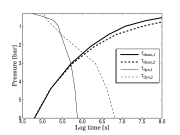
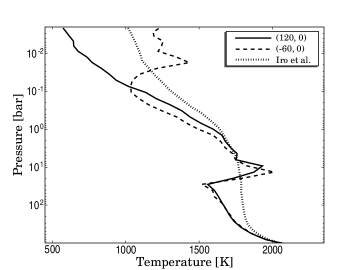
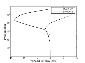
Figure 6.— Demonstrates quenching according to the eddy diffusion model of Smith (1998) in the nominal simulation for two vertical columns of atmosphere. The top panel shows $\tau_{\rm chem}$ and $\tau_{\rm dyn}$ on two vertical columns: (1) ($\lambda=120\arcdeg,\phi=0\arcdeg$) (solid lines) and (2) ($\lambda=-60\arcdeg,\phi=0\arcdeg$) (dashed lines). The quench level for the first column is where the thick and thin solid lines cross. Likewise, the quench level at ($\lambda=-60\arcdeg,\phi=0\arcdeg$) is where the thick and thin dashed lines cross. The middle and bottom panes show the temperatures and vertical velocities used to calculate $\tau_{\rm dyn}$ in each region.

The simplest model of disequilibrium chemistry defines the quench level to be where the timescale for reactions equals the timescale for dynamical advection in the system: i.e., quenching occurs at $\rm\tau_{\rm chem}=\tau_{\rm dyn}$. The latter quantity, $\tau_{\rm dyn}$, represents the timescale for dynamical motions to advect material across regions of atmosphere differing appreciably in temperature and pressure. Depending on local gradients in temperature, these timescales can be either large or small.

These considerations led Smith (1998) to revise the eddy diffusion model of quenching originally proposed by Prinn & Barshay (1977). In Smith (1998)’s model, the dynamical timescale is determined by eddy diffusion:

$$\tau_{\rm dyn}=\frac{L}{w},$$ (23)

where $L$ is a length scale and $w$ is the vertical velocity near the quench level.

Previous researchers estimated the quench level on Jupiter assuming $L=H$, where $H$ is the pressure scale height of the atmosphere. Smith (1998) demonstrates that the assumption of $L=H$ is incorrect for most planetary atmospheres. However, the eddy diffusion calculation is approximately correct if $L$ is replaced with an effective length scale $L_{\rm eff}$, “which depends on the e-folding length scales of $\tau_{\rm chem}$ and $\tau_{\rm dyn}$ and the pressure dependence of the equilibrium value of the chemical abundance.” He goes on to develop a recipe for determining $L_{\rm eff}$.

We apply the Smith (1998) recipe, which offers excellent insight into the chemistry governing our simulations, to the nominal atmosphere model. We also assume for the moment that quenching occurs in the vertical direction, not horizontally. The crucial quantity needed to estimate eddy diffusion is the vertical velocity (in height coordinates). Given $\omega=Dp/Dt$, the vertical velocity in height coordinates is approximately given by

$$w=\omega/(-\rho g),$$ (24)

where $\rho$ is the density and $g$ is the acceleration of gravity. It should be noted that this is not exact but is an excellent approximation for shallow atmospheres (Holton, 1992, p. 77–80).

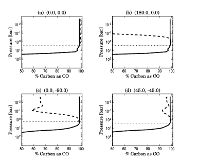
Figure 7.— Comparison of actual (solid line) and equilibrium (dashed line) CO abundance in the nominal simulation. Plotted is the % of carbon as CO—as opposed to $\rm CH_{4}$. Titles above the panels give the longitude and latitude for each column. The horizontal dotted lines show the quench level for each column as predicted with the Smith (1998) recipe.

To estimate quenching, it is essential to determine the appropriate length scale $L_{\rm eff}$ to use in computing $\tau_{\rm dyn}$, the timescale for eddy diffusion. Following the Smith (1998) recipe, $L_{\rm eff}\approx 0.5\;H$ in the first region, and $L_{\rm eff}\approx 0.3\;H$ second region. These are closer to $H$ than are appropriate for Jupiter because the equilibrium abundance of CO is uniformly high at the equator for $p>200$ mbar. This correction nonetheless causes a significant shift in the pressure at which quenching occurs in each case.

We show the quench levels (using $\tau_{\rm dyn}$ = $L_{\rm eff}/w$, not $H/w$) for both profiles in the top panel of Figure 6. The quench level near ($\lambda=120\arcdeg,\phi=0\arcdeg$) is about 3.0 bars; near ($\lambda=-60\arcdeg,\phi=0\arcdeg$), it is at 2.5 bar. The middle and bottom panels of Figure 6 show the vertical velocities and temperatures in these two regions. Here, we have averaged columns of $w$ over a $45\arcdeg$ angular radius on the sphere, which removes small-scale variations but preserves the large-scale structure of the vertical wind. For $p<1$ bar, downwelling occurs in the first region, whereas the second region, which is centered on the opposite hemisphere, has upwelling.

The Smith (1998) quenching model also predicts a homogeneous distribution of CO above the quench level, with the value determined by the equilibrium CO abundance at the quench level. Since this is high in both cases, the eddy diffusion model also predicts very little $\rm CH_{4}$ at the photosphere of HD 209458b. To emphasize the agreement between the Smith (1998) view of quenching and the actual abundance of CO in our simulations, we compare the equilibrium view to the CO abundance predicted in our simulation in Figure 7. This has been done on four columns of atmosphere to show the variation in quenching in different atmospheric regions. The Smith (1998) quench level in each pane is indicated by a thin dotted line, which agrees well with the convergence of the equilibrium vs. disequilibrium profiles (thick dashed and solid lines, respectively).

We conclude this discussion by reiterating why horizontal quenching near the day-night terminator is not of great importance in the simulation. Using reasoning analogous to our discussion above, the horizontal mixing timescale should be $\tau_{\rm dyn,\,h}=L_{\rm h}/u$, where $u$ is the supersonic zonal wind and $L_{\rm h}$ is a length scale appropriate for horizontal quenching. Lacking better information, $L_{\rm h}=2\pi R_{\rm p}$ (just the circumference of the planet). Note that the true value of the horizontal mixing time may be smaller than $2\pi R_{\rm p}/u$ in regions where parcels travel through large temperature gradients. But given the extremely fast wind speeds ($u\sim\!3000\;\rm m\;s^{-1}$) predicted in the upper layers, $\tau_{\rm dyn,\,h}$ can never be larger than this value. Assuming for the moment that this is correct, we obtain $\rm\tau_{dyn,\,h}\sim\!2\times 10^{5}\;s$. But Figure 6 clearly shows that $\tau_{\rm chem}\gg\rm 10^{5}\;s$ for $p<3$ bar, where vertical quenching is achieved. Hence, the quench level in the vertical has already been reached at levels where $\tau_{\rm chem}<\tau_{\rm dyn,\,h}$.

7. Discussion

7.1. Role of Photochemistry

Liang et al. (2004) show that the distribution of photochemical products, including aerosols and radicals, is insignificant at the pressure levels considered here compared to the primary constituents ($\rm H_{2}$, He, $\rm H_{2}O$, CO, and possibly $\rm CH_{4}$). But the effects of these species on the $\rm CO/CH_{4}$ reactions has not been explored here. Conceivably, OH and H coming from the photolysis of $\rm H_{2}O$ (Liang et al., 2003) could influence the reaction rates of the Yung et al. (1988) sequence.

We have not explored the consequences of photochemically enhanced OH and H populations on the $\rm CO/CH_{4}$ interconversion chemistry here. This effect is most likely to be noticeable in the highest layers of the model ($p$ ¡ 10 mbar), above which the stellar ultra-violet (UV) light is absorbed. In order to have an important effect on our predictions for the CO distribution, however, the chemical interconversion timescale resulting from interaction with photochemical radicals would have to be reduced to $\tau_{\rm chem}=10^{6}\;\rm s$ (or less). Such timescales would be very short compared with the values listed in Table 2 at these temperatures and pressures. That is, unless the photochemical production of radicals dominates the chemistry, the disequilibrium distributions will be substantially similar to those presented here.

7.2. Treatment of Radiation

Asynchronous rotation on hot Jupiters is possible, either due to eccentricity/obliquity pumping by other planets in the system or thermal tides (Showman & Guillot, 2002). In the case of HD 209458b, we expect synchronous rotation to hold more closely than planets in eccentric orbits. An asynchronous component to the rotation, due to thermal tides and transfer of angular momentum from the atmosphere to the interior, could conceivably influence the atmospheric dynamics solution (Figure 3). For example, our time-steady flow scenario might be superposed in some regions by a slow periodicity resulting from a radiative heating profile that slowly advances along the meridians. But as we discuss in §6, quenching is in the vertical. Adding asynchronous rotation to the model might change the details of the wind and temperature patterns but not the mean vertical velocity. Hence, the $\rm CO/CH_{4}$ distributions should not be sensitive to this correction.

Newtonian heating ignores potentially subtle feedbacks in the radiation physics. It has been used successfully, however, to model essential features of Earth’s general circulation (Holton, 1992, p. 409–411). We note that the approximation is likely to be less valid deep in the atmosphere of EGPs than it is for Earth. This is due to long radiative time constants and huge departures from radiative equilibrium. Hence, the use of Newtonian heating is probably the major source of error in our atmosphere model. We use it here partly because the approximation is reasonably valid for $p<2$ bar, where $\tau_{\rm rad}$ is less than several days. The scheme is also relatively easy to implement and performs well computationally, which is very desirable, as the AGDC2 itself demands considerable computational resources. We are able, therefore, to test the sensitivity of the results to a broad set of input parameters.

We note also that the abundances of $\rm H_{2}O$, CO, and $\rm CH_{4}$—used by Iro et al. (2005) to derive the contributions of these molecules to the total opacity—are calculated based on chemical equilibrium models. We demonstrate here, however, that chemical equilibrium does not hold for $p\ll 10$ bars. This internal inconsistency is inherent in our use of Newtonian cooling and is unfortunately unavoidable. Radiative-equilibrium models of HD 209458b’s atmosphere to date have all assumed chemical equilibrium. Even in the future, this coupling between dynamics and radiation will be difficult to disentangle because, as has been previously discussed, disequilibrium abundances depend on the overall meteorology.

Iro et al. (2005) also do not consider clouds. Where present, high silicate clouds could dominate the opacity and greatly perturb the atmospheric profile. Cloud deck optical thickness in general varies with wavelength, depending on the vertical extent of the cloud and the condensate particle sizes (Ackerman & Marley, 2001; Cooper et al., 2003). It is unclear what properties a silicate cloud high in the atmosphere would have. This is a complicated subject involving intricate feedbacks between radiation, cloud microphysics, and dynamics. We neglect the possibly crucial effects of clouds here. Including condensation processes will be a major future advance in the field of EGP atmosphere modeling.

7.3. Initial Conditions

Given the large $\tau_{\rm chem}$ values at low pressures, it is reasonable to wonder whether our solutions for the CO distribution depend on the initial conditions. For the simulations shown, we have assumed that CO is initially in chemical equilibrium everywhere (equation 5). As discussed in Cooper & Showman (2005), temperatures and winds are not strongly sensitive to the initial conditions. The primary concern here is whether vertical transport can mix CO upward rapidly enough to bring the CO mole fraction at the photosphere up to its value at the quench level.

Clearly, chemical processes occurring on timescales longer than $\sim\!1$ year cannot have run to completion by 1000 days of integration time. But we can argue on simple grounds that 1000 days is still long enough to determine $X_{\rm CO}$, even where $\tau_{\rm chem}\gg 1$ year. Assuming the vertical wind at 1 bar is $\sim\!10\rm\;m\;s^{-1}$, as shown by the model, and the vertical depth from the photosphere (100 mbar) to the quench level (3 bar) is $\sim\!2$% of the planetary radius (several scale heights), we would expect upward mixing to occur on timescales of $\sim\!1$ week. Thus, after $\sim\!1000$ days of integration time, the CO concentration should approach the value at the quench level.

We have run two additional simulations with different initial conditions. The first simulation assumes no initial CO in the atmosphere; i.e., 100% of the carbon is $\rm CH_{4}$. The second simulation assumes no initial $\rm CH_{4}$; i.e., 100% of the carbon is CO. Both use the input parameters of the nominal model in all other respects. Therefore, temperatures and winds are the same as in the nominal case. After even several hundred days of simulation time, the solutions for CO in these two cases are virtually indistinguishable from the nominal simulation (see Figure 5). These tests demonstrate that memory of the initial condition for $X_{\rm CO}$ has been erased by $t_{\rm sim}=1000$ days.

7.4. Metallicity and C/O

Our nominal simulation assumes solar abundances based on the Lodders & Fegley (1998) compilation. We note that the precise values of the solar abundances, especially C, N, and O, have undergone minor modifications in the past seven years, some of which are still under discussion within the scientific community (Grevesse & Sauval, 1998; Mahaffy et al., 2000; Allende Prieto et al., 2001, 2002; Lodders, 2003; Asplund et al., 2006). In particular, the CNO abundances, along with those of the noble gases, have been revised down from the geochemically based abundances of Anders & Grevesse (1989); Lodders & Fegley (1998). The C/O ratio is now thought to be exactly 0.5; following Lodders & Fegley (1998), we use C/O = 0.57 here. Incorporating these updates to the solar abundances will modify the results presented here somewhat, though the correction is likely to be fairly minor.

From stellar spectroscopy, the endowment of heavy elements in the star HD 209458 is well-known to be about solar: $\rm[Fe/H]=0.014\pm 0.03$ (Fischer & Valenti, 2005). That says nothing about the metallicity of the planet orbiting it, which has not yet been measured. Jupiter and Saturn boast pronounced enrichments in heavy elements relative to the Sun, suggesting EGPs may also be metal-rich compared to their host stars. We consider here the effects of increasing the relative proportions of carbon and oxygen in HD 209458b’s atmosphere.

Suppose the constants $c_{1}$ and $c_{2}$ in equations 1 and 2 are both increased by a factor of 10. This is a much greater metal abundance than is seen on Jupiter, which has enrichment of carbon and nitrogen by a factor of $\sim\!3$ relative to the Sun (from Galileo probe measurements; the probe was not successful in measuring the abundance of oxygen—see Wong et al., 2004). As carbon and oxygen in this case are still minor constituents, this change will not appreciably affect the mean molecular weight or heat capacity of the atmosphere. According to our chemical equilibrium solution, equation 5, increased [Fe/H] favors the formation of CO. That is, for a given temperature and pressure, the ratio $X_{\rm CO}/X_{\rm CH_{4}}$ is higher for [Fe/H] = +1.0 than it is at [Fe/H] = 0.0, in agreement with Lodders & Fegley (2002). This implies that, relative to the solar metallicity case, the quench level should have a greater abundance of CO in the [Fe/H] = +1.0 atmosphere by more than a factor of 10. Hence, we would also expect the photosphere to show highly abundant CO.

We have run a high-metallicity simulation, in which we set [Fe/H] = 1.0 in the atmosphere. The other parameters of this model are identical to the nominal simulation, so the dynamics are the same. We indeed see in this simulation that 100% of the carbon atoms are in CO, with no $\rm CH_{4}$ at all (as opposed to 1–2% $\rm CH_{4}$ predicted in the nominal case).

We stress that the above discussion assumes atmospheric temperatures do not change drastically as a result of increasing the metallicity. This assumption may not be correct for all EGPs. We note, however, that Fortney et al. (2005) consider metallicity adjustments to their radiative-equilibrium models of HD 209458b and TrES-1. They find that the effective temperature of TrES-1 increases by only $\sim\!14\;\rm K$ for a metallicity of $5\times$ solar. The direction of the effect—warming, not cooling—also favors the appearance of CO.

Similarly, increasing the C/O ratio in the atmosphere will not inhibit CO’s formation at the temperature of HD 209458b’s atmosphere. In the Sun, $\rm C/O\approx 0.5$. If $\rm C/O\gtrsim 1$, CO can potentially take up 100% of the available oxygen, in which case $\rm H_{2}O$ will be depleted. Atmospheres showing the spectral signatures of CO without prominent $\rm H_{2}O$ features very likely have a high C/O ratio relative to solar. The effects of super-solar abundances and enhanced C/O are discussed in more detail elsewhere (Fortney et al., 2005; Seager et al., 2005).

8. Conclusions / Implications

We have run 3D numerical simulations of HD 2094548b’s atmosphere to explore the chemistry of carbon. We advect CO through the atmosphere as a passive tracer, relaxing its concentration toward the local chemical equilibrium value. The relaxation timescale depends on the reaction pathways that convert CO to $\rm CH_{4}$. We follow recent previous work on disequilibrium carbon chemistry (Griffith & Yelle, 1999; Bézard et al., 2002) and assume that the Yung et al. (1988) sequence is the most efficient mechanism for the chemical reduction of CO.

We calculate the relative abundances of CO, $\rm CH_{4}$, and $\rm H_{2}O$, which are the main species of carbon and oxygen in the atmosphere. Our nominal simulation models HD 209458b specifically. For comparison, we have also run simulations of “cold” and “hot” atmospheres. The cold simulation is representative of a planet that is $\sim\!300$ K cooler than HD 209458b; the hot simulation models a planet $\sim\!300$ K warmer.

The atmospheric dynamics by 1000 Earth days of simulation time has reached the steady state described in Cooper & Showman (2005). Eastward winds in the nominal model reach $\rm\sim\!4000\;m\;s^{-1}$ at the photosphere, with corresponding temperature contrasts of $\rm\sim\!500\;K$. Atmospheric dynamics partially redistribute the thermal energy to the planet’s nightside, but longitudinal contrasts in temperature are apparent down to $\sim\!2$ bars.

Chemical equilibrium has been the basis of all prior discussions about CO and $\rm CH_{4}$ on HD 209458b. We show here, though, that the equilibrium picture of $\rm CO/CH_{4}$ chemistry is a vast misconception. In regions where chemical equilibrium does not hold, the true CO abundance depends not only on local quantities but also on the overall meteorology.

We show that the timescale for $\rm CO/CH_{4}$ interconversion depends sensitively on both temperature and pressure (Table 2). At low temperatures and pressures, reactions are slow; at high temperatures and pressures, reactions are fast. As a result of long reaction times, CO is not expected to be in chemical equilibrium in the 1–1000 mbar region (the “visible” layers). Chemical equilibrium in the model atmosphere is attained deeper in the atmosphere ($p\gtrsim 5$ bars), where the interconversion timescale is short relative to dynamical mixing times.

The atmosphere is well-mixed by vertical motions, which leads to vertical (as opposed to horizontal) quenching. Vertical quenching results in photospheric CO concentrations exceeding chemical equilibrium values by many orders of magnitude. The simulations show that CO, $\rm CH_{4}$, and $\rm H_{2}O$ will be homogeneously distributed throughout the photosphere of HD 209458b and similar planets. At $p\lesssim 2$ bars, almost all of the carbon is in the form of CO, even in cold regions such as the nightside. Consequently, we expect water vapor to be less plentiful than previously thought. These conclusions are consistent with the simpler view of quenching presented by Smith (1998).

The metallicity of HD 209458b is not known. Our nominal simulation assumes solar abundances. We have also run a variation on the nominal model that assumes ten times enhancement of the heavy elements: [Fe/H] = +1.0. Disequilibrium effects operate similarly in this model, and the ratio of CO to total carbon in the atmosphere remains close to 100%. Indeed, higher metallicity favors the formation of CO over $\rm CH_{4}$. Hence, if close-in EGPs have characteristically super-solar abundances, CO could be prominent at the photospheres of planets even cooler than $\rm T_{eff}=1000\;K$.

Likewise, increasing the C/O ratio would not significantly inhibit CO’s formation at depth (and subsequent transport up to the photosphere). If C/O exceeds the solar value of 0.5 in the Sun, CO on HD 209458b should be highly abundant. The tell-tale sign of this scenario at HD 209458b’s effective temperature is $\rm H_{2}O$ depletion.

Our results have several interesting consequences for near-future observations of close-in EGPs, although a thorough analysis of close-in EGP spectra is beyond the scope of this work. We conclude simply with a brief description of the implications of these findings.

The hot model shows that planets significantly warmer than HD 209458b should have no $\rm CH_{4}$ in their photospheres, unless the C/O ratio is greater than 1. But in planets significantly cooler than HD 209458b, disequilibrium effects should raise the concentration of CO to detectable levels. The specific value of $X_{\rm CO}$ cannot be predicted with definite precision based on these simulations; there are too many uncertainties in the model’s inputs. However, examination of the values of $\tau_{\rm chem}$ (Table 2) suggests that 1–10 bar may be the approximate quench level for all close-in EGPs within $\rm 750\;K$ of HD 209458b’s effective temperature ($\rm T_{eff}\sim\!1350$ K for this planet). The relative concentrations of CO and $\rm CH_{4}$ at the photosphere are therefore diagnostic of local conditions in the 1–10 bar region of the atmosphere, which is deeper than observations can directly probe. Neither species has yet been detected in this planet’s atmosphere (Richardson et al., 2003b, a; Deming et al., 2005a). Our results here suggest that $\rm CH_{4}$ depletion (not depletion of CO) is the more likely situation; even in chemical equilibrium, $\rm CH_{4}$ is likely to be depleted at the limb.

Measurements of carbon-bearing species can thus serve as a useful calibration tool of radiation and dynamics models of these planets. It should be noted that metallicity also plays a role in determining the abundance of CO at the quench level. This may be a difficult effect to deconvolve from temperature and pressure, unless absolute concentrations can be measured. For near-future explorations, what is crucial here is that planets with little or no $\rm CH_{4}$ must be very much warmer than TrES-1 or else cooler, but very metal-rich (as high metallicity favors the formation of CO over $\rm CH_{4}$).

It is known that HD 209458b does contain carbon and oxygen (Vidal-Madjar et al., 2004). As Deming et al. (2005a) discuss, the null detection of CO using NIRSPEC on Keck II cannot be easily attributed to CO depletion in HD 209458b’s atmosphere. This lends credence to the hypothesis of a high cloud or haze obscuring the spectral features of CO near 2 $\micron$. As discussed by Fortney (2005), however, the slant geometry implies that even a layer of modest optical thickness could hide the signature of CO. It may be possible to distinguish between these and other scenarios.

Our results suggest that TrES-1, which orbits a K-type star, should also show strong CO absorption features in its spectrum. A high silicate condensation cloud obscuring the photosphere is not expected on TrES-1 due to lower temperatures overall. The condensation of silicates should occur at much greater depth in TrES-1’s atmosphere. It would be very illuminating to perform a transmission spectroscopy search for CO on TrES-1. Discovery of CO on TrES-1 would make a strong case for high silicate clouds in the atmosphere of HD 209458b. If CO is also not detectable on TrES-1 by transmission spectroscopy, on the other hand, the hypothesis of stratospheric haze (that hides CO on both planets) becomes more appealing.

The ubiquitousness of CO throughout the photospheres of close-in EGPs should also have profound implications for the spectra of these objects. Our results for the cold model suggest that CO may even be abundant on cooler EGPs than TrES-1. If so, CO’s spectral signature should be detectable. The absorption features of $\rm H_{2}O$ may also be less pronounced, especially on hot planets, in which over half of the available oxygen atoms are bound up in CO. In addition to the 2 $\micron$ band pass explored by Deming et al. (2005a), we suggest searches for CO in the rovibrational fundamental near 4.5 $\rm micron$. If present, the opacity of CO overwhelms that of $\rm H_{2}O$ vapor at this wavelength, even more so than the wavelength region explored in Deming et al. (2005a). As an IR window also exists at 4.5 $\micron$, this observation may also be possible using ground-based platforms.

It is noteworthy also that these simulations predict a homogeneous distribution of CO, $\rm CH_{4}$, and $\rm H_{2}O$ in HD 209458b’s atmosphere, although the temperature is almost certainly not isothermal at the photosphere. Cooper & Showman (2005) show that temperature variations over the photosphere can lead to brightness variations in the planet with orbital phase. It must be emphasized that the synthetic light curve of Cooper & Showman (2005) pertained to the bolometric luminosity of the planet (i.e., the emission integrated over all wavelengths); nothing is directly implied about the planet’s brightness at a particular wavelength. The flux contrast of the planet’s photosphere over a full orbital period would likely be suppressed somewhat by a homogeneous distribution of CO and $\rm CH_{4}$, as the distribution of these species determines the level of the photosphere [J. Fortney, private communication]. Wavelength-dependent light curves will require generating synthetic spectra using a radiative transfer model, a task we leave for future work. But we hope this discussion will inspire near-future searches for CO and $\rm CH_{4}$ on these planets, some of which should be possible even with ground-based telescopes.

Table 1CO in Chemical Equilibrium

T [K]	10 mbar	100 mbar	500 mbar	1 bar	5 bar	10 bar	100 bar	500 bar	1 kbar
500	$1.7\times 10^{-9}$	0.0	0.0	0.0	0.0	0.0	0.0	0.0	0.0
750	$5.5\times 10^{-2}$	$6.0\times 10^{-4}$	$2.4\times 10^{-5}$	$6.0\times 10^{-6}$	$2.4\times 10^{-7}$	$6.0\times 10^{-8}$	$6.3\times 10^{-10}$	0.0	0.0
1000	1.0	0.73	0.15	$4.4\times 10^{-2}$	$1.9\times 10^{-3}$	$4.6\times 10^{-4}$	$4.7\times 10^{-6}$	$1.9\times 10^{-7}$	$4.7\times 10^{-8}$
1250	1.0	1.0	0.95	0.85	0.27	$9.4\times 10^{-2}$	$1.1\times 10^{-3}$	$4.4\times 10^{-5}$	$1.1\times 10^{-5}$
1500	1.0	1.0	1.0	0.99	0.89	0.71	$4.0\times 10^{-2}$	$1.7\times 10^{-3}$	$4.2\times 10^{-4}$
1750	1.0	1.0	1.0	1.0	0.99	0.96	0.32	$2.2\times 10^{-2}$	$5.7\times 10^{-3}$
2000	1.0	1.0	1.0	1.0	1.0	0.99	0.70	0.13	$3.7\times 10^{-2}$
2500	1.0	1.0	1.0	1.0	1.0	1.0	0.96	0.61	0.32

Note. — Fraction of carbon in the atmosphere present as CO (i.e., the ratio $X_{\rm CO}\,/\,c_{1}$), assuming chemical equilibrium (see eq. 1 – 5). We obtain these values by solving equation 5, which calculates the chemical equilibrium of CO in a gas of solar composition. Our treatment follows Lodders & Fegley (2002). Data for the standard Gibbs free energies of formation for CO, $\rm CH_{4}$, and $\rm H_{2}O$ are taken from the NIST-JANAF tabulations (Chase, 1998).

Table 2 CO/$\rm CH_{4}$ interconversion timescale

T [K]	10 mbar	100 mbar	500 mbar	1 bar	5 bar	10 bar	100 bar	500 bar	1 kbar
500	$1.0\times 10^{24}$	$4.3\times 10^{21}$	$1.7\times 10^{20}$	$4.9\times 10^{19}$	$3.7\times 10^{18}$	$1.3\times 10^{18}$	$4.0\times 10^{16}$	$3.5\times 10^{15}$	$1.3\times 10^{15}$
750	$9.0\times 10^{17}$	$2.8\times 10^{15}$	$5.2\times 10^{13}$	$9.3\times 10^{12}$	$1.9\times 10^{11}$	$3.9\times 10^{10}$	$4.2\times 10^{8}$	$3.1\times 10^{7}$	$1.1\times 10^{7}$
1000	$1.1\times 10^{15}$	$3.6\times 10^{12}$	$6.4\times 10^{10}$	$1.1\times 10^{10}$	$2.1\times 10^{8}$	$3.7\times 10^{7}$	$1.4\times 10^{5}$	$4.8\times 10^{3}$	$1.3\times 10^{3}$
1250	$2.3\times 10^{13}$	$7.4\times 10^{10}$	$1.3\times 10^{9}$	$2.3\times 10^{8}$	$4.2\times 10^{6}$	$7.4\times 10^{5}$	$2.4\times 10^{3}$	52	11
1500	$1.9\times 10^{12}$	$6.0\times 10^{9}$	$1.1\times 10^{8}$	$1.9\times 10^{7}$	$3.4\times 10^{5}$	$6.0\times 10^{4}$	$1.9\times 10^{2}$	3.6	0.68
1750	$3.3\times 10^{11}$	$1.0\times 10^{9}$	$1.9\times 10^{7}$	$3.3\times 10^{6}$	$5.9\times 10^{4}$	$1.0\times 10^{4}$	33	$0.60$	$0.11$
2000	$9.1\times 10^{10}$	$2.9\times 10^{8}$	$5.1\times 10^{6}$	$9.1\times 10^{5}$	$1.6\times 10^{4}$	$2.9\times 10^{3}$	9.1	0.16	$2.9\times 10^{-2}$
2500	$1.6\times 10^{10}$	$5.0\times 10^{7}$	$8.9\times 10^{5}$	$1.6\times 10^{5}$	$2.8\times 10^{3}$	$5.0\times 10^{2}$	1.6	$2.8\times 10^{-2}$	$5.0\times 10^{-3}$

Note. — Timescale in seconds for CO/$\rm CH_{4}$ interconversion in the Yung et al. (1988) catalyzed reaction sequence at the same temperatures and pressures used in Table 1. These values have been computed using equations 19 and 18, following equations (7) and (8) of Bézard et al. (2002). The expression for $\rm\tau_{chem}$ derives from consideration of the rate of the reverse of reaction 9, which has been measured in the laboratory (Page et al., 1989).

References

- Ackerman & Marley (2001) Ackerman, A. S., & Marley, M. S. 2001, ApJ, 556, 872
- Allende Prieto et al. (2001) Allende Prieto, C., Lambert, D. L., & Asplund, M. 2001, ApJ, 556, L63
- Allende Prieto et al. (2002) —. 2002, ApJ, 573, L137
- Alonso et al. (2004) Alonso, R., Brown, T. M., Torres, G., Latham, D. W., Sozzetti, A., Mandushev, G., Belmonte, J. A., Charbonneau, D., Deeg, H. J., Dunham, E. W., O’Donovan, F. T., & Stefanik, R. P. 2004, ApJ, 613, L153
- Anders & Grevesse (1989) Anders, E., & Grevesse, N. 1989, Geochim. Cosmochim. Acta, 53, 197
- Arakawa & Lamb (1977) Arakawa, A., & Lamb, V. 1977, Methods in Computational Physics, 17, 173
- Asplund et al. (2006) Asplund, M., Grevesse, N., & Sauval, A. J. 2006, Communications in Asteroseismology, 147, 76
- Atreya et al. (1999) Atreya, S. K., Wong, M. H., Owen, T. C., Mahaffy, P. R., Niemann, H. B., de Pater, I., Drossart, P., & Encrenaz, T. 1999, Planet. Space Sci., 47, 1243
- Barman et al. (2005) Barman, T. S., Hauschildt, P. H., & Allard, F. 2005, ApJ, 632, 1132
- Barman et al. (2002) Barman, T. S., Hauschildt, P. H., Schweitzer, A., Stancil, P. C., Baron, E., & Allard, F. 2002, ApJ, 569, L51
- Barnes & Fortney (2003) Barnes, J. W., & Fortney, J. J. 2003, ApJ, 588, 545
- Beer (1975) Beer, R. 1975, ApJ, 200, L167
- Bézard et al. (2002) Bézard, B., Lellouch, E., Strobel, D., Maillard, J.-P., & Drossart, P. 2002, Icarus, 159, 95
- Bouchy et al. (2005a) Bouchy, F., Pont, F., Melo, C., Santos, N. C., Mayor, M., Queloz, D., & Udry, S. 2005a, A&A, 431, 1105
- Bouchy et al. (2004) Bouchy, F., Pont, F., Santos, N. C., Melo, C., Mayor, M., Queloz, D., & Udry, S. 2004, A&A, 421, L13
- Bouchy et al. (2005b) Bouchy, F., Udry, S., Mayor, M., Moutou, C., Pont, F., Iribarne, N., da Silva, R., Ilovaisky, S., Queloz, D., Santos, N. C., Ségransan, D., & Zucker, S. 2005b, A&A, 444, L15
- Brown (2001) Brown, T. M. 2001, ApJ, 553, 1006
- Brown et al. (2001) Brown, T. M., Charbonneau, D., Gilliland, R. L., Noyes, R. W., & Burrows, A. 2001, ApJ, 552, 699
- Burkert et al. (2005) Burkert, A., Lin, D. N. C., Bodenheimer, P. H., Jones, C. A., & Yorke, H. W. 2005, ApJ, 618, 512
- Burrows et al. (2004) Burrows, A., Hubeny, I., Hubbard, W. B., Sudarsky, D., & Fortney, J. J. 2004, ApJ, 610, L53
- Burrows et al. (2005) Burrows, A., Hubeny, I., & Sudarsky, D. 2005, ApJ, 625, L135
- Burrows & Sharp (1999) Burrows, A., & Sharp, C. M. 1999, ApJ, 512, 843
- Burrows et al. (2003) Burrows, A., Sudarsky, D., & Hubbard, W. B. 2003, ApJ, 594, 545
- Chabrier et al. (2004) Chabrier, G., Barman, T., Baraffe, I., Allard, F., & Hauschildt, P. H. 2004, ApJ, 603, L53
- Chamberlain & Hunten (1987) Chamberlain, J. W., & Hunten, D. M. 1987, Orlando FL Academic Press Inc International Geophysics Series, 36
- Charbonneau et al. (2005) Charbonneau, D., Allen, L. E., Megeath, S. T., Torres, G., Alonso, R., Brown, T. M., Gilliland, R. L., Latham, D. W., Mandushev, G., O’Donovan, F. T., & Sozzetti, A. 2005, ApJ, 626, 523
- Charbonneau et al. (2000) Charbonneau, D., Brown, T. M., Latham, D. W., & Mayor, M. 2000, ApJ, 529, L45
- Charbonneau et al. (2002) Charbonneau, D., Brown, T. M., Noyes, R. W., & Gilliland, R. L. 2002, ApJ, 568, 377
- Chase (1998) Chase, M. W., J. 1998, Journal of Physical and Chemical Reference Data, Monograph 9
- Cho et al. (2003) Cho, J. Y.-K., Menou, K., Hansen, B. M. S., & Seager, S. 2003, ApJ, 587, L117
- Cooper & Showman (2005) Cooper, C. S., & Showman, A. P. 2005, ApJ, 629, L45
- Cooper et al. (2003) Cooper, C. S., Sudarsky, D., Milsom, J. A., Lunine, J. I., & Burrows, A. 2003, ApJ, 586, 1320
- Correia & Laskar (2001) Correia, A. C. M., & Laskar, J. 2001, Nature, 411, 767
- Deming et al. (2005a) Deming, D., Brown, T. M., Charbonneau, D., Harrington, J., & Richardson, L. J. 2005a, ApJ, 622, 1149
- Deming et al. (2005b) Deming, D., Seager, S., Richardson, L. J., & Harrington, J. 2005b, Nature, 434, 740
- Dowling et al. (1998) Dowling, T. E., Fischer, A. S., Gierasch, P. J., Harrington, J., Lebeau, R. P., & Santori, C. M. 1998, Icarus, 132, 221
- Fegley & Lodders (1996) Fegley, B. J., & Lodders, K. 1996, ApJ, 472, L37+
- Fischer & Valenti (2005) Fischer, D. A., & Valenti, J. 2005, ApJ, 622, 1102
- Fortney (2005) Fortney, J. J. 2005, MNRAS, 910
- Fortney et al. (2005) Fortney, J. J., Marley, M. S., Lodders, K., Saumon, D., & Freedman, R. 2005, ApJ, 627, L69
- Fortney et al. (2003) Fortney, J. J., Sudarsky, D., Hubeny, I., Cooper, C. S., Hubbard, W. B., Burrows, A., & Lunine, J. I. 2003, ApJ, 589, 615
- Goukenleuque et al. (2000) Goukenleuque, C., Bézard, B., Joguet, B., Lellouch, E., & Freedman, R. 2000, Icarus, 143, 308
- Grevesse & Sauval (1998) Grevesse, N., & Sauval, A. J. 1998, Space Science Reviews, 85, 161
- Griffith & Yelle (1999) Griffith, C. A., & Yelle, R. V. 1999, ApJ, 519, L85
- Guillot et al. (1996) Guillot, T., Burrows, A., Hubbard, W. B., Lunine, J. I., & Saumon, D. 1996, ApJ, 459, L35+
- Henry et al. (2000) Henry, G. W., Marcy, G. W., Butler, R. P., & Vogt, S. S. 2000, ApJ, 529, L41
- Holton (1992) Holton, J. R. 1992, An introduction to dynamic meteorology (International geophysics series, San Diego, New York: Academic Press, —c1992, 3rd ed.)
- Iro et al. (2005) Iro, N., Bézard, B., & Guillot, T. 2005, A&A, 436, 719
- Kalnay (2003) Kalnay, E. 2003, Atmospheric modeling, data assimilation and predictability (Cambridge: Cambridge University Press, 2003)
- Konacki et al. (2003) Konacki, M., Torres, G., Jha, S., & Sasselov, D. D. 2003, Nature, 421, 507
- Konacki et al. (2005) Konacki, M., Torres, G., Sasselov, D. D., & Jha, S. 2005, ApJ, 624, 372
- Larson et al. (1978) Larson, H. P., Fink, U., & Treffers, R. C. 1978, ApJ, 219, 1084
- Laughlin et al. (2005a) Laughlin, G., Marcy, G. W., Vogt, S. S., Fischer, D. A., & Butler, R. P. 2005a, ApJ, 629, L121
- Laughlin et al. (2005b) Laughlin, G., Wolf, A., Vanmunster, T., Bodenheimer, P., Fischer, D., Marcy, G., Butler, P., & Vogt, S. 2005b, ApJ, 621, 1072
- Liang et al. (2003) Liang, M.-C., Parkinson, C. D., Lee, A. Y.-T., Yung, Y. L., & Seager, S. 2003, ApJ, 596, L247
- Liang et al. (2004) Liang, M.-C., Seager, S., Parkinson, C. D., Lee, A. Y.-T., & Yung, Y. L. 2004, ApJ, 605, L61
- Lodders (2003) Lodders, K. 2003, ApJ, 591, 1220
- Lodders & Fegley (1998) Lodders, K., & Fegley, B. 1998, The planetary scientist’s companion / Katharina Lodders, Bruce Fegley. (The planetary scientist’s companion / Katharina Lodders, Bruce Fegley. New York : Oxford University Press, 1998. QB601 .L84 1998)
- Lodders & Fegley (2002) —. 2002, Icarus, 155, 393
- Mahaffy et al. (2000) Mahaffy, P. R., Niemann, H. B., Alpert, A., Atreya, S. K., Demick, J., Donahue, T. M., Harpold, D. N., & Owen, T. C. 2000, J. Geophys. Res., 105, 15061
- Moses (1992) Moses, J. I. 1992, Icarus, 99, 368
- Moses et al. (2000) Moses, J. I., Lellouch, E., Bézard, B., Gladstone, G. R., Feuchtgruber, H., & Allen, M. 2000, Icarus, 145, 166
- Noll et al. (1997) Noll, K. S., Geballe, T. R., & Marley, M. S. 1997, ApJ, 489, L87+
- Oppenheimer et al. (1998) Oppenheimer, B. R., Kulkarni, S. R., Matthews, K., & van Kerkwijk, M. H. 1998, ApJ, 502, 932
- Page et al. (1989) Page, M., Lin, M. C., He, Y., & Choudhury, T. 1989, J. Phys. Chem., 93, 4404
- Polvani et al. (2004) Polvani, L. M., Scott, R. K., & Thomas, S. J. 2004, Monthly Weather Review, 132, 2539
- Pont et al. (2004) Pont, F., Bouchy, F., Queloz, D., Santos, N. C., Melo, C., Mayor, M., & Udry, S. 2004, A&A, 426, L15
- Prather et al. (1978) Prather, M. J., Logan, J. A., & McElroy, M. B. 1978, ApJ, 223, 1072
- Press et al. (1992) Press, W. H., Teukolsky, S. A., Vetterling, W. T., & Flannery, B. P. 1992, Numerical recipes in C. The art of scientific computing (Cambridge: University Press, —c1992, 2nd ed.)
- Prinn & Barshay (1977) Prinn, R. G., & Barshay, S. S. 1977, Science, 198, 1031
- Richardson et al. (2003a) Richardson, L. J., Deming, D., & Seager, S. 2003a, ApJ, 597, 581
- Richardson et al. (2003b) Richardson, L. J., Deming, D., Wiedemann, G., Goukenleuque, C., Steyert, D., Harrington, J., & Esposito, L. W. 2003b, ApJ, 584, 1053
- Sato et al. (2005) Sato, B., Fischer, D. A., Henry, G. W., Laughlin, G., Butler, R. P., Marcy, G. W., Vogt, S. S., Bodenheimer, P., Ida, S., Toyota, E., Wolf, A., Valenti, J. A., Boyd, L. J., Johnson, J. A., Wright, J. T., Ammons, M., Robinson, S., Strader, J., McCarthy, C., Tah, K. L., & Minniti, D. 2005, ApJ, 633, 465
- Saumon et al. (2000) Saumon, D., Geballe, T. R., Leggett, S. K., Marley, M. S., Freedman, R. S., Lodders, K., Fegley, B., & Sengupta, S. K. 2000, ApJ, 541, 374
- Seager et al. (2005) Seager, S., Richardson, L. J., Hansen, B. M. S., Menou, K., Cho, J. Y.-K., & Deming, D. 2005, ApJ, 632, 1122
- Seager & Sasselov (1998) Seager, S., & Sasselov, D. D. 1998, ApJ, 502, L157+
- Showman & Guillot (2002) Showman, A. P., & Guillot, T. 2002, A&A, 385, 166
- Smith (1998) Smith, M. D. 1998, Icarus, 132, 176
- Suarez & Takacs (1995) Suarez, M. J., & Takacs, L. L., eds. 1995, Technical report series on global modeling and data assimilation. Volume 5: Documentation of the ARIES/GEOS dynamical core, version 2
- Sudarsky et al. (2003) Sudarsky, D., Burrows, A., & Hubeny, I. 2003, ApJ, 588, 1121
- Tsang & Hampson (1986) Tsang, W., & Hampson, R. F. 1986, Journal of Physical and Chemical Reference Data, 15, 1087
- Vidal-Madjar et al. (2004) Vidal-Madjar, A., Désert, J.-M., Lecavelier des Etangs, A., Hébrard, G., Ballester, G. E., Ehrenreich, D., Ferlet, R., McConnell, J. C., Mayor, M., & Parkinson, C. D. 2004, ApJ, 604, L69
- Vidal-Madjar et al. (2003) Vidal-Madjar, A., Lecavelier des Etangs, A., Désert, J.-M., Ballester, G. E., Ferlet, R., Hébrard, G., & Mayor, M. 2003, Nature, 422, 143
- Winn & Holman (2005) Winn, J. N., & Holman, M. J. 2005, ApJ, 628, L159
- Wong et al. (2004) Wong, M. H., Mahaffy, P. R., Atreya, S. K., Niemann, H. B., & Owen, T. C. 2004, Icarus, 171, 153
- Yung et al. (1988) Yung, Y. L., Drew, W. A., Pinto, J. P., & Friedl, R. R. 1988, Icarus, 73, 516