THE MASS-METALLICITY RELATION AT $z\gtrsim 2$

Abstract

We use a sample of 87 rest-frame ultraviolet-selected star-forming galaxies with mean spectroscopic redshift $\langle z\rangle=2.26\pm 0.17$ to study the correlation between metallicity and stellar mass at high redshift. Using stellar masses determined from spectral energy distribution fitting to $U_{n}G{\cal R}JK_{s}$ (and Spitzer IRAC, for 37% of the sample) photometry, we divide the sample into six bins in stellar mass, and construct six composite $\rm H\alpha$ + [N II] spectra from all of the objects in each bin. We estimate the mean oxygen abundance in each bin from the [N II]/$\rm H\alpha$ ratio, and find a monotonic increase in metallicity with increasing stellar mass, from $12+\rm log(O/H)<8.2$ for galaxies with $\langle M_{\star}\rangle=2.7\times 10^{9}$ $\rm M_{\odot}$ to $12+\rm log(O/H)=8.6$ for galaxies with $\langle M_{\star}\rangle=1.0\times 10^{11}$ $\rm M_{\odot}$. The mass-metallicity relation at $z\sim 2$ is offset from the local mass-metallicity relation by $\sim 0.3$ dex, in the sense that galaxies of a given stellar mass have lower metallicity at high redshift. A corresponding metallicity-luminosity relation constructed by binning the galaxies according to rest-frame $B$ magnitude shows no significant correlation. This lack of correlation is explained by the known large variation in the rest-frame optical mass-to-light ratio at $z\sim 2$, and indicates that the correlation with stellar mass is more fundamental. We use the empirical relation between star formation rate density and gas density to estimate the gas fractions of the galaxies, finding an increase in gas fraction with decreasing stellar mass. The median gas fraction is more than two times higher than that found in local star-forming galaxies, providing a natural explanation for the lower metallicities of the $z\sim 2$ galaxies. These gas fractions combined with the observed metallicities allow the estimation of the effective yield $y_{\rm eff}$ as a function of stellar mass; in contrast to observations in the local universe which show a decrease in $y_{\rm eff}$ with decreasing baryonic mass, we find a slight increase. Such a variation of metallicity with gas fraction is best fit by a model with supersolar yield and an outflow rate $\sim 4$ times higher than the star formation rate. We conclude that the mass-metallicity relation at high redshift is driven by the increase in metallicity as the gas fraction decreases through star formation, and is likely modulated by metal loss from strong outflows in galaxies of all masses. Our ability to detect differential metal loss as a function of mass is limited by the small range of baryonic masses spanned by the galaxies in the sample, but there is no evidence for preferential loss of metals from low mass galaxies as has been suggested in the local universe.

1. Introduction

Correlations between mass and metallicity or luminosity and metallicity are well-established in nearby galaxies, ranging over orders of magnitude in mass and luminosity and spanning $\sim 2$ dex in chemical abundance. Lequeux et al. (1979) first observed a correlation between heavy element abundance and the total mass of galaxies; since then, most investigations have focused on the metallicity-luminosity relationship (e.g. Skillman et al. 1989; Zaritsky et al. 1994; Garnett et al. 1997; Lamareille et al. 2004; Salzer et al. 2005, to name only a few), though others have studied correlations between metallicity and rotational velocity (Zaritsky et al. 1994; Garnett 2002). The relationship between metallicity and stellar mass has recently been quantified by Tremonti et al. (2004, T04 hereafter), using a sample of $\sim 53,000$ galaxies from the Sloan Digital Sky Survey (SDSS). Such correlations provide insight into the process of galaxy evolution, as they allow the study of the history of star formation and gas enrichment or depletion through current, observable properties. Chemical enrichment is a record of star formation history, modulated by inflows and outflows of gas, while the stellar mass provides a more straightforward measure of the accumulated conversion of gas into stars and thus of the metals returned to the gas as the byproducts of star formation.

It has long been recognized that a correlation between stellar mass and gas phase metallicity is a natural consequence of the conversion of gas into stars in a closed system (van den Bergh 1962; Schmidt 1963; Searle & Sargent 1972). The principal ingredients of this “simple” or “closed-box” model are the metallicity, the yield from star formation (defined as the mass of metals produced and ejected by star formation, in units of the mass that remains locked in long-lived stars and remnants), and the gas fraction. If there are no inflows or outflows of gas, the metallicity is a simple function of the yield and the gas fraction, and rises as the gas is converted into stars and enriched by star formation according to the yield. The model is subject to the further assumptions that the system is well-mixed at all times, that it begins as pure gas with primordial abundances, that stellar evolution and nucleosynthesis take place instantaneously compared to the timescale of galactic evolution (the instantaneous recycling approximation), and that the IMF and the yield in primary elements of stars of a given mass are constant. This simple model, in combination with the observation that lower mass galaxies tend to have higher gas fractions (McGaugh & de Blok 1997; Bell & de Jong 2000), results in a correlation between metallicity and total mass.

One of the first, best-known failures of the simple model is the so-called “G-dwarf problem”: the closed-box model overpredicts the number of low-metallicity stars observed in the solar neighborhood. This is one aspect of the more fundamental problem that galaxies are clearly not closed boxes. On the one hand, infall and mergers are essential aspects of galaxy formation (e.g. Pagel & Patchett 1975; Naab & Ostriker 2005). On the other, galactic-scale winds driven by star formation (a process generally referred to as “feedback” from star formation activity) are a ubiquitous feature of starburst galaxies at low (e.g. Heckman et al. 1990; Lehnert & Heckman 1996; Martin 1999; Strickland et al. 2004, among many others) and high (Pettini et al. 2001; Shapley et al. 2003; Smail et al. 2003) redshifts. Metals are detected in the intergalactic medium (IGM; Ellison et al. 2000; Simcoe et al. 2004) at high redshifts, and, at $z=2$–3, their locations are strongly correlated with the distribution of observed star-forming galaxies (Adelberger et al. 2003, 2005). The potential of such supernova-powered winds to expel gas from galaxies and thus modify their chemical evolution has been known for some time; Larson (1974) showed how winds could account for the mass-metallicity relation in elliptical galaxies by preferentially ejecting metals from those with lower masses. This provides an alternative or additional explanation for the mass-metallicity correlation, and its appeal has increased in recent years as the physical evidence of feedback has multiplied and models of galaxy formation have recognized its importance (e.g. Hernquist & Springel 2003; Benson et al. 2003; Dekel & Woo 2003; Nagamine et al. 2004; Murray et al. 2005).

Motivated by these competing or complementary theories of the origin of the mass-metallicity relation, T04 use the statistical power of $\sim 53,000$ star-forming SDSS galaxies to revisit the correlation, confirming its existence over $\sim 3$ orders of magnitude in stellar mass and 1 dex in metallicity. Using estimates of the effective yield as a function of baryonic mass, they see evidence for metal depletion in low mass galaxies, finding that a galaxy with baryonic mass $M\sim 4\times 10^{9}$ $\rm M_{\odot}$ loses half its metals, while low-mass dwarf galaxies are five times more metal depleted than L_∗ galaxies. They also find that metal depletion occurs in galaxies with masses as high as $10^{10}$ $\rm M_{\odot}$, and interpret their results as a signature of winds from an early starburst phase.

Given the strength of the mass-metallicity correlation, and its plausible origin from either metal loss through winds or the change in gas fraction as gas is converted to stars (in combination with higher gas fractions in low mass galaxies), it is not unreasonable to suppose that it may be present in galaxies at high redshift. This has been difficult to test, however. The strong optical emission lines usually used to determine metallicities shift into the infrared past $z\sim 1$, making the required large samples of spectra much more difficult to acquire. As luminosity can be determined with considerably greater ease than stellar mass, the first efforts focused on the luminosity-metallicity relation at high redshift (Kobulnicky & Koo 2000; Pettini et al. 2001; Shapley et al. 2004), finding that galaxies at $z>2$ are overluminous for their metallicities when compared to local galaxies. Shapley et al. (2004) also found that galaxies with $M_{\star}\sim 10^{11}$ $\rm M_{\odot}$ have appproximately solar metallicity, while lower mass galaxies have $Z\sim 0.5Z_{\odot}$.

In this paper we study the relationships among stellar mass, luminosity and metallicity at $z\gtrsim 2$, using a sample of 87 star-forming galaxies with $\rm H\alpha$ and [N II] spectra. We describe our sample selection, observations, and data reduction procedures in §2, and discuss our methods of determining stellar mass and metallicity in §3. In §4 we give our results, and in §5 we discuss their implications for the origin of the mass-metallicity relation. Our conclusions are presented in §6. We use a cosmology with $H_{0}=70\;{\rm km}\;{\rm s}^{-1}\;{\rm Mpc}^{-1}$, $\Omega_{m}=0.3$, and $\Omega_{\Lambda}=0.7$; in such a cosmology, the universe at $z=2.26$ (the mean redshift of our sample) is 2.9 Gyr old, or 21% of its present age. For comparisons with solar metallicity, we use the most recent values of the solar oxygen abundance, 12 + log(O/H)${}_{\odot}=8.66$, and the solar metal mass fraction $Z_{\odot}=0.0126$ (Asplund et al. 2004).

2. Sample Selection, Observations, and Data Reduction

The galaxies discusssed in this paper are drawn from a sample of 114 galaxies with $\rm H\alpha$ spectra described in detail by Erb et al. (2006a, b). The galaxies were selected by their rest-frame UV colors, and their redshifts were confirmed with rest-frame UV spectra from the LRIS-B spectrograph on the 10-m Keck I telescope; an overview of the $z\sim 2$ sample is given by Steidel et al. (2004). We then obtained near-IR spectra for a subset of these galaxies. Galaxies were chosen for near-IR spectroscopy for a wide variety of reasons, the end result of which is a sample very similar to the full set of galaxies with spectroscopic redshifts but somewhat biased toward objects that are bright in $K$ or red in ${\cal}R-K$ or $J-K$. A detailed discussion of the sample selection and its relation to the larger sample of UV-selected galaxies is provided by Erb et al. (2006a). For measurements of metallicity in the present paper, we include all objects with $\rm H\alpha$ spectra and $K$-band magnitudes (most have $J$ magnitudes as well, and 32 have also been observed at 3.6, 4.5, 5.4 and 8.0 µm with the IRAC camera on the Spitzer Space Telescope), except those with AGN signatures in either their rest-frame UV or optical spectra.

The $\rm H\alpha$ spectra were obtained between May 2002 and September 2004 with the near-IR spectrograph NIRSPEC (McLean et al. 1998) on the Keck II telescope. For the redshifts of the galaxies presented here, $\rm H\alpha$ falls in the $K$-band; most observations were conducted with the N6 filter, which spans the wavelength range 1.558–2.315 µm, and in low-dispersion mode, which provides a resolution of $R\sim 1400$. The data were reduced using standard procedures described by Erb et al. (2003, 2006a), and flux-calibrated with reference to near-IR standard stars.

The near-IR imaging was carried out with the Wide-field IR Camera (WIRC, Wilson et al. 2003) on the Palomar 5-m Hale telescope. We obtained $\sim 9\arcmin\times 9$′ images to $K_{s}\sim 22.5$ and $J\sim 24$ in four fields, with a typical integration time of $\sim 11$ hours in each band per field. Data reduction and photometry were performed as described by Erb et al. (2006a) and Shapley et al. (2005b). For a description of the mid-IR IRAC data, reductions, and photometry, see Barmby et al. (2004), Shapley et al. (2005b), and Reddy et al. (2005).

3. Measurements

3.1. Stellar Masses

Stellar masses are determined by fitting model SEDs to the $U_{n}G{\cal R}JK$ (and IRAC, when present) photometry, using the procedure described in detail by Shapley et al. (2005b) and Erb et al. (2006a), which uses the Bruzual & Charlot (2003) population synthesis models and the Calzetti et al. (2000) extinction law. We compare the model SEDs of galaxies with a variety of ages and amounts of extinction to our observed photometry, and obtain the star formation rate and stellar mass from the normalization of the best-fit model to the data. We try models with a constant star formation (CSF) rate and models in which the star formation rate smoothly declines with time, parameterized by ${\rm SFR}\propto e^{-t/\tau}$, with $\tau=$10, 20, 100, 200, 500, 1000, 2000 and 5000 Myr. In practice, however, most star formation histories provide adequate fits to most objects, and we therefore use the CSF models unless one of the $\tau$ models provides a significantly better fit. The best-fit models for the galaxies discussed here are given by Erb et al. (2006a). We use a Chabrier (2003) IMF for the stellar masses and star formation rates, which results in stellar masses and SFRs 1.8 times smaller than those computed using a Salpeter (1955) IMF. These stellar masses are the integral of the star formation rate over the lifetime of the galaxy, and so represent the total mass of stars formed rather than the mass in living stars at the time of observation. For our adopted IMF, the current living stellar mass is $\sim 10$–40% lower depending on the age of the galaxy. We use the total rather than current stellar mass because the relevant quantity for the simple chemical evolution models we apply in §5 is the fraction of the initial gas mass that has been turned into stars.

Uncertainties in the fitting are determined from a large number of Monte Carlo simulations in which the input photometry is varied according to the photometric errors. The simulations also take into account variations in the star formation history by treating $\tau$ as a free parameter with the possible values given above. As has often been noted for SED modeling of this sort (e.g. Papovich et al. 2001; Shapley et al. 2001, 2005b), the stellar mass is the most securely-determined parameter. For the current sample, the mean fractional uncertainty $\langle\sigma_{M_{\star}}/M_{\star}\rangle=0.4$. The simulations and their results are described in more detail by Erb et al. (2006a).

As discussed by Papovich et al. (2001) and Shapley et al. (2005b), one limitation of such modeling is the insensitivity of the data to faint, old stellar populations, which could be obscured by current star formation and thus lead to an underestimate of the stellar mass. We have estimated the magnitude of this effect by fitting a variety of two-component models to the observed SEDs, in which the light from the observed-frame $K$-band and redward is constrained to come from a maximally old burst while a young population is fitted to the rest-frame UV residuals. Such models make little difference to the stellar masses of already massive galaxies, since their stellar populations already approach the maximum age allowed by the age of the universe at their redshift. The masses of low-mass galaxies can be increased by an order of magnitude by such models, but the models are generally a poor fit to the SED and result in star formation rates far higher than those determined by all other indicators, with an average SFR of $\sim 900$ $\rm M_{\odot}\;{\rm yr}^{-1}$. While we cannot rule out such models in individual cases, they are very unlikely to be correct on average, and we therefore consider it unlikely that we have underestimated the stellar masses of the low-mass galaxies by such a large factor. More general two-component models, in which the relative contributions from a maximally old population and a young burst are allowed to vary, increase the stellar mass by a factor of a few at most. The two-component models are described in more detail by Erb et al. (2006a).

As described below, for the purposes of determining metallicities we divide the sample into six bins by stellar mass, with 14 or 15 galaxies in each bin. The mean stellar mass in each bin ranges from $2.7\times 10^{9}$ $\rm M_{\odot}$ to $1.1\times 10^{11}$ $\rm M_{\odot}$. The means and standard deviations of the fitted parameters for each bin are given in Table 1, along with the star formation rates determined from $\rm H\alpha$ luminosities. The $\rm H\alpha$ luminosities have been corrected for extinction using the Calzetti et al. (2000) extinction law and the best-fit value of $E(B-V)$ from the SED modeling, and we have applied a factor of two aperture correction determined from the comparison of the NIRSPEC spectra and narrowband images (see Erb et al. 2006b for details, and for a full discussion of the $\rm H\alpha$-derived star formation rates and their implications).

3.2. Metallicities

The most direct way to determine the abundances of metals from the observed emission line fluxes in H II regions is through the measurement of the electron temperature $T_{e}$. As the metallicity of the gas increases, the cooling through metal emission lines also increases, resulting in a decrease in $T_{e}$. The ratio of the auroral (the transition from the second lowest to the lowest excited level) and nebular (the transition from the lowest excited level to the ground state) emission lines of the same ion is highly sensitive to the electron temperature, and therefore the measurement of such pairs of lines has been the preferred method of determining abundances in H II regions. However, the auroral lines (in particular the most widely used line, [O III]$\lambda 4363$) become extremely weak at metallicities above $\sim 0.5$ solar, and undetectable at all metallicities in the low S/N spectra of distant galaxies. In most cases, therefore, we must use the empirical “strong line” abundance indicators, which are based on the ratios of collisionally excited forbidden lines to hydrogen recombination lines.

These are calibrated with reference to the $T_{e}$ method or, more commonly, with detailed photoionization models. The strong line methods carry significant hazards, however. Substantial biases and offsets are observed between abundances determined with different methods, and between different calibrations of the same method (e.g. Kennicutt et al. 2003; Kobulnicky & Kewley 2004), and many of the strong line indicators are sensitive to the ionization parameter as well as metallicity. The advent of large telescopes, sensitive detectors, and spectrographs with high throughput has enabled the measurement of abundances with the $T_{e}$ method in an increasingly large sample of extragalactic H II regions. These new data suggest that the most widely used indicator, $R_{23}\equiv($[O II]$\lambda 3727+$[O III]$\lambda\lambda 4959,5007)/\rm H\beta$, may systematically overestimate metallicities in the high-abundance regime ($Z\gtrsim Z_{\odot}$) by as much as 0.2–0.5 dex (Kennicutt et al. 2003; Garnett et al. 2004; Bresolin et al. 2005). The $T_{e}$ method itself is not without difficulties, however, as temperature gradients or fluctuations in the H II regions may affect abundance determinations at high metallicities (Stasińska 2005). The result of all this is that absolute values of metal abundances are still quite uncertain; but, fortunately for our present purposes, relative abundances of similar objects, determined with the same method, are more reliable.

The available data limit the options for determining the chemical abundances of the $z\sim 2$ galaxies. NIRSPEC can observe only one band in a single exposure, and at these redshifts $\rm H\alpha$ and [N II]$\lambda 6584$ fall in the $K$-band, [O III]$\lambda\lambda$5007,4959 and $\rm H\beta$ in the $H$-band, and [O II]$\lambda$3727 in $J$. We have focused our observations on $\rm H\alpha$ in the $K$-band, so obtaining the additional data needed to use the $R_{23}$ indicator would triple the required observing time. Our only option to determine the metallicity of the vast majority of the galaxies in our sample is thus the ratio of [N II] to $\rm H\alpha$. In addition to minimizing the observing time required to obtain a large sample, this ratio has the advantages that it is insensitive to reddening and is not affected by the relative uncertainties in flux calibration of spectra taken in different bandpasses.

The use of $N2\equiv$ log [N II]$\lambda 6584$/$\rm H\alpha$ as an abundance indicator was proposed by Storchi-Bergmann et al. (1994), and has been further discussed and refined by Raimann et al. (2000), Denicoló et al. (2002) and Pettini & Pagel (2004). The [N II]/$\rm H\alpha$ ratio is affected by metallicity in two ways. First, there is a tendency for the ionization parameter of an H II region to decrease with increasing metallicity (see, for example, Figure 3 of Dopita 2005), thereby increasing the ratio [N II]/[N III] and hence [N II]/$\rm H\alpha$. Second, nitrogen has both a primary component whose abundance varies at the same rate as other primary elements, and a secondary component which increases in abundance with increasing metallicity, further raising the [N II]/$\rm H\alpha$ ratio. Using electron temperature measurements to determine ionic abundances in 20 extragalactic H II regions, Kennicutt et al. (2003) find that the nitrogen abundance is adequately described by a simple model with a primary component with constant $\rm log(N/O)=-1.5$ and a secondary component for which $\rm log(N/O)=log(O/H)+2.2$. In other words, secondary nitrogen becomes important for $\rm 12+log(O/H)\gtrsim 8.3$; unless we have significantly overestimated the metallicities of the galaxies in our sample, most of our objects are in this regime. As emphasized by Kewley & Dopita (2002), a drawback of the $N2$ indicator is its sensitivity to the ionization parameter as well as to metallicity. In addition, the [N II]/$\rm H\alpha$ ratio cannot be used to determine metallicities above approximately solar, at which the $N2$ index saturates as nitrogen becomes the dominant coolant.

Finally, the [N II]/$\rm H\alpha$ ratio is sensitive to contamination from AGN and shock excitation, and if possible these should be ruled out before using it as a metallicity indicator. This is generally done through a diagnostic line ratio diagram such as [O III]/$\rm H\beta$ vs. [N II]/$\rm H\alpha$ (Baldwin et al. 1981; Veilleux & Osterbrock 1987); on such a diagram, normal galaxies and AGN fall in generally well-defined regions. Unfortunately we lack the data to place nearly all of our objects on such a diagram; because we have so far obtained very few [O III]/$\rm H\beta$ spectra, we have measurements of all four lines for only four galaxies. The ratios [O III]/$\rm H\beta$ vs. [N II]/$\rm H\alpha$ for these galaxies are shown in Figure 1, along with $\sim 96,000$ objects from the SDSS (small grey points), the local starbursts analyzed by Kewley et al. (2001b) (small black points), and the $z=2.2$ galaxy (green $\times$) discussed by van Dokkum et al. (2005), which shows evidence of shock ionization or an AGN and which falls in a clearly different region of the diagram than our galaxies. The dashed blue line shows the maximum theoretical starburst line determined from photoionization modeling by Kewley et al. (2001a); for realistic combinations of metallicity and ionization parameter, models of normal starbursts fall below and to the left of this line. The lower blue dotted line is a similar, empirically determined classification line derived for the SDSS objects by Kauffmann et al. (2003).

Our galaxies fall between the two lines, along a sequence with a higher [O III]/$\rm H\beta$ ratio at a given [N II]/$\rm H\alpha$ ratio (or a higher [N II]/$\rm H\alpha$ ratio for a given [O III]/$\rm H\beta$ ratio) compared to the SDSS galaxies. A similar offset is seen in star-forming galaxies at $z\sim 1.4$ (Shapley et al. 2005a). The SDSS contains very few objects in this region, indicating that there are important physical differences between the local and high redshift samples. One plausible way to produce such a shift in the [N II]/$\rm H\alpha$–[O III]/$\rm H\beta$ diagram is through some combination of a harder ionizing spectrum and an increase in electron density. Though they are weak, the density-sensitive [S II] lines in the composite spectra indicate an average electron density of $n_{e}\sim 500$ cm^-3 (with no dependence on stellar mass), higher than that found in normal local galaxies but similar to densities seen in local starbursts (Kewley et al. 2001b). Furthermore, Kewley et al. (2001a) show that a relatively hard EUV radiation field is required to model the line ratios of local starbursts; note that a shift is also observed between the local starbursts and the SDSS sample. Detailed photoionization modeling is required to determine quantitatively the origin of this shift and its effect on the calibration of the $N2$ index, and for the moment the absolute calibration of the metallicity scale remains uncertain (though the relatively shallow slope of the relation between $N2$ and (O/H) means that offsets are unlikely to be large). As diagnostic line ratios for more high redshift galaxies are measured, it is hoped that full photoionization modeling, with improved spectra of the Wolf-Rayet stars that dominate the EUV radiation field, will clarify the physical reasons at the root of the shifts in the [N II]/$\rm H\alpha$–[O III]/$\rm H\beta$ diagram.

Figure 1.— The [O III]/$\rm H\beta$ vs. [N II]/$\rm H\alpha$ diagnostic diagram. The four galaxies in our sample for which we have measurements of all four lines are shown by the large red circles. The $z=2.2$ galaxy discussed by van Dokkum et al. (2005), which shows evidence of an AGN or shock ionization by a wind, is shown by the green $\times$. The small grey points represent $\sim 96,000$ objects from the SDSS, and the small black points are the local starburst galaxies studied by Kewley et al. (2001b). The dashed line shows the maximum theoretical starburst line of Kewley et al. (2001a); for realistic combinations of metallicity and ionization parameter, star-forming galaxies fall below and to the left of this line. The dotted line is a similar, empirical determination by Kauffmann et al. (2003).

We can exclude an AGN contribution to our sample as a whole based on the X-ray and UV properties of the galaxies. Specifically, Reddy et al. (2005) find that only 3% of UV-selected galaxies at $z\sim 2$ have X-ray detections in the ultra-deep 2 Ms Chandra Deep Field North. These galaxies, almost all of which have $K_{s}<20$, are not included in the composite spectra considered in the present analysis. Further information on AGN contamination comes from the rest-frame UV spectra of our galaxies, which allow the rejection of AGN on an individual basis in fields without deep X-ray data. As described further in §4, we have constructed six composite UV spectra, binned by stellar mass in the same way as the NIRSPEC spectra (see below), as well as larger composites of the two highest and two lowest mass bins. None of the composites show AGN features such as broad and/or high ionization emission lines, placing further limits on low-level AGN activity. On the basis of all of these considerations, we conclude that a significant AGN component to the galaxies considered here is unlikely, and proceed under the assumption that the emission lines we observe are produced in H II regions photoionized by hot stars.

This work is primarily concerned with relative, average abundances determined from composite spectra (see below), which can be determined with more accuracy than the metallicities of individual objects; this mitigates the uncertainties associated with the $N2$ method. We use the calibration of Pettini & Pagel (2004), which is based on H II regions whose ionic abundances have been determined from the electron temperature or from detailed photoionization modeling. From a sample of 137 such H II regions, 131 of which have abundances determined with the $T_{e}$ method, Pettini & Pagel (2004) find

$$12+{\rm log(O/H)}=8.90+0.57\times N2,$$ (1)

with a 1$\sigma$ dispersion of 0.18 dex. They conclude that the $N2$ calibrator allows a determination of the oxygen abundance to within a factor of $\sim 2.5$ with 95% confidence, an accuracy comparable to that of the $R_{23}$ method.

A further difficulty of the $N2$ method is that the [N II] line is weak, and is generally detected in the spectra of individual objects in our sample only when they approach solar metallicity (Shapley et al. 2004) or have especially strong line fluxes. In order to increase the S/N and improve the likelihood of detecting [N II] at lower metallicities, we have divided the sample into six bins by stellar mass, with 14 or 15 galaxies in each bin, and constructed a composite $\rm H\alpha$ + [N II] spectrum of the objects in each bin. The use of composite spectra has the advantage that, in addition to increasing S/N, it minimizes the effects of the mass and metallicity uncertainties of individual objects, because we are only concerned with the average properties of the galaxies in each bin. We first shift the flux-calibrated spectra into the rest-frame, and then average them, rejecting the minimum and maximum value at each dispersion point to suppress noise from large sky subtraction residuals in individual spectra. The six composite spectra, labeled with the mean stellar mass in each bin, are shown in Figure 2.

We measure the [N II]/$\rm H\alpha$ ratio by first measuring the $\rm H\alpha$ fluxes, central wavelengths, and widths, and then constraining the [N II] line to have the same width and a central wavelength fixed by the position of $\rm H\alpha$. We use the rms of the spectrum between emission lines to determine the typical noise in each spectrum; because the galaxies are at different redshifts, the systematic effects of the night sky lines are minimized in the composites, and the rms provides an adequate description of the noise. This procedure provides a good fit to the [N II] line for all of the composite spectra (except in the lowest mass bin, where we determine an upper limit on the [N II] flux). The measured $\rm H\alpha$ and [N II] fluxes for each composite, and the inferred value of 12+log(O/H), are given in Table 2. The listed uncertainties in 12+log(O/H) include the scatter in the $N2$ calibration (a 1$\sigma$ uncertainty of 0.18 dex reduced by $\sqrt{N}$, where $N$ is the number of objects in the composite spectrum) as well as the uncertainties in the measurements of the $\rm H\alpha$ and [N II] fluxes.

Figure 2.— The composite NIRSPEC spectra of the 87 galaxies in our sample, divided into six bins of 14 or 15 objects each by increasing stellar mass (panels a through f). The spectra are labeled with the mean stellar mass in each bin, and the $\rm H\alpha$, [N II], and [S II] lines are marked with dotted lines (left to right respectively). The increase in the strength of [N II] with stellar mass can be seen clearly. The density-sensitive [S II] lines, while weak, indicate a typical electron density of $n_{e}\sim 500$ cm^-3, with no significant dependence on mass; this is a value comparable to that seen in local starburst galaxies (Kewley et al. 2001b).

4. The Mass-Metallicity Relation

Figure 3 shows the mean metallicity of the galaxies in each mass bin plotted against their mean stellar mass (large filled circles); there is a monotonic increase in metallicity with stellar mass. The vertical error bars show the uncertainty in $\rm 12+log(O/H)$ from measurement uncertainties in the [N II]/$\rm H\alpha$ ratio, while the additional vertical error bar in the lower right corner shows the uncertainty due to the scatter in the $N2$ calibration. The horizontal bars show the range of stellar masses in each bin. The most massive galaxies in the sample have close to solar metallicities, a result found previously by Shapley et al. (2004), who measured the [N II]/$\rm H\alpha$ ratio from individual spectra of the brightest objects with $K_{s}<20$. More typical galaxies with $M_{\star}\sim 10^{10}$ $\rm M_{\odot}$ have $\rm 12+log(O/H)\sim 8.4$, while for the lowest mass objects we can only place an upper limit $\rm 12+log(O/H)<8.2$, or $\rm(O/H)<1/3\;(O/H)_{\odot}$.

We have not found any systematic effects which could spuriously produce the clear observed correlation between stellar mass and metallicity. Specifically, it is possible that the value of $M_{\star}$ in the lowest mass bins has been underestimated if an older stellar population is already in place in these galaxies (see the discussion in §3.1). This would have the effect of steepening the observed correlation, as the lowest mass bins in Figure 3 would move to the right by 0.3–0.5 dex, while the high mass bins would remain unaffected. The use of the integrated star formation rate as the stellar mass rather than the mass in currently existing stars (see §3.1) would also steepen and shift the correlation somewhat, with the lower mass points moving $\sim 0.1$ dex to the left and the upper mass points shifting left by $\sim 0.2$ dex. AGN contamination is highly unlikely to produce the correlation, given the low fraction of AGN in the sample. Variations in the ionization parameter are also unlikely to be correlated with the assembled stellar mass. The ionization parameter of an H II region depends on the age of the ionizing cluster, which is very much less than the age of the galaxy (see, e.g., Dopita 2005); since each galaxy in our sample presumably contains many H II regions of different ages, the overall variation in ionization parameter from galaxy to galaxy should be small. There is also no dependence of electron density on galaxy mass; the density-sensitive [S II] lines in the composite spectra indicate an average density $n_{e}\sim 500$ cm^-3, with no trend with stellar mass. We therefore have no reason to expect the ionization parameter to depend on the total stellar mass (other than the dependence on metallicity, which is included in the $N2$ calibration).

The dashed line in Figure 3 shows the mass-metallicity relation determined for $\sim 53,000$ star-forming SDSS galaxies by T04, after an arbitrary downward shift of 0.56 dex. With this shift the SDSS relation matches the $z\sim 2$ galaxies remarkably well, though it is slightly shallower. The empirical shift of 0.56 dex includes an offset due to the different abundance diagnostics used in the two studies—while the SDSS metallicity determinations take into consideration all of the strong nebular lines, ours are based on the $N2$ index alone, for the reasons explained above. For a more consistent comparison, we use the $N2$ calibration to calculate the metallicities of the same 53,000 SDSS galaxies, shown with small grey points in Figure 3; the mean $N2$ metallicity, in bins spanning the same range of stellar masses used for our sample, is shown by the small blue triangles. The saturation of the [N II]/$\rm H\alpha$ ratio at metallicities approaching solar (the horizontal dotted line) is clearly apparent in the SDSS sample, and makes the determination of the true offset between the two samples difficult. For galaxies with $M_{\star}\sim 2\times 10^{9}$ $\rm M_{\odot}$, the oxygen abundance of the $z\sim 2$ sample is lower by $>0.3$ dex; at higher stellar masses the offset is smaller, due at least in part to the saturation of the [N II]/$\rm H\alpha$ ratio. Taking the two lowest mass bins as the most reliable indicators and assuming that the shape of the relation remains unchanged, we find that galaxies at $z\sim 2$ are $\sim 0.3$ dex lower in metallicity than galaxies of the same stellar mass today. We discuss the likely reasons for this offset, and its uncertainties, in §5.1.

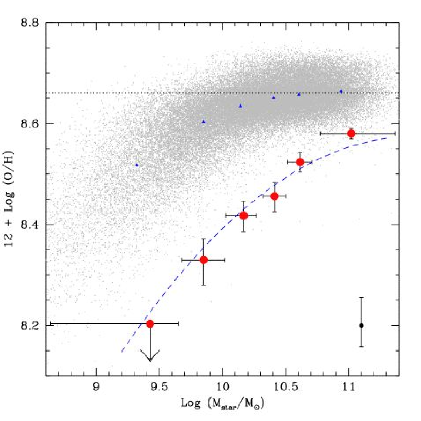
Figure 3.— The observed relation between stellar mass and oxygen abundance at $z\sim 2$ is shown by the large red circles. Each point represents the average value of 14 or 15 galaxies, with the metallicity estimated from the [N II]/$\rm H\alpha$ ratio of their composite spectrum. Horizontal bars indicate the range of stellar masses in each bin, while the vertical error bars show the uncertainty in the [N II]/$\rm H\alpha$ ratio. The additional error bar in the lower right corner shows the additional uncertainty in the $N2$ calibration itself. The dashed blue line is the best-fit mass-metallicity relation of Tremonti et al. (2004), shifted downward by 0.56 dex. The metallicities of different samples are best compared using the same calibration; we therefore show, with small grey points, the metallicities of the $\sim 53,000$ SDSS galaxies of Tremonti et al. (2004) determined with the $N2$ index. Note that the [N II]/$\rm H\alpha$ ratio saturates near solar metallicity (the horizontal dotted line). The blue triangles indicate the mean metallicity of the SDSS galaxies in the same mass bins we use for our sample; using the more reliable, low metallicity bins, our galaxies are $\sim 0.3$ dex lower in metallicity at a given mass.

4.1. Composite Ultraviolet Spectra

Given the uncertainties in the absolute metallicity scale associated with the $N2$ index, it would be highly desirable to obtain independent abundance measures for the galaxies considered here. As discussed by Rix et al. (2004), the ultraviolet spectrum of star-forming galaxies is rich in stellar spectral features which provide abundance diagnostics for the young stellar populations. The difficulty is that these are low-contrast features, usually requiring data of higher quality than can be obtained with current instrumentation. Nevertheless, it is worthwhile to examine whether the rest-frame ultraviolet spectra of the galaxies under study are consistent with the abundance trend revealed by Figure 3.

To this end we have constructed two composite spectra, each consisting of approximately 30 galaxies, by averaging the LRIS-B spectra of the galaxies in, respectively, the two lower and the two higher mass bins in Figure 3. The corresponding mean stellar masses are $\langle M_{\star}\rangle=5\times 10^{9}$ $\rm M_{\odot}$ and $\langle M_{\star}\rangle=7\times 10^{10}$ $\rm M_{\odot}$. The coarser mass binning was required to improve the S/N of the rest-UV composites to the level where the stellar absorption features which are sensitive to metallicity could be clearly discerned. The two composite spectra are shown in Figure 4, after normalization to the underlying stellar continua following the prescription by Rix et al. (2004).

Within the spectral region of 1150–1925 Å covered by the composites, the interval near 1400 Å is particularly suitable for an abundance analysis; we show this portion on an expanded scale in Figure 5. The region includes two blends of stellar photospheric lines, centered at 1370 Å and 1425 Å, whose strengths were shown by Leitherer et al. (2001) to be mostly sensitive to metallicity. The “1370” feature is a blend of O V $\lambda 1371$ and Fe V $\lambda\lambda 1360-1380$, while Si III $\lambda 1417$, C III $\lambda 1427$, and Fe V $\lambda 1430$ make up the “1425” feature. This portion of the spectra also encompasses the Si IV $\lambda\lambda 1393,1402$ doublet, which has a broad stellar P-Cygni component formed in the expanding atmospheres of late O and early B supergiants; superposed on this broad component are narrower interstellar absorption lines due to the ambient interstellar medium which lies in front of the stars.

In Figure 5 we have also reproduced synthetic spectra generated with the Starburst99 code (Leitherer et al. 1999, 2001) for the standard case of continuous star formation and Salpeter initial mass function, using in turn the two empirical stellar libraries available in the code, built from spectra of OB stars in, respectively, the Milky Way (the solar metallicity, or $Z=Z_{\odot}$, library) and the Magellanic Clouds (the MC metallicity, or $Z=1/3\,Z_{\odot}$, library). Figure 5 shows that the former is a plausible match to the composite spectrum of the higher stellar mass galaxies, while the latter is consistent with the composite UV spectrum of the galaxies in the lower stellar mass bins. We now discuss this comparison in more detail.

Focusing on the composite spectrum of the most massive galaxies (the lower panel in Figure 5), we find that the overall equivalent widths of the “1370” and “1425” photospheric features are in agreement between empirical and synthetic spectra. The comparison of the Si IV $\lambda\lambda 1393,1402$ P-Cygni component is complicated by the blending with the interstellar lines which, as is usually the case, are stronger (and blue-shifted) in starburst galaxies than in the individual stars which make up the stellar libraries. Nevertheless, the broad component of the Si IV feature has comparable optical depth to the solar metallicity Starburst99 model. Turning to the lower mass galaxies (upper panel in Figure 5), we see that all three spectral features are undetected in the lower stellar mass UV composite. The Magellanic Cloud metallicity model spectrum also shows these lines to be much reduced in strength.

The S/N ratio of the data and the subtlety of the spectral features in question limit the above comparison to qualitative statements, and we do not consider a more quantitative approach (such as a $\chi^{2}$ analysis, for example) to be warranted in the present circumstances. Nevertheless, with only the UV spectra at our disposal, we would have concluded that the galaxies with a mean stellar mass $\langle M_{\star}\rangle=7\times 10^{10}$ $\rm M_{\odot}$ have metallicity $Z\sim Z_{\odot}$ (or $12+\log{\rm(O/H)}\sim 8.6$), and that those with $\langle M_{\star}\rangle=5\times 10^{9}$ $\rm M_{\odot}$ have $Z\lesssim 1/3\,Z_{\odot}$ (or $12+\log{\rm(O/H)}\lesssim 8.1$). Given the uncertainties, these conclusions are broadly consistent with those deduced from our analysis of the [N II]/H$\alpha$ ratios.

There are other differences between the two composite UV spectra reproduced in Figure 4; for example, the interstellar absorption lines are significantly stronger in the galaxies with higher stellar mass. The strongest UV interstellar lines, Si II $\lambda 1260$, O I $\lambda 1302$+Si II $\lambda 1304$, C II $\lambda 1334$, Si II $\lambda 1526$, Fe II $\lambda 1608$, and Al II $\lambda 1670$, have rest-frame equivalent widths $W_{0}=2-3$ Å in the $\langle M^{\ast}\rangle=7\times 10^{10}$ $\rm M_{\odot}$ composite, and $W_{0}=1.5-2$ Å in the $\langle M^{\ast}\rangle=5\times 10^{9}$ $\rm M_{\odot}$ composite. Since these lines are all strongly saturated (e.g. Pettini et al. 2002), the higher equivalent widths are much more likely to be due to a larger velocity dispersion of the absorbing gas, than to an increase in the column densities of the metals. This may be related to differences in the star-formation histories of the two samples of galaxies; on average, star formation has been in progress for longer in galaxies with higher values of $\langle M_{\star}\rangle$ and presumably more kinetic energy has been deposited in their interstellar media, stirring the gas to higher velocity dispersions.

Finally, the most obvious difference between the two composite UV spectra is in the strengths of the two nebular emission lines which fall within our wavelength range, Ly$\alpha$ and C iii] $\lambda 1908$, which are much stronger in the lower stellar mass galaxies. Qualitatively, this difference is in agreement with the metallicity and kinematics differences discussed above. The C iii] $\lambda\lambda 1907,1909$ doublet is similar to [O iii] $\lambda\lambda 5007,4959$ in showing a steep inverse dependence on metallicity in the high metallicity regime—as the metallicity increases, the temperature of the H ii regions decreases and so do the relative populations of the collisionally excited levels from which these emission lines originate (e.g. Pettini & Pagel 2004). Thus, it is not surprising to find that C iii] $\lambda 1908$ is strong in the UV composite with metallicity $Z\lesssim 1/3Z_{\odot}$, and below our detection limit in the galaxies with metallicities close to solar. The dominant factor which determines the escape of resonantly scattered Ly$\alpha$ photons from a star-forming galaxy is the velocity dispersion of the interstellar gas through which the photons propagate—the larger the velocity dispersion, the smaller (and more blue-shifted) is the fraction of Ly$\alpha$ photons that escape before being absorbed by dust and turned into infrared photons (e.g. Mas-Hesse et al. 2003). Thus, the stronger Ly$\alpha$ flux of the galaxies making up the lower stellar mass composite in the top panel of Figure 4 goes hand in hand with the smaller velocity dispersion of their interstellar media, as discussed above.

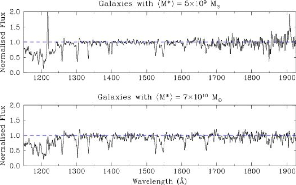
Figure 4.— Composite rest-frame UV spectra of galaxies in the two lower (top panel) and two higher (bottom panel) mass bins in our sample. The upper spectrum is the average of 30 LRIS-B spectra of galaxies with mean stellar mass $\langle M_{\star}\rangle=5\times 10^{9}$ $\rm M_{\odot}$, while 28 spectra contribute to the lower composite for which $\langle M_{\star}\rangle=7\times 10^{10}$ $\rm M_{\odot}$. The spectra have been divided by the underlying stellar continuum estimated according to the prescription by Rix et al. (2004). Differences in the stellar, interstellar, and nebular lines between the two composites are discussed in the text.

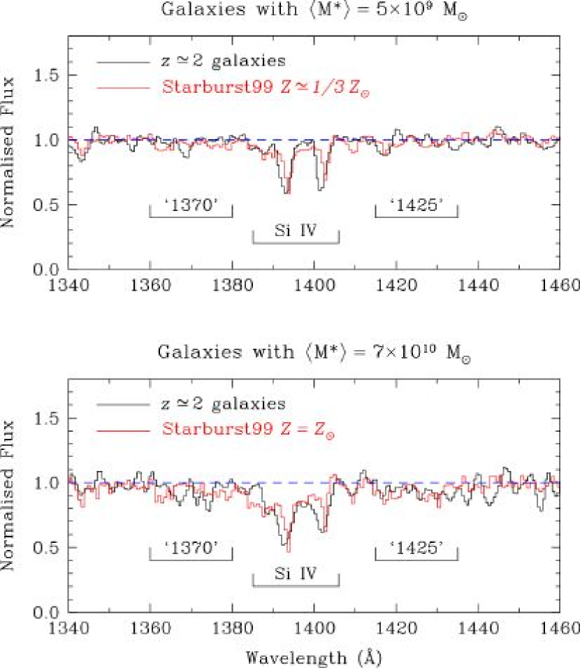
Figure 5.— Close-up of the 1400 Å region in the two composite spectra shown in Figure 4 (black histogram). This region contains two blends of stellar photospheric lines, labeled “1370” and “1425”, whose strength is thought to depend primarily on metallicity, and the Si IV $\lambda\lambda 1393,1402$ doublet which consists of a broad P-Cygni stellar absorption on which narrower interstellar lines are superposed. The red histogram shows the Starburst99 spectrum for the standard case of continuous star formation with a Salpeter IMF and ‘Magellanic Cloud’ (upper panel) or solar (lower panel) metallicities.

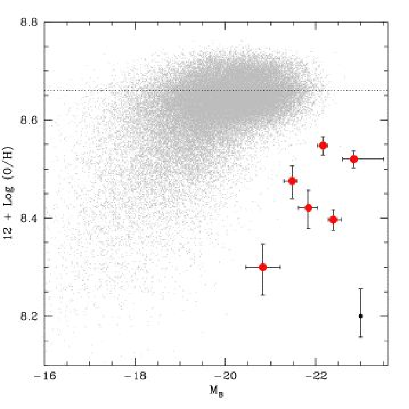
Figure 6.— The luminosity-metallicity relation at $z\gtrsim 2$. We have divided the sample into six bins by rest-frame absolute $B$ magnitude, and estimated the metallicity in each bin. The symbols are the same as in Figure 3. The points are not significantly correlated, though the faintest galaxies do have the lowest metallicities. The lack of correlation can be understood through the large variation in the optical mass-to-light ratio at high redshift. The $z\sim 2$ galaxies are $\sim 3$ magnitudes brighter than the SDSS galaxies at a given metallicity, as estimated by the [N II]/$\rm H\alpha$ ratio.

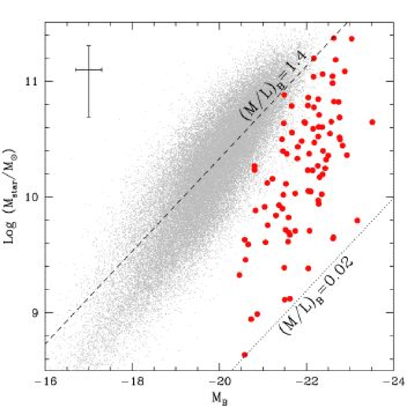
Figure 7.— Absolute rest-frame $B$ magnitude vs. stellar mass, for the individual galaxies in the $z\sim 2$ sample (large red circles) and the SDSS (small grey points). The dashed and dotted lines show constant mass-to-light ratios $M/L$; in the $z\sim 2$ sample, the total range in luminosity is narrow and $M/L$ varies by a factor of $\sim 70$ at most luminosities, while for most SDSS galaxies, $M/L$ varies by a factor of 2–5 at a given luminosity.

4.2. The Luminosity-Metallicity Relation

Because the luminosity of a galaxy is far more easily determined than its mass, there are a great many more luminosity-metallicity (L-Z) relations than mass-metallicity relations in the literature (e.g. Skillman et al. 1989; Zaritsky et al. 1994; Garnett et al. 1997; Lamareille et al. 2004; Salzer et al. 2005, to name only a few). These correlations span 11 orders of magnitude in luminosity and 2 dex in metallicity, and are seen in galaxies of all types. Both the slope and the zeropoint of the relation shift depending on the bandpass in which the correlation is determined (Salzer et al. 2005); it is traditional to use the absolute $B$ magnitude, but both the slope and the dispersion of the relation decrease as wavelength increases to the IR, probably due to decreased extinction and the closer correspondence of the infrared luminosity to stellar mass. The metallicity-luminosity relation has been observed in galaxies at redshifts up to $z\sim 1$ (Kobulnicky et al. 2003; Lilly et al. 2003; Kobulnicky & Kewley 2004; Maier et al. 2004; Liang et al. 2004), at which point the shifting of most of the strong nebular lines into the IR makes spectroscopy much more difficult. Most of these studies show that the zeropoint of the L-Z relation evolves with redshift, so that galaxies of a given luminosity have decreasing metallicity with increasing redshift. The so-far small number of metallicity-luminosity comparisons at $z>2$ confirm this trend, as high redshift galaxies are 2–4 mags brighter than local galaxies of comparable metallicity (Kobulnicky & Koo 2000; Pettini et al. 2001; Shapley et al. 2004).

We construct a luminosity-metallicity relation analogous to our mass-metallicity relation by dividing our sample of 87 galaxies into six bins by rest-frame absolute $B$ magnitude $M_{B}$, which we determine by multiplying the best-fit SED of each object by the redshifted $B$-band transmission curve. We construct a composite spectrum of the galaxies in each bin, and measure the [N II]/$\rm H\alpha$ ratio and determine the oxygen abundance in the manner described in §3.2. The results are shown in Figure 6, again including SDSS metallicities determined from the $N2$ indicator. It is immediately apparent that the correlation between luminosity and metallicity is weaker than that between mass and metallicity; the trend with luminosity is not monotonic, and is not statistically significant. A Spearman correlation test finds a 33% probability that the points are uncorrelated, giving a significance of 1$\sigma$. The faintest galaxies do have the lowest metallicities, however; any appearance of correlation is driven by this bin.

The comparison with the SDSS sample is again made difficult by the saturation of the [N II]/$\rm H\alpha$ ratio around solar metallicity, but it is clear that the high redshift galaxies have both lower metallicities (subject to the caveats discussed in §4) and higher luminosities than most of the local sample. Considering the offset of the more reliable lower metallicity bins, we see from Figure 6 that the $z\sim 2$ galaxies are approximately three magnitudes brighter than local galaxies with the same oxygen abundance. It is difficult to invert the comparison to determine the difference in metallicity between galaxies of a given luminosity in the two samples, however, since virtually all of the local galaxies as bright as the $z\sim 2$ sample have solar or greater abundances which cannot be accurately determined by the $N2$ method. In order for the best-fit L-Z relation determined by T04 to pass through the average luminosity and metallicity of our sample, it must be shifted downward by $\sim 0.9$ dex. After allowing for the $\sim 0.25$ dex systematic difference between the metallicity diagnostics used by T04 and here (as discussed in §4), we are still left with a shift of 0.6–0.7 dex between the local and high redshift samples. Our mean values are offset from other local L-Z relations by amounts ranging from $\sim 0.4$ (Skillman et al. 1989) to $\sim 1.0$ (Lamareille et al. 2004) dex. The large offsets between the various local relations are due to differences in calibration methods and sample selection; the relations are not directly comparable, and it is not yet clear which of them, if any, provides the most appropriate comparison for our sample. While it is probably a robust conclusion that the $z\sim 2$ galaxies are more metal-poor than their luminous local counterparts, a better understanding of systematic effects is required to reliably quantify the differences.

Our results are consistent with previous L-Z determinations at $z>2$, and, moreover, they are not surprising given our knowledge of the high redshift sample. Star-forming galaxies at $z\sim 2$ have lower average mass-to-light ratios $M/L$ than local galaxies, and the variation in $M/L$ at a given rest-frame optical luminosity can be as much as a factor of $\sim 70$ (Shapley et al. 2005b). This large variation in $M/L$ explains the lack of correlation in the $z\sim 2$ L-Z relation compared to the local relation. Figure 7 shows absolute magnitude $M_{B}$ plotted against stellar mass for the individual galaxies in the $z\sim 2$ and SDSS samples. The $z\sim 2$ sample is shown by large red points; at a given luminosity, $M/L$ varies by up to a factor of 70, and the range in luminosity is small, so that galaxies with a wide range of stellar masses fall in each of the six bins in luminosity. In contrast, $M_{\star}$ and $M_{B}$ are much more tightly correlated in the SDSS sample (small grey points); at a given luminosity, most of the points are within a factor of a few in $M/L$. If the fundamental correlation is between metallicity and mass, these differences in $M/L$ would shift the relation to higher luminosities and dramatically increase the scatter, as we have observed. A mass-metallicity correlation is clearly more physically meaningful than a luminosity-metallicity correlation at high redshifts; a corollary is that the local metallicity-luminosity relation is simply a result of the strong correlation between mass and luminosity at low redshift. While it is likely that an L-Z relation determined in the rest-frame IR would show a stronger correlation, investigation of this possibility must wait until a larger sample of high $z$ galaxies with both mid-IR photometry and nebular line spectra has been assembled.

5. The Origin of the Mass-Metallicity Relation

A correlation between gas-phase metallicity and stellar mass can plausibly be explained either by the tendency of lower mass galaxies to have larger gas fractions (McGaugh & de Blok 1997; Bell & de Jong 2000) and thus be less enriched, or by the preferential loss of metals from galaxies with shallow potential wells by galactic-scale winds. With the relevant information on the star, gas, and metal content of the galaxies, the two effects can be differentiated. In the simple, closed-box model of chemical evolution with no inflows or outflows, the mass fraction of metals $Z$ is a simple function of the gas fraction $\mu\equiv M_{\rm gas}/(M_{\rm gas}+M_{\star})$ and the true yield $y$, which represents the ratio of the mass of metals produced and ejected by star formation to the mass of metals locked in long-lived stars and remnants. The true yield is a function of stellar nucleosynthesis, and as in previous, similar studies (T04, Garnett 2002) we assume that it is constant (see Garnett 2002 for a discussion). The metallicity is then given by

$$Z=y\;{\rm ln}(1/\mu).$$ (2)

This equation can be inverted to determine the effective yield $y_{\rm eff}$ from the observed metallicity and gas fraction, $y_{\rm eff}=Z/{\rm ln}(1/\mu)$. If the simple model applies, $y_{\rm eff}$ will be constant for all masses and equal to the true yield $y$, while a decrease in $y_{\rm eff}$ (either with respect to the expected true yield or, more commonly, as a function of mass) is a signature of outflows or of dilution by the infall of metal-poor gas (Edmunds 1990).

T04 determined the effective yields of the SDSS galaxies by using the empirical Schmidt law (Kennicutt 1998), which relates the star formation rate per unit area to the gas surface density, to estimate gas masses. They found lower effective yields in galaxies with lower baryonic masses (the baryonic mass is expected to correlate with the dark matter content, and thus indicate the depth of the potential well; McGaugh et al. 2000), and interpreted this result as evidence for the preferential loss of metals in low-mass galaxies. We carry out a similar analysis on our sample of $z\sim 2$ galaxies. As described by Erb et al. (2006a), we use a galaxy’s $\rm H\alpha$ luminosity and the spatial extent of its $\rm H\alpha$ emission $r_{\rm H\alpha}$ (after deconvolution with the seeing point spread function) to calculate the $\rm H\alpha$ luminosity per unit area $\Sigma_{\rm H\alpha}$. We then estimate each galaxy’s gas surface density $\Sigma_{\rm gas}$ by combining the Kennicutt (1998) relation between star formation rate per unit area and gas density with the conversion from $\rm H\alpha$ luminosity to SFR from the same paper as follows:

$$\Sigma_{\rm gas}=1.6\times 10^{-27}\left(\frac{\Sigma_{\rm H\alpha}}{{\rm erg\;s^{-1}\;kpc}^{-2}}\right)^{0.71}\;{\rm M_{\odot}\;pc^{-2}}.$$ (3)

The estimated gas mass is then $M_{\rm gas}\sim\Sigma_{\rm gas}r_{\rm H\alpha}^{2}$. We next combine $M_{\rm gas}$ and $M_{\star}$ to obtain an estimate of the gas fraction $\mu$, and compute the mean value of $\mu$ in each mass bin. Although the considerable (factor of $\sim 2$) uncertainties in both the corrected $\rm H\alpha$ flux and the galaxy’s size translate into a significant uncertainty in $\mu$ for individual objects, the number of galaxies in each bin allows us to determine the mean value of $\mu$ to within $\sim 10$%.

Galaxies at low and intermediate redshifts show significant correlations between metallicity and extinction (e.g. Cortese et al. 2005; Maier et al. 2005). Galaxies at $z\sim 2$ also show a strong correlation between dust obscuration and stellar mass (and hence metallicity), as shown by Reddy et al. (2006), who use the 24 µm luminosity as observed by the Spitzer Space Telescope to infer the infrared luminosity $L_{\rm IR}$ and the extinction as parameterized by $L_{\rm IR}/L_{\rm UV}$. One implication of the work of Reddy et al. (2006) is that $E(B-V)$ as determined from the UV slope may overestimate the extinction correction for galaxies with ages less than 100 Myr. This effect can be seen in the high mean value of $E(B-V)$ for the lowest mass bin in Table 1; for galaxies with ages greater than 100 Myr in the current sample, $E(B-V)$ and stellar mass are correlated with 4$\sigma$ significance. This overestimation of the extinction in young galaxies has a negligible effect on our current analysis; we estimate that it will lead to an overestimation of the SFRs by a typical factor of $\sim 1.2$, considerably less than other uncertainties. Only the lowest mass bin is affected, since it is the only one that contains a significant number of young objects; because we derive only an upper limit on the mean metallicity of the galaxies in this bin, it does not affect our conclusions.

As in the local universe (McGaugh & de Blok 1997; Bell & de Jong 2000), there is a strong trend of decreasing gas fraction with increasing stellar mass. The lowest mass bin in the sample has a mean gas fraction $\langle\mu\rangle=0.85$, while the highest mass bin has $\langle\mu\rangle=0.22$. The median value of $\mu$ in our sample is $\sim 0.5$, significantly higher than the corresponding median value of $\sim 0.2$ for the SDSS galaxies considered by T04. The low metallicities, low stellar masses and high gas fractions of the objects in the lowest mass bin suggest that they are young objects just beginning to form stars; this is also indicated by the ages from the SED modeling (see Table 1). The correlations between age and other properties are discussed in detail by Erb et al. (2006a) in the context of the comparison of stellar and dynamical masses.

A consequence of the large gas fractions of the low stellar mass bins is that the baryonic mass $M_{\rm gas}+M_{\star}$ of the galaxies in the sample spans a much smaller range than the stellar mass. The difference in mean stellar mass between the highest and lowest mass bins is a factor of 39, while the difference in mean baryonic mass between the same bins is only a factor of six. This relatively small range in baryonic mass also limits our ability to detect differential loss of metals as a function of mass. We show the variations of $M_{\star}$, $M_{\rm gas}$, and $M_{\rm bar}$ with metallicity in Figure 8. Notably, the increase in baryonic mass along our sequence of six bins is driven almost entirely by the increase in stellar mass, while the gas mass remains relatively constant. This is because the average star formation rate and $\rm H\alpha$ luminosity vary much less than the average stellar mass across the bins; in particular, galaxies in the lowest mass bin have higher than average SFRs. This may seem contrary to the trend of increasing SFR at brighter $K$ magnitudes found by Reddy et al. (2005), but we account for the difference both because we are less likely to detect $\rm H\alpha$ emission in $K$-faint galaxies unless it is especially strong (as discussed by Erb et al. 2006a, b) and because galaxies are more likely to be detected in the $K$-band if they have high SFRs. Reddy et al. (2006) also show that the correlation of stellar mass and bolometric luminosity is relatively weak, and that low stellar mass galaxies span a wide range in $L_{\rm bol}$. For present purposes, there is a lower limit on the gas masses we are able to detect corresponding to our $\rm H\alpha$ flux limit, and the absence of galaxies with both low stellar masses and low gas masses is probably a selection effect. We also note that the dynamical masses derived from the $\rm H\alpha$ line widths are a better match to the baryonic masses than the stellar masses, with $M_{\rm dyn}\gg M_{\star}$ for the objects in the lowest mass bin. Erb et al. (2006a) discuss this comparison in detail.

The mean gas fractions and effective yields for each mass bin are given in Table 2. In contrast to the SDSS sample, there is no decline in the effective yield with decreasing baryonic mass; in fact we see the opposite, as $y_{\rm eff}$ increases slightly with decreasing mass. The points in each panel of Figure 9 show the metallicity $Z$ in each mass bin plotted against the mean gas fraction $\mu$, with decreasing gas fraction from left to right to show the increase in $Z$ as $\mu$ declines. We first discuss the data in the context of the closed box model with no inflows or outflows. For such a model, lines of constant yield are curves given by Eq. 2. The uppermost (black) curve on each of the three plots shows the variation of $Z$ with gas fraction in this model for three different values of the true yield $y$; from left to right we show $y$ equal to our observed effective yield $y_{\rm eff}=0.008\sim 0.6\,Z_{\odot}$, solar yield $y=0.0126$, and a supersolar yield $y=1.5\,Z_{\odot}$. The points are formally consistent with the $y\sim 0.6\,Z_{\odot}$ model in the left panel, as the measured value of $y_{\rm eff}$ in each bin is within 1$\sigma$ of the weighted mean $y_{\rm eff}=0.008$ in 4 of the bins, and within 2$\sigma$ of this value in the fifth (we do not consider the lowest mass bin, for which we find only an upper limit on $Z$ and $y_{\rm eff}$); however, the systematic tendency of the lower mass points to fall above the black line indicates that the model is not a good fit. A $\chi^{2}$ test confirms this, giving a value of 9.

Given the ubiquitous signature of galactic-scale outflows in the kinematics of the $z\sim 2$ galaxies, we now consider the effects of such outflows on the metallicities of the galaxies. To address this question we modify the simple model to include gas outflow at rate $\dot{M}$ $\rm M_{\odot}\;{\rm yr}^{-1}$, which is a fraction $f$ of the star formation rate; note that in this model the outflow rate does not directly depend on the mass of the galaxy. We assume that the metallicity of the outflowing gas is the same as the metallicity of the gas that remains in the H II regions in the galaxy. It can then be shown that the metallicity is given by

$$Z=y\;(1+f)^{-1}\;{\rm ln}\;[1+(1+f)(\mu^{-1}-1)].$$ (4)

Observations at low and high redshift suggest that $\dot{M}$ is comparable to the star formation rate, and may be higher (e.g. Martin 1999; Pettini et al. 2000; Martin 2003). The curves in each panel of Figure 9 show the evolution of $Z$ with gas fraction for, from top to bottom, $f=0$ (black; the closed box model), 0.5 (purple), 1 (blue), 2 (green), and 4 (red). A decrease in $y_{\rm eff}$ with decreasing gas fraction such as we have inferred is a general feature of models with constant $\dot{M}/$SFR; more specifically, from comparison with the points in each panel, it is apparent that the data are best matched by a model with supersolar yield $y\sim 1.5\,Z_{\odot}$ and a high outflow rate $\dot{M}\sim 4\times$SFR (the red line in the righthand panel). We caution that the uncertainties in both metallicity and gas fraction are too large to distinguish between the above models with confidence; nevertheless the best-fitting model is not implausible, as we discuss below.

An outflow rate of several times the star formation rate has already been suggested by observations of the the lensed LBG MS1512-cB58; Pettini et al. (2002) found a value of $\dot{M}$ higher than the star formation rate using conservative assumptions for the size of the galaxy and outflow velocity. This scenario is also in good agreement with observations and predictions of the enrichment of the intracluster medium (ICM). The ICM contains several times more mass in baryons than is found in the cluster galaxies themselves, and thus it contains most of the metals in clusters as well (e.g. Mushotzky & Loewenstein 1997). Recent models for the enrichment of the ICM (De Lucia et al. 2004; Nagashima et al. 2005) use feedback from supernovae to transport metals out of galaxies, finding that enrichment of the ICM occurs at high redshift, with of order half of the metals produced by $z\sim 2$, and that half or more of the metals in the ICM are produced in massive galaxies ($L\gtrsim L_{\ast}$, Nagashima et al. 2005; or baryonic mass $\gtrsim 10^{10}\,h^{-1}$ $\rm M_{\odot}$, De Lucia et al. 2004). These models also require either a top-heavy IMF in starbursts or a significantly enhanced yield in order to reproduce the observed metal abundances in clusters; some such variant IMF is a feature of many models of star formation and chemical enrichment in clusters (e.g. Zepf & Silk 1996; Finoguenov et al. 2003; Tornatore et al. 2004). The supersolar yield suggested by the best-fitting model shown in Figure 9 may support such a scenario, although we emphasize that our data do not require an IMF with more high-mass stars than the Chabrier (2003) IMF we use here. Such an IMF, when combined with estimates of yields from stellar nucleosynthesis (e.g. Meynet & Maeder 2002), results in a metal yield that is solar or higher.

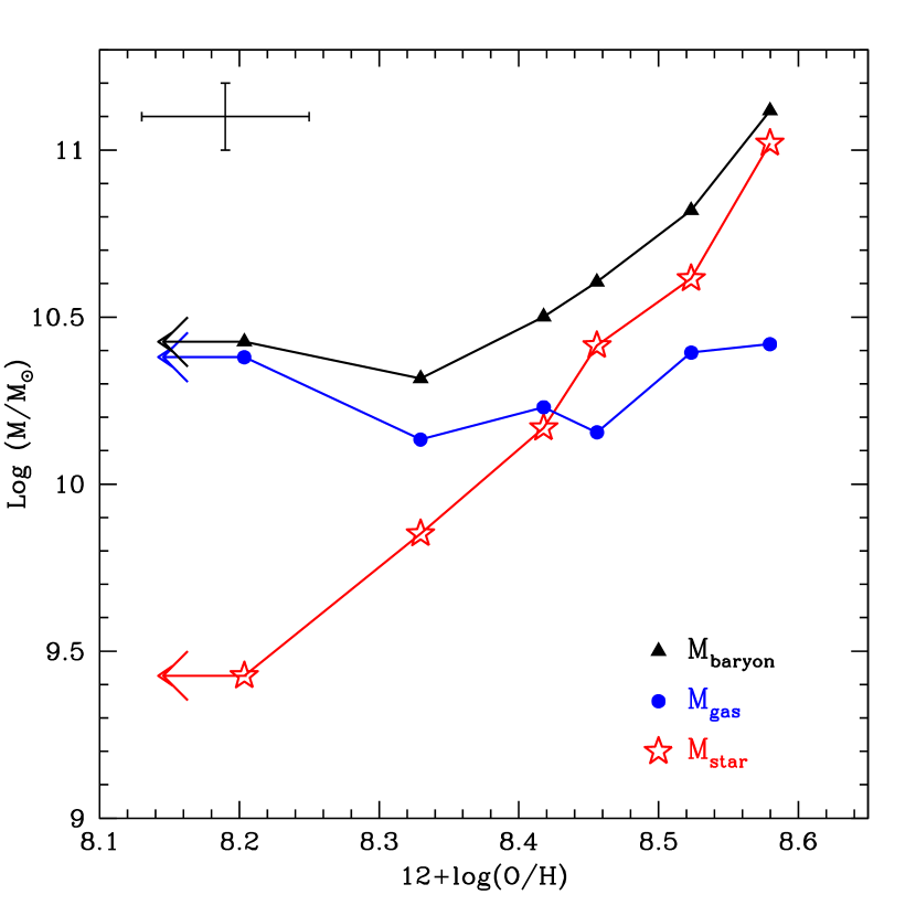
Figure 8.— The variation of stellar, gas, and baryonic mass in each of the six bins with metallicity. Across the observed range in oxygen abundance, stellar mass increases strongly, baryonic mass increases weakly, and gas mass remains approximately constant. We thus see an increase in metallicity with decreasing gas fraction. The strong correlation between stellar mass and age means that metallicity also increases with the age of the stellar population. The error bars at upper left show typical uncertainties in gas and baryonic masses and metallicities; uncertainties in stellar masses are smaller.

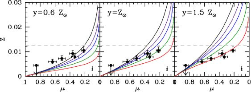
Figure 9.— The points in each panel show the mean metallicity $Z$ in each mass bin, plotted against the mean gas fraction $\mu$. Gas fraction decreases from left to right, to show the increase in metallicity with decreasing gas fraction. The curves illustrate the variation of $Z$ with $\mu$ for three different values of the true yield: from left to right, $y=0.6\,Z_{\odot}$ (our observed effective yield), $y=Z_{\odot}$, and $y=1.5\,Z_{\odot}$. Within each panel, the curves show varying values of the mass outflow rate $\dot{M}$, parameterized as a fraction $f$ of the star formation rate. From top to bottom in each panel, the curves correspond to $f=0$ (black; the closed box model), 0.5 (purple), 1 (blue), 2 (green) and 4 (red). The data are best matched by a model with supersolar yield and an outflow rate $\dot{M}\sim 4\times$SFR. The horizontal dashed grey line corresponds to solar metallicity, and the small error bar in the lower right corner of each panel shows the systematic uncertainty in the metallicity calibration.

5.1. Redshift Evolution of the Mass-Metallicity Relation

With estimates of the gas fractions in hand we now return to the $\sim 0.3$ dex offset between the local and $z\sim 2$ mass-metallicity relations. There are several possible reasons for this factor of $\sim 2$ difference. The magnitude of the offset itself is not well-determined because of the uncertainty in our metallicity scale indicated by the offsets between the [O III]/$\rm H\beta$ and [N II]/$\rm H\alpha$ ratios relative to the SDSS galaxies seen in Figure 1. The effects of these offsets cannot be quantified reliably without detailed modeling of a larger sample of galaxies with all four emission lines, but meanwhile we can use several techniques to estimate the possible uncertainty in metallicity that may result. We have another method of determining the metallicity of the four galaxies with all four emission lines in the $O3N2$ index of Pettini & Pagel (2004): $O3N2\equiv\log$ {[O III]$\lambda 5007/\rm H\beta)/($[N II$]\lambda 6583/\rm H\alpha)$}. Pettini & Pagel (2004) find that $O3N2$ varies with oxygen abundance as

$${\rm 12+log\;(O/H)}=8.73-0.32\times O3N2.$$ (5)

Using this calibration to determine the metallicities of the four galaxies with all four lines, we find oxygen abundances that are 0.17 dex lower on average than those determined using [N II]/$\rm H\alpha$. This is one plausible estimate of the metallicity uncertainty due to the differing physical conditions in the H II regions of the $z\sim 2$ galaxies. We can obtain another by assuming that the observed shift in the [O III]/$\rm H\beta$ and [N II]/$\rm H\alpha$ diagram is entirely in the [N II]/$\rm H\alpha$ direction; then the relatively shallow slope of the relationship between [N II]/$\rm H\alpha$ and (O/H) leads to a maximum offset in metallicity of $\sim 0.3$ dex. The effect of an offset in the [O III]/$\rm H\beta$ and [N II]/$\rm H\alpha$ diagram on metallicity determinations is considered in detail by Shapley et al. (2005a), and we refer the reader to Section 5.3 of that paper for a discussion. These authors consider the effect of a harder ionizing spectrum in high redshift galaxies, and conclude that this could plausibly lead to a factor of $\sim 1.5$–2 uncertainty in metallicity.

Another possible issue is that the SDSS metallicities are biased toward the innermost regions of the galaxies observed, where the spectrograph fibers were positioned. According to a recent re-analysis of this effect by Ellison & Kewley (2005), this fact alone can account for a $\sim 0.15$ dex offset between nuclear and global (i.e., integrated over the whole galaxy) metallicities. However, this effect may be mitigated by the fact that our global spectra are also biased toward the galaxies’ central regions, which have the highest surface brightness. We conclude that the uncertainty in the metallicity offset between the $z\sim 2$ and local galaxies is approximately a factor of two, about the same as the offset itself.

There are reasons to believe that there may be a real evolutionary offset in the mass-metallicity relation, and we proceed with the discussion under this assumption. As described above, we find that the galaxies in our sample have an average gas fraction more than two times higher than the galaxies studied by T04, placing them at an earlier stage in the process of converting their gas to stars. Given this less evolved state, it is not surprising that they should have lower gas-phase metallicities. Redshift evolution of the mass-metallicity relation has also recently been investigated by Savaglio et al. (2005) with a sample of galaxies at $0.4<z<1$, finding that a galaxy of a given stellar mass tends to have lower metallicity at $z\sim 0.7$ than at $z\sim 0$. Using the SDSS relation of T04, their sample at $z\sim 0.7$, and the $z\sim 2$ galaxies presented by Shapley et al. (2004), they develop an empirical model for the redshift evolution of the relation. This model predicts metallicities an average of $\sim 0.2$ dex higher than we observe, though at least some of this offset is likely to be due to the different metallicity indicators used (it is not possible to place our sample and that of Savaglio et al. (2005) on the same metallicity scale, as an accurate conversion between the two indicators used has not yet been established for the samples in question). Such a shift to lower metallicities (or higher masses) with increasing redshift can qualitatively be explained via a scenario in which star formation takes place over a more protracted period in lower mass galaxies. This scenario is consistent with our results; we find that the more massive galaxies in our sample have smaller gas fractions, and are thus likely to exhaust their gas supply before the less massive galaxies.

The Savaglio et al. (2005) model also predicts a steeper relation at $z\sim 2$ than we have observed; this is a consequence of their assumption that the shape of the T04 relation remains unchanged but shifts to higher masses, whereas we find that our data is well-approximated by the T04 relation shifted to lower metallicities at the same stellar mass. In physical terms, the slope of the stellar mass-metallicity relation depends on both the yield and the presence or absence of outflows (and inflows). As shown in Figure 9, a closed box model such as that assumed by Savaglio et al. (2005) results in a steep relation between metallicity and gas fraction (and stellar mass), while the $z\sim 2$ data are better described by the shallower slope of a model with significant outflows.

While comparisons between the metallicities of star-forming galaxies at high and low redshift are of obvious interest, it is very likely that our sample and that of T04 do not form an evolutionary sequence. The likely descendants of the $z\sim 2$ sample can be identified by comparing their clustering properties, evolved to $z\sim 0$, with those of objects in the local universe; such a comparison shows that early-type galaxies in the SDSS match the clustering properties of the $z\sim 2$ sample, while the later-type star-forming objects studied by T04 are too weakly clustered to be the descendants of the $z\sim 2$ population (Adelberger et al. 2005b). In this sense it is more relevant to compare the metallicities of the $z\sim 2$ galaxies with local early-type objects than with star-forming galaxies at $z\sim 0$, though such a comparison would undoubtedly be complicated by systematic offsets resulting from the very different methods used to determine metal abundances in elliptical galaxies (usually absorption features in the integrated spectra of old stellar populations). Broadly speaking, however, most early-type galaxies in the SDSS with $M_{\star}>10^{10}$ $\rm M_{\odot}$ have metallicities ranging from $Z\sim 0.6\,Z_{\odot}$ to $Z\sim 1.5\,Z_{\odot}$ (Gallazzi et al. 2005); these results are consistent with the probable final stellar masses and metallicities of the $z\sim 2$ galaxies.

Substantial uncertainties in the mass-metallicity relation at $z\sim 2$ remain, of course. It is important to confirm the trend in metallicity with additional measurements and with abundance indicators that use a broader set of emission lines. The absolute values of the abundances in the sample are uncertain, and the improved understanding of the galaxies’ physical conditions that will result from a larger sample of lines will be essential for determining this absolute scale. Furthermore, our derivation of the gas masses and gas fractions is indirect, and assumes that the Schmidt law takes the same form at $z\sim 2$ as in the local universe. This has not yet been tested, although the one similar galaxy with a direct measurement of the gas mass, the lensed $z=2.7$ LBG MS1512-cB58, appears to be consistent with the local Schmidt law (Baker et al. 2004). As long as some form of the Schmidt law applies, our results will be qualitatively similar. A related question concerns the appropriateness of the gas masses derived from the Schmidt law. These represent only the gas associated with current star formation, and are therefore almost certainly an underestimate of the total gas masses. In a typical disk galaxy today, $\sim 40$% of the gas mass is not included by the Schmidt law (Martin & Kennicutt 2001); this fraction could plausibly be higher in the young starbursts in our sample. It is not clear how or if this gas affects the metal enrichment and star formation. Given our lack of information on this gas, we do not consider it. T04 discussed these questions of gas masses derived from the Schmidt law in somewhat more detail, but arrived at similar conclusions.

Our simple model for the effect of winds on gas-phase abundances assumes that the metallicity of the outflowing gas is the same as the observed abundances in the galaxy; this may not be correct. Metal-enhanced hot winds have been observed in X-rays in local starbursts; in dwarf galaxies, such winds may carry away nearly all the oxygen produced by the burst (Martin et al. 2002). Such a metal-enhanced outflow would increase metal losses for a given outflow rate; thus it may be possible to produce the relative shallow relationship between $Z$ and $\mu$ that we have observed with a mass outflow rate smaller than the value $\dot{M}\sim 4\times$SFR we find above.

We also consider the possibility, discussed in §3.1 and §4, that we have underestimated the stellar masses of the galaxies with the smallest $M_{\star}$ by a factor of a few. This would primarily affect the objects in the lowest mass bins, and would result in a decrease in the gas fraction and a decrease in the effective yield. A factor of three increase in the stellar mass of the galaxies in the two lowest mass bins would result in a decrease in $y_{\rm eff}$ of approximately a factor of two for those bins; this is enough to remove the observed trend of decreasing $y_{\rm eff}$ with increasing stellar mass, and results instead in an approximately constant effective yield, roughly consistent with the closed box model. Given the significant evidence for strong outflows in these galaxies, however, we regard the best-fit model obtained above as more plausible.

Finally, the sample of $z\sim 2$ galaxies considered here is by no means complete. The UV-selection technique is most likely to miss galaxies that are very dusty or have little current star formation; Reddy et al. (2005) show that there is relatively little overlap ($\sim 12$%) between the UV-selected sample and $z\sim 2$ galaxies selected by their $J-K_{s}>2.3$ colors (Distant Red Galaxies, or DRGs; Franx et al. 2003). This technique selects galaxies with a strong optical break, due to either an evolved stellar population or strong reddening (e.g. Papovich et al. 2005). Little is known about the metallicities of the DRGs. A few rest-frame optical spectra of brighter DRGs with $K<20$ have presented by van Dokkum et al. (2004, 2005); these suggest approximately solar metallicities, although they frequently show evidence for AGN or shock ionization. It will be extremely difficult to measure metallicities for passively evolving galaxies at high redshift, since they lack strong emission lines. Massive galaxies that have consumed or expelled most of their gas might be expected to be among the most metal-rich objects at high redshift. Dusty, rapidly star-forming galaxies are likely to have large gas masses, but their metallicities will depend on how many generations of stars have enriched the gas. There is probably a range of metallicities within this population. Some confirmation of this can be found in Figure 15 of Reddy et al. (2006), who plot inferred gas fraction against stellar mass for near-IR selected galaxies as well as for UV-selected galaxies similar to those considered here. All samples considered follow the same trend of decreasing gas fraction with increasing stellar mass, with the DRGs at the high mass and low gas fraction end of the spectrum. This suggests that galaxies selected by near-IR techniques may also follow a similar mass-metallicity relation to that discussed here, with a possible extension to higher metallicities for the oldest and most massive objects. It will be interesting to see if this proves to be true when larger samples of metallicity measurements become available.

In summary, the $z\sim 2$ galaxies show a strong trend in oxygen abundance over a range of only a factor of $\sim 6$ in baryonic mass. The effective yield increases slightly with decreasing mass, rather than decreasing as would be expected if low mass galaxies lost a larger fraction of their metals to outflows. We conclude that the mass-metallicity relation at high redshift is primarily a product of varying stages of galaxy evolution, caused by the increase in metallicity as gas is converted into stars and metals are returned to the remaining gas. It may be modulated by metal loss from strong outflows in galaxies of all masses, which results in a shallower increase of metallicity with decreasing gas fraction than predicted by the closed box model. There is no evidence for preferential loss of metals from lower mass galaxies, as has been inferred in the local universe, although the small mass range spanned by our sample limits our sensitivity to such an effect.

6. Summary and Conclusions

We have used composite $\rm H\alpha$ + [N II] spectra of 87 star-forming galaxies at $z\gtrsim 2$, divided into six bins by stellar mass, to study the correlation between stellar mass and metallicity at high redshift. Our conclusions are summarized as follows.

1. There is a strong correlation between stellar mass and metallicity at $z\gtrsim 2$, as the quantity $12+\rm log(O/H)$ increases monotonically from $<8.2$ for galaxies with $\langle M_{\star}\rangle=2.7\times 10^{9}$ $\rm M_{\odot}$ to 8.6 for galaxies with $\langle M_{\star}\rangle=1.0\times 10^{11}$ $\rm M_{\odot}$. The relation is offset by $\sim 0.3$ dex from the local mass-metallicity relation, in the sense that galaxies of a given stellar mass have lower metallicities at high redshift. The absolute values of the oxygen abundances are uncertain, but the trend is unlikely to be due to systematic effects such as AGN contamination, hidden stellar mass, or variations in the ionization parameter of the H II regions.

2. Rest-frame $B$-band luminosity and metallicity are not significantly correlated. The $z\sim 2$ galaxies are systematically brighter than local star-forming galaxies spanning the same range in stellar mass, showing that they have smaller mass-to-light ratios $M/L$. At a given metallicity, local galaxies are $\sim 3$ magnitudes fainter than the $z\sim 2$ sample. The known large scatter in the rest-frame optical $M/L$ at $z\sim 2$ accounts for the lack of correlation between luminosity and metallicity, and indicates that the correlation with stellar mass is (as expected) more fundamental.

3. We use the Schmidt law to estimate the gas masses and gas fractions of the $z\sim 2$ galaxies, finding that the gas fraction increases substantially with decreasing stellar mass. The lowest mass bin in the sample has a mean gas fraction of 85%, while the highest stellar mass bin has a fraction of 20%. Our median gas fraction is $\sim 50$%, as compared to $\sim 20$% in local star-forming galaxies. Galaxies with low stellar masses, low metallicities and high gas fractions also have young ages. A consequence of the trend in gas fraction with stellar mass is a much smaller range in baryonic mass (a factor of 6) than stellar mass (a factor of 39) across the sample.

4. The observed metallicities and gas fractions allow an estimate of the effective yield in each mass bin. In contrast to the results of a similar study in the local universe, we find no decrease in $y_{\rm eff}$ at low masses; instead, $y_{\rm eff}$ increases slightly with decreasing mass. Qualitatively, such an increase is a feature of models in which galaxies of all masses lose metals from outflows. More quantitatively, comparison with simple models shows that the observed variation of metallicity with gas fraction is best described by a model with supersolar yield and an outflow rate $\sim 4$ times higher than the star formation rate. We conclude that the mass-metallicity relation at high redshift is caused by the increase in metallicity as gas is converted to stars, and may be modulated by strong outflows in galaxies of all masses. Our ability to detect differential metal loss as a function of mass is limited by the small range of baryonic masses spanned by the galaxies in the sample, but there is no evidence for preferential loss of metals from low mass galaxies as is suggested locally.

Much remains to be done in order to improve upon the substantial uncertainties inherent in the present work. Independent measurements of the gas masses of galaxies at high redshift, though very difficult, are essential to determine whether our derived gas fractions and effective yields are valid. Additional metallicity measurements, based on other indicators that use a wider set of emission lines, are needed to confirm the trend with stellar mass revealed by the $N2$ index, to provide a better understanding of the physical conditions in the H II regions, and to establish a secure absolute calibration of the metallicity scale. Further investigation of the question of differential metal loss from outflows at high redshift requires observations of fainter galaxies with smaller potential wells, to expand the dynamic range in baryonic mass. We anticipate that all of these measurements will greatly increase our understanding of the interplay between stars and gas, within and outside of galaxies, at high redshift.

Table 1Mean Stellar Masses and Stellar Population Properties

Bin	N	$\langle z\rangle$	${\cal R}$	$K_{s}$	$M_{B}$	Stellar Mass	SFR	Age	E(B-V)
						($10^{10}$ $\rm M_{\odot}$)	($\rm M_{\odot}\;{\rm yr}^{-1}$)	(Myr)
1	15	2.36	24.20 $\pm$ 0.72	21.51 $\pm$ 0.69	-21.27 $\pm$ 0.73	0.27 $\pm$ 0.15	55 $\pm$ 52	180 $\pm$ 276	0.19 $\pm$ 0.09
2	15	2.27	23.96 $\pm$ 0.81	21.03 $\pm$ 0.61	-21.66 $\pm$ 0.59	0.71 $\pm$ 0.17	24 $\pm$ 10	448 $\pm$ 374	0.14 $\pm$ 0.07
3	15	2.21	24.01 $\pm$ 0.72	20.86 $\pm$ 0.47	-21.82 $\pm$ 0.58	1.5 $\pm$ 0.3	30 $\pm$ 21	968 $\pm$ 944	0.11 $\pm$ 0.08
4	14	2.28	23.97 $\pm$ 0.62	20.54 $\pm$ 0.49	-22.15 $\pm$ 0.51	2.6 $\pm$ 0.4	28 $\pm$ 17	1026 $\pm$ 864	0.16 $\pm$ 0.07
5	14	2.21	23.93 $\pm$ 0.60	20.16 $\pm$ 0.38	-22.33 $\pm$ 0.51	4.1 $\pm$ 0.6	47 $\pm$ 30	1311 $\pm$ 790	0.17 $\pm$ 0.09
6	14	2.26	24.32 $\pm$ 0.55	20.05 $\pm$ 0.40	-22.30 $\pm$ 0.44	10.5 $\pm$ 5.4	47 $\pm$ 24	2409 $\pm$ 591	0.19 $\pm$ 0.06

Table 2Oxygen Abundances and Gas Fractions

Bin	Stellar Mass	$F_{\rm H\alpha}$	$F_{[\rm NII]}$	$N2$	12 + log(O/H)	$M_{\rm bar}$	$\mu_{\rm gas}$	$y_{\rm eff}$
	($10^{10}$ $\rm M_{\odot}$)	($10^{-17}$ erg s-1 cm-2)	($10^{-17}$ erg s-1 cm-2)			($10^{10}$ $\rm M_{\odot}$)
1	0.27 $\pm$ 0.15	$20.5\pm 0.5$	$<1.2$	$<-1.22$	$<8.20$	2.7$\pm$1.7	0.85 $\pm$ 0.12	$<0.027$
2	0.71 $\pm$ 0.17	$13.9\pm 0.3$	$1.4\pm 0.2$	$-1.00^{+0.07}_{-0.09}$	$8.33^{+0.07}_{-0.07}$	2.1$\pm$0.6	0.63 $\pm$ 0.12	0.013$\pm$0.003
3	1.5 $\pm$ 0.3	$18.7\pm 0.4$	$2.7\pm 0.3$	$-0.85^{+0.05}_{-0.06}$	$8.42^{+0.06}_{-0.05}$	3.2$\pm$1.1	0.48 $\pm$ 0.19	0.010$\pm$0.002
4	2.6 $\pm$ 0.4	$15.9\pm 0.4$	$2.6\pm 0.3$	$-0.78^{+0.05}_{-0.05}$	$8.46^{+0.06}_{-0.05}$	4.0$\pm$0.9	0.33 $\pm$ 0.12	0.007$\pm$0.001
5	4.1 $\pm$ 0.6	$24.3\pm 0.5$	$5.3\pm 0.4$	$-0.66^{+0.03}_{-0.04}$	$8.52^{+0.06}_{-0.05}$	6.6$\pm$1.1	0.36 $\pm$ 0.10	0.009$\pm$0.002
6	10.5 $\pm$ 5.4	$27.0\pm 0.4$	$7.4\pm 0.3$	$-0.56^{+0.02}_{-0.02}$	$8.58^{+0.06}_{-0.04}$	13.1$\pm$5.6	0.22 $\pm$ 0.11	0.007$\pm$0.001

References

- Adelberger et al. (2005) Adelberger, K. L., Shapley, A. E., Steidel, C. C., Pettini, M., Erb, D. K., & Reddy, N. A. 2005, ApJ, 629, 636
- Adelberger et al. (2005b) Adelberger, K. L., Steidel, C. C., Pettini, M., Shapley, A. E., Reddy, N. A., & Erb, D. K. 2005b, ApJ, 619, 697
- Adelberger et al. (2003) Adelberger, K. L., Steidel, C. C., Shapley, A. E., & Pettini, M. 2003, ApJ, 584, 45
- Asplund et al. (2004) Asplund, M., Grevesse, N., Sauval, A. J., Allende Prieto, C., & Kiselman, D. 2004, A&A, 417, 751
- Baker et al. (2004) Baker, A. J., Tacconi, L. J., Genzel, R., Lehnert, M. D., & Lutz, D. 2004, ApJ, 604, 125
- Baldwin et al. (1981) Baldwin, J. A., Phillips, M. M., & Terlevich, R. 1981, PASP, 93, 5
- Barmby et al. (2004) Barmby, P., Huang, J.-S., Fazio, G. G., Surace, J. A., Arendt, R. G., Hora, J. L., Pahre, M. A., Adelberger, K. L., Eisenhardt, P., Erb, D. K., Pettini, M., Reach, W. T., Reddy, N. A., Shapley, A. E., Steidel, C. C., Stern, D., Wang, Z., & Willner, S. P. 2004, ApJS, 154, 97
- Bell & de Jong (2000) Bell, E. F. & de Jong, R. S. 2000, MNRAS, 312, 497
- Benson et al. (2003) Benson, A. J., Bower, R. G., Frenk, C. S., Lacey, C. G., Baugh, C. M., & Cole, S. 2003, ApJ, 599, 38
- Bresolin et al. (2005) Bresolin, F., Schaerer, D., González Delgado, R. M., & Stasińska, G. 2005, A&A, 441, 981
- Bruzual & Charlot (2003) Bruzual, G. & Charlot, S. 2003, MNRAS, 344, 1000
- Calzetti et al. (2000) Calzetti, D., Armus, L., Bohlin, R. C., Kinney, A. L., Koornneef, J., & Storchi-Bergmann, T. 2000, ApJ, 533, 682
- Chabrier (2003) Chabrier, G. 2003, PASP, 115, 763
- Cortese et al. (2005) Cortese, L., Boselli, A., Buat, V., Gavazzi, G., Boissier, S., Gil de Paz, A., Seibert, M., Madore, B. F., & Martin, D. C. 2005, ApJ, in press, astro-ph/0510165
- De Lucia et al. (2004) De Lucia, G., Kauffmann, G., & White, S. D. M. 2004, MNRAS, 349, 1101
- Dekel & Woo (2003) Dekel, A. & Woo, J. 2003, MNRAS, 344, 1131
- Denicoló et al. (2002) Denicoló, G., Terlevich, R., & Terlevich, E. 2002, MNRAS, 330, 69
- Dopita (2005) Dopita, M. A. 2005, in AIP Conf. Proc. 761: The Spectral Energy Distributions of Gas-Rich Galaxies: Confronting Models with Data, 203, astro-ph/0502339
- Edmunds (1990) Edmunds, M. G. 1990, MNRAS, 246, 678
- Ellison & Kewley (2005) Ellison, S. L. & Kewley, L. J. 2005, astro-ph/0508627
- Ellison et al. (2000) Ellison, S. L., Songaila, A., Schaye, J., & Pettini, M. 2000, AJ, 120, 1175
- Erb et al. (2003) Erb, D. K., Shapley, A. E., Steidel, C. C., Pettini, M., Adelberger, K. L., Hunt, M. P., Moorwood, A. F. M., & Cuby, J. 2003, ApJ, 591, 101
- Erb et al. (2006a) Erb, D. K., Steidel, C. C., Shapley, A. E., Pettini, M., Reddy, N. A., & Adelberger, K. L. 2006a, ApJ, submitted
- Erb et al. (2006b) Erb, D. K., Steidel, C. C., Shapley, A. E., Pettini, M., Reddy, N. A., & Adelberger, K. L. 2006b, ApJ, submitted
- Finoguenov et al. (2003) Finoguenov, A., Burkert, A., & Böhringer, H. 2003, ApJ, 594, 136
- Franx et al. (2003) Franx, M., Labbé, I., Rudnick, G., van Dokkum, P. G., Daddi, E., Förster Schreiber, N. M., Moorwood, A., Rix, H., Röttgering, H., van de Wel, A., van der Werf, P., & van Starkenburg, L. 2003, ApJ, 587, L79
- Gallazzi et al. (2005) Gallazzi, A., Charlot, S., Brinchmann, J., White, S. D. M., & Tremonti, C. A. 2005, MNRAS, 362, 41
- Garnett (2002) Garnett, D. R. 2002, ApJ, 581, 1019
- Garnett et al. (2004) Garnett, D. R., Kennicutt, R. C., & Bresolin, F. 2004, ApJ, 607, L21
- Garnett et al. (1997) Garnett, D. R., Shields, G. A., Skillman, E. D., Sagan, S. P., & Dufour, R. J. 1997, ApJ, 489, 63
- Heckman et al. (1990) Heckman, T. M., Armus, L., & Miley, G. K. 1990, ApJS, 74, 833
- Hernquist & Springel (2003) Hernquist, L. & Springel, V. 2003, MNRAS, 341, 1253
- Kauffmann et al. (2003) Kauffmann, G., Heckman, T. M., Tremonti, C., Brinchmann, J., Charlot, S., White, S. D. M., Ridgway, S. E., Brinkmann, J., Fukugita, M., Hall, P. B., Ivezić, Ž., Richards, G. T., & Schneider, D. P. 2003, MNRAS, 346, 1055
- Kennicutt (1998) Kennicutt, R. C. 1998, ApJ, 498, 541
- Kennicutt et al. (2003) Kennicutt, R. C., Bresolin, F., & Garnett, D. R. 2003, ApJ, 591, 801
- Kewley & Dopita (2002) Kewley, L. J. & Dopita, M. A. 2002, ApJS, 142, 35
- Kewley et al. (2001a) Kewley, L. J., Dopita, M. A., Sutherland, R. S., Heisler, C. A., & Trevena, J. 2001a, ApJ, 556, 121
- Kewley et al. (2001b) Kewley, L. J., Heisler, C. A., Dopita, M. A., & Lumsden, S. 2001b, ApJS, 132, 37
- Kobulnicky et al. (1999) Kobulnicky, H. A., Kennicutt, R. C., & Pizagno, J. L. 1999, ApJ, 514, 544
- Kobulnicky & Kewley (2004) Kobulnicky, H. A. & Kewley, L. J. 2004, ApJ, 617, 240
- Kobulnicky & Koo (2000) Kobulnicky, H. A. & Koo, D. C. 2000, ApJ, 545, 712
- Kobulnicky et al. (2003) Kobulnicky, H. A., Willmer, C. N. A., Phillips, A. C., Koo, D. C., Faber, S. M., Weiner, B. J., Sarajedini, V. L., Simard, L., & Vogt, N. P. 2003, ApJ, 599, 1006
- Lamareille et al. (2004) Lamareille, F., Mouhcine, M., Contini, T., Lewis, I., & Maddox, S. 2004, MNRAS, 350, 396
- Larson (1974) Larson, R. B. 1974, MNRAS, 169, 229
- Lehnert & Heckman (1996) Lehnert, M. D. & Heckman, T. M. 1996, ApJ, 472, 546
- Leitherer et al. (2001) Leitherer, C., Leão, J. R. S., Heckman, T. M., Lennon, D. J., Pettini, M., & Robert, C. 2001, ApJ, 550, 724
- Leitherer et al. (1999) Leitherer, C., Schaerer, D., Goldader, J. D., Delgado, R. M. G., Robert, C., Kune, D. F., de Mello, D. F., Devost, D., & Heckman, T. M. 1999, ApJS, 123, 3
- Lequeux et al. (1979) Lequeux, J., Peimbert, M., Rayo, J. F., Serrano, A., & Torres-Peimbert, S. 1979, A&A, 80, 155
- Liang et al. (2004) Liang, Y. C., Hammer, F., Flores, H., Elbaz, D., Marcillac, D., & Cesarsky, C. J. 2004, A&A, 423, 867
- Lilly et al. (2003) Lilly, S. J., Carollo, C. M., & Stockton, A. N. 2003, ApJ, 597, 730
- Maier et al. (2005) Maier, C., Lilly, S. J., Carollo, C. M., Stockton, A., & Brodwin, M. 2005, ApJ, 634, 849
- Maier et al. (2004) Maier, C., Meisenheimer, K., & Hippelein, H. 2004, A&A, 418, 475
- Martin (1999) Martin, C. L. 1999, ApJ, 513, 156
- Martin (2003) Martin, C. L. 2003, in Revista Mexicana de Astronomia y Astrofisica Conference Series, 56–59
- Martin & Kennicutt (2001) Martin, C. L. & Kennicutt, R. C. 2001, ApJ, 555, 301
- Martin et al. (2002) Martin, C. L., Kobulnicky, H. A., & Heckman, T. M. 2002, ApJ, 574, 663
- Mas-Hesse et al. (2003) Mas-Hesse, J. M., Kunth, D., Tenorio-Tagle, G., Leitherer, C., Terlevich, R. J., & Terlevich, E. 2003, ApJ, 598, 858
- McGaugh & de Blok (1997) McGaugh, S. S. & de Blok, W. J. G. 1997, ApJ, 481, 689
- McGaugh et al. (2000) McGaugh, S. S., Schombert, J. M., Bothun, G. D., & de Blok, W. J. G. 2000, ApJ, 533, L99
- McLean et al. (1998) McLean, I. S., Becklin, E. E., Bendiksen, O., Brims, G., Canfield, J., Figer, D. F., Graham, J. R., Hare, J., Lacayanga, F., Larkin, J. E., Larson, S. B., Levenson, N., Magnone, N., Teplitz, H., & Wong, W. 1998, in Proc. SPIE Vol. 3354, p. 566-578, Infrared Astronomical Instrumentation, Albert M. Fowler; Ed., Vol. 3354, 566–578
- Meynet & Maeder (2002) Meynet, G. & Maeder, A. 2002, A&A, 390, 561
- Murray et al. (2005) Murray, N., Quataert, E., & Thompson, T. A. 2005, ApJ, 618, 569
- Mushotzky & Loewenstein (1997) Mushotzky, R. F. & Loewenstein, M. 1997, ApJ, 481, L63+
- Naab & Ostriker (2005) Naab, T. & Ostriker, J. P. 2005, MNRAS, submitted, astro-ph/0505594
- Nagamine et al. (2004) Nagamine, K., Springel, V., Hernquist, L., & Machacek, M. 2004, MNRAS, 350, 385
- Nagashima et al. (2005) Nagashima, M., Lacey, C. G., Baugh, C. M., Frenk, C. S., & Cole, S. 2005, MNRAS, 358, 1247
- Pagel & Patchett (1975) Pagel, B. E. J. & Patchett, B. E. 1975, MNRAS, 172, 13
- Papovich et al. (2001) Papovich, C., Dickinson, M., & Ferguson, H. C. 2001, ApJ, 559, 620
- Papovich et al. (2005) Papovich, C., Moustakas, L. A., Dickinson, M., Le Floc’h, E., Rieke, G. H., Daddi, E., Alexander, D. M., Bauer, F., Brandt, W. N., Dahlen, T., Egami, E., Eisenhardt, P., Elbaz, D., Ferguson, H. C., Giavalisco, M., Lucas, R. A., Mobasher, B., Perez-Gonzalez, P. G., Stutz, A., Rieke, M. J. & Yan, H. ApJ, in press, astro-ph/0511289
- Pettini & Pagel (2004) Pettini, M. & Pagel, B. E. J. 2004, MNRAS, 348, L59
- Pettini et al. (2002) Pettini, M., Rix, S. A., Steidel, C. C., Adelberger, K. L., Hunt, M. P., & Shapley, A. E. 2002, ApJ, 569, 742
- Pettini et al. (2001) Pettini, M., Shapley, A. E., Steidel, C. C., Cuby, J., Dickinson, M., Moorwood, A. F. M., Adelberger, K. L., & Giavalisco, M. 2001, ApJ, 554, 981
- Pettini et al. (2000) Pettini, M., Steidel, C. C., Adelberger, K. L., Dickinson, M., & Giavalisco, M. 2000, ApJ, 528, 96
- Raimann et al. (2000) Raimann, D., Storchi-Bergmann, T., Bica, E., Melnick, J., & Schmitt, H. 2000, MNRAS, 316, 559
- Reddy et al. (2005) Reddy, N. A., Erb, D. K., Steidel, C. C., Shapley, A. E., Adelberger, K. L., & Pettini, M. 2005, ApJ, 633, 748
- Reddy et al. (2006) Reddy, N. A., Steidel, C. C., Fadda, D., Yan, L., Pettini, M., Shapley, A. E., Erb, D. K., & Adelberger, K. L. 2006, ApJ, submitted
- Rix et al. (2004) Rix, S. A., Pettini, M., Leitherer, C., Bresolin, F., Kudritzki, R., & Steidel, C. C. 2004, ApJ, 615, 98
- Salpeter (1955) Salpeter, E. E. 1955, ApJ, 121, 161
- Salzer et al. (2005) Salzer, J. J., Lee, J. C., Melbourne, J., Hinz, J. L., Alonso-Herrero, A., & Jangren, A. 2005, ApJ, 624, 661
- Savaglio et al. (2005) Savaglio, S., Glazebrook, K., Le Borgne, D., Juneau, S., Abraham, R. G., Chen, H.-W., Crampton, D., McCarthy, P. J., Carlberg, R. G., Marzke, R. O., Roth, K., Jørgensen, I., & Murowinski, R. 2005, ApJ, 635, 260
- Schmidt (1963) Schmidt, M. 1963, ApJ, 137, 758
- Searle & Sargent (1972) Searle, L. & Sargent, W. L. W. 1972, ApJ, 173, 25
- Shapley et al. (2005a) Shapley, A. E., Coil, A. L., Ma, C.-P., & Bundy, K. 2005a, ApJ, 635, 1006
- Shapley et al. (2004) Shapley, A. E., Erb, D. K., Pettini, M., Steidel, C. C., & Adelberger, K. L. 2004, ApJ, 612, 108
- Shapley et al. (2001) Shapley, A. E., Steidel, C. C., Adelberger, K. L., Dickinson, M., Giavalisco, M., & Pettini, M. 2001, ApJ, 562, 95
- Shapley et al. (2005b) Shapley, A. E., Steidel, C. C., Erb, D. K., Reddy, N. A., Adelberger, K. L., Pettini, M., Barmby, P., & Huang, J. 2005b, ApJ, 626, 698
- Shapley et al. (2003) Shapley, A. E., Steidel, C. C., Pettini, M., & Adelberger, K. L. 2003, ApJ, 588, 65
- Simcoe et al. (2004) Simcoe, R. A., Sargent, W. L. W., & Rauch, M. 2004, ApJ, 606, 92
- Skillman et al. (1989) Skillman, E. D., Kennicutt, R. C., & Hodge, P. W. 1989, ApJ, 347, 875
- Smail et al. (2003) Smail, I., Chapman, S. C., Ivison, R. J., Blain, A. W., Takata, T., Heckman, T. M., Dunlop, J. S., & Sekiguchi, K. 2003, MNRAS, 342, 1185
- Stasińska (2005) Stasińska, G. 2005, A&A, 434, 507
- Steidel et al. (2004) Steidel, C. C., Shapley, A. E., Pettini, M., Adelberger, K. L., Erb, D. K., Reddy, N. A., & Hunt, M. P. 2004, ApJ, 604, 534
- Storchi-Bergmann et al. (1994) Storchi-Bergmann, T., Calzetti, D., & Kinney, A. L. 1994, ApJ, 429, 572
- Strickland et al. (2004) Strickland, D. K., Heckman, T. M., Colbert, E. J. M., Hoopes, C. G., & Weaver, K. A. 2004, ApJ, 606, 829
- Tornatore et al. (2004) Tornatore, L., Borgani, S., Matteucci, F., Recchi, S., & Tozzi, P. 2004, MNRAS, 349, L19
- Tremonti et al. (2004) Tremonti, C. A., Heckman, T. M., Kauffmann, G., Brinchmann, J., Charlot, S., White, S. D. M., Seibert, M., Peng, E. W., Schlegel, D. J., Uomoto, A., Fukugita, M., & Brinkmann, J. 2004, ApJ, 613, 898
- van den Bergh (1962) van den Bergh, S. 1962, AJ, 67, 486
- van Dokkum et al. (2004) van Dokkum, P. G., Franx, M., Förster Schreiber, N. M., Illingworth, G. D., Daddi, E., Knudsen, K. K., Labbé, I., Moorwood, A., Rix, H., Röttgering, H., Rudnick, G., Trujillo, I., van der Werf, P., van der Wel, A., van Starkenburg, L., & Wuyts, S. 2004, ApJ, 611, 703
- van Dokkum et al. (2005) van Dokkum, P. G., Kriek, M., Rodgers, B., Franx, M., & Puxley, P. 2005, ApJ, 622, L13
- Veilleux & Osterbrock (1987) Veilleux, S. & Osterbrock, D. E. 1987, ApJS, 63, 295
- Wilson et al. (2003) Wilson, J. C., Eikenberry, S. S., Henderson, C. P., Hayward, T. L., Carson, J. C., Pirger, B., Barry, D. J., Brandl, B. R., Houck, J. R., Fitzgerald, G. J., & Stolberg, T. M. 2003, in Instrument Design and Performance for Optical/Infrared Ground-based Telescopes. Edited by Iye, Masanori; Moorwood, Alan F. M. Proceedings of the SPIE, Volume 4841, pp. 451-458 (2003)., 451–458
- Zaritsky et al. (1994) Zaritsky, D., Kennicutt, R. C., & Huchra, J. P. 1994, ApJ, 420, 87
- Zepf & Silk (1996) Zepf, S. E. & Silk, J. 1996, ApJ, 466, 114