HD molecule and search for early structure-formation signatures in the Universe

Abstract

Possible detection of signatures of structure formation at the end of the ’dark age’ epoch ($z\sim 40-20$) is examined. We discuss the spectral–spatial fluctuations in the CMBR temperature produced by elastic resonant scattering of CMBR photons on HD molecules located in protostructures moving with peculiar velocity. Detailed chemical kinematic evolution of HD molecules in the expanding homogeneous medium is calculated. Then, the HD abundances are linked to protostructures at their maximum expansion, whose properties are estimated by using the top–hat spherical approach and the $\Lambda$CDM cosmology. We find that the optical depths in the HD three lowest pure rotational lines for high–peak protohaloes at their maximum expansion are much higher than those in LiH molecule. The corresponding spectral–spatial fluctuation amplitudes however are probably too weak as to be detected by current and forthcoming millimeter–telescope facilities. We extend our estimates of spectral–spatial fluctuations to gas clouds inside collapsed CDM haloes by using results from a crude model of HD production in these clouds. The fluctuations for the highest–peak CDM haloes at redshifts $\sim 20-30$ could be detected in the future. Observations will be important to test model predictions of early structure formation in the universe.

1 Introduction

In the last years a great deal of interest arose for understanding the formation of the first structures in the universe at the end of the so–called ’dark age’ epoch. This interest is motivated not only by the possibilities of direct measurements of the physical conditions prevailing in these (proto)structures and the constraining of cosmological parameters at very high redshifts, but also by the measurement of the primordial abundances of key elements (e.g., D and Li) in pregalactic epochs as a direct signature of the Big Bang Nucleosynthesis (BBN). From the observational side, the re–emission or absorption of Cosmic Microwave Background Radiation (CMBR) photons in resonant lines from H₂, LiH, and HD, among other primordial molecules, have been suggested as a viable way to detect cosmic protostructures (Dubrovich 1977,1983; Maoli, Melchiorri & Tosti 1994; Maoli et al.1996). Resonant absorption by neutral H at its 21 cm transition has also been proposed to trace protostructures at early cosmic times (Hogan & Rees 1979; for more recent studies see Barkana & Loeb 2005 and more references therein).

The first attempt to detect LiH emission and Doppler–induced anisotropies in the CMBR from the protostructures at redshift $z=100$ was made with the 30 meter IRAM radio–telescope (de Bernardis et al. 1993). Only upper limits for the abundance of LiH were obtained. It was believed that the relative abundance of LiH, [LiH/H], at $z=30-100$ could be rather adequate (up to $10^{-10}$) to produce detectable spectral features due to the optical depth in the lines of the LiH rotational structure. However, more detailed calculations of the primordial LiH relative abundance have shown that, at the discussed epochs ($z=30-100$), it should have been actually very small, [LiH/H] $\mathrel{\hbox to0.0pt{\lower 3.0pt\hbox{$\mathchar 536\relax$}\hss}\raise 2.0pt\hbox{$\mathchar 316\relax$}}10^{-18}$ (Stancil, Lepp & Dalgarno 1996; Bougleux & Galli 1997). Therefore the optical depth in the rotational lines of LiH in the primordial gas is too small to produce observational features (Galli & Palla 1998; Puy & Signore 2001; Maoli et al. 2004).

The other primordial molecule, potentially interesting to detect features of precollapse structures from the dark epoch, is deuterated hydrogen, HD. The dipole moment of the HD molecule is actually much smaller than the one of LiH: $d_{\rm HD}=8.3\times 10^{-4}$ debyes (Abgrall et al. 1982) and $d_{\rm LiH}=5.88$ debyes. However, for [LiH/H]$\approx 10^{-18}$ and [HD/H]=$(1-5)\ 10^{-9}$, one obtains in a first approximation $\tau_{\rm HD}/\tau_{\rm LiH}\approx$ [HD]d${}_{\rm HD}^{2}/$ [LiH] d${}_{\rm{LiH}}^{2}\approx 20-100$, concluding that HD is a species more suitable for detecting the primordial structure signatures than LiH. Besides, the HD molecule is also able to amplify its emission due to ro–vibrational luminescence effects (see e.g., Dubrovich 1997). At the moment, the most remote of the detected absorbers in rotational lines of HD molecule is at redshift $z=2.3377$ in the spectrum of the quasar $PKS1232+082$ (Varshalovich et al. 2001). Nevertheless, the emission of this molecule should be observable even from the pregalactic epoch.

In the intermediate epochs at $6\mathrel{\hbox to0.0pt{\lower 3.0pt\hbox{$\mathchar 536\relax$}\hss}\raise 2.0pt\hbox{$\mathchar 316\relax$}}z\mathrel{\hbox to0.0pt{\lower 3.0pt\hbox{$\mathchar 536\relax$}\hss}\raise 2.0pt\hbox{$\mathchar 316\relax$}}30$, where nonlinear collapse takes place for the mass scales of interest, the HD molecule can reemit the kinetic energy of gas out of equilibrium. The emission from primordial molecular clouds in the pure rotational structure of HD molecule owing to cooling processes has been calculated first time by Shchekinov (1986) and more accurate by Kamaya & Silk (2003). Recently, Lipovka, Núñez–López & Avila–Reese (2005) have revisited the cooling function of this molecule by taking into account its ro–vibrational structure. At temperatures above $\sim 3000$K and at high densities, the cooling function is 1—2 orders of magnitude higher than reported before e.g., (Flower et al. 2000). If photo–ionization or shocks heat the dense collapsing clouds to temperatures above $\sim 1000$K, these new calculations show that the gas will be able to cool efficiently again with further HD resonant line emission, and the intensity of the collapse energy reemission by the HD molecule calculated by Kamaya & Silk (2003) will increase probably due to the ro-vibrational structure of this molecule. Recently, it was also suggested that the H₂ and HD fractions can be substantially large in relic HII regions (Johnson & Bromm 2006; Yoshida 2006), as well as in large mass haloes in which the gas is collisionally ionized (Oh & Haiman 2003).

At the linear stage of evolution of the first structures of interest ($z>20-30$), the elastic resonant scattering of the CMBR by primordial molecules in the evolving protostructures can damp CMBR primary anisotropies or, if the protostructures have peculiar velocities, secondary anisotropies in emission (spectral–spatial fluctuations) can be produced (Dubrovich 1977,1993,1997). In these cases, internal energy sources are not required to produce the observational spectral and spatial features. Therefore, primordial resonant lines are ideal to study the evolution of cosmic structures during their linear phase or the first phases of their collapse, before star formation triggers. The main goal of the present work is to study the possible observational signatures from these phases previous to the collapse of luminous objects in the Universe.

The HD molecule have at least two advantages for this task: 1) It is formed rather fast in the homogeneous primordial gas at $z\approx 150$, through channels similar to those of molecular hydrogen, and it may reach relatively high abundances at those epochs. Indeed, at $z=100$, the relative abundance of HD is already $\sim 10\%$ of the presend–day one. 2) The redshifted wavelength range of the rotational structure transitions of the HD molecule is very comfortable for detection. The first, second, and third rotational transitions at the wavelength of 112.1 $\mu m$, 56.2 $\mu m$, and 37.7$\mu m$ can be detected at 0.8–3.5 mm if the lines are produced at redshifts around 20–30, typical of the epochs when the first stars probably started to form according to numerical and semi–analytical results (for a review see Bromm & Larson 2004). Several facilities planned or under construction will cover the submillimetric and millimetric wavelength ranges with high sensitivity, for example the Large Millimetric Telescope (LMT, or GTM for its acronym in Spanish) in Mexico, whose radiometers cover the range from 0.8 to 3 mm.

Galli & Palla (2002) presented results from detailed calculations of chemical kinetics in thermally evolving primordial clouds, though they did not follow the hydrodynamical evolution. The relative abundance of the HD molecule that these authors found is very high in the cooled gas clouds and, as it will be shown later here, must be observable, so, more accurate calculations of the protocloud and cloud formation process and emission by the HD molecule are required.

The aim of this paper is twofold: to recall the importance of the HD molecule for investigating the very high–redshift universe, and to calculate the parameters of HD lines of interest. The latter is a crucial step for planning future observational strategies. We will estimate the optical depth for protoclouds in the rotational lines of the primordial HD molecule based on the $\Lambda$ Cold Dark Matter ($\Lambda$CDM) scenario of cosmic structure formation. For alternative scenarios (e.g., Khlopov & Rubin 2004), the predictions will probably be different.

With the aim to obtain useful estimates, here we calculate detailed chemical kinematics evolution for HD molecule in the expanding homogeneous medium (§2). Then we calculate the properties of high–density $\Lambda$CDM mass perturbations (protohaloes) at their maximum expansion (§3.1), and estimate the optical depths in the three lowest rotational line transitions of the HD molecule fraction in these protohaloes (§3.2). We bear in mind that these opacities will slightly decrease in the first phases of collapse when the line–widths increase and become potentially observable as secondary spatial – frequency anisotropies in the CMBR. We estimate the amplitudes and angular sizes of these anisotropies assuming the linear model for the peculiar velocities of the mass perturbations, and explore the possibility to detect them by the LMT/GTM submillimeter telescope under construction in Mexico (§3.3). Finally, we present a discussion of the implications of our results (§4).

2 Evolution of the HD molecule abundance

Following, we calculate the evolution of the HD abundance in the homogeneous pregalactic medium. This is a good approximation to the HD abundance in mass perturbations at their linear evolution phases as yet. We use the concordance cosmological model ($\Lambda$CDM) with $\Omega_{b,0}=0.04$, $\Omega_{M,0}=0.27$, $\Omega_{\Lambda}=0.73$ and $H_{0}=71$ kms^-1Mpc^-1(e.g., Spergel et al. 2003). Standard BBN yields for the light elements are assumed.

In the early epochs, before the first cosmic objects are formed, the thermodynamics of the primordial gas is out of equilibrium. Therefore, in order to describe the molecular dynamics, we need to solve the kinetic equation system, which can be written as follows:

$$\frac{dn_{i}}{dt}=\sum_{j,k}n_{j}n_{k}R_{jki}-n_{i}\sum_{m,n}n_{m}R_{imn}+$$ (1)

$$\sum_{j}n_{j}R_{ji}-n_{i}\sum_{m}R_{im},$$ (2)

where $t$ is the cosmic time, $n_{i}$ is the density of the species $i$, $R_{jki}(T_{k})$ are the rates of the collisional processes $j+k\rightarrow i$ , as functions of the kinetic temperature $T_{k}$, $R_{ji}(T_{r})$ are the rates of the radiative processes (formation and destruction of the molecule by the CMBR photons characterized by the radiative temperature $T_{r}$).

In eq. (2) the positive and negative terms correspond to the formation and destruction processes of the species $n_{i}$, respectively. To solve the equations system (2), it is convenient to introduce new variables: $x_{i}=n_{i}/n_{B}$, where $n_{B}=n_{B,0}\left(1+z\right)^{3}$ and $n_{B,0}$ is the present-day baryon number density, $n_{B,0}=\Omega_{B}n_{cr}$. It is also convenient to substitute the cosmic time variable with the redshift, by using the appropriate relation for the flat cosmology with cosmological constant adopted here:

$$dt=-\frac{1}{H_{0}}\frac{dz}{\left(1+z\right)\sqrt{\Omega_{M,0}(1+z)^{3}+\Omega_{\Lambda}}},$$ (3)

With these new variables, eqs. (2) take the form:

$$\frac{dx_{i}}{dz}=\frac{1}{H_{0}\left(1+z\right)\sqrt{\Omega_{M,0}(1+z)^{3}+\Omega_{\Lambda}}}\times$$ (4)

$$\left[n_{0}\left(1+z\right)^{3}\left(\sum_{j,k}x_{j}x_{k}R_{jki}-x_{i}\sum_{m,n}x_{m}R_{imn}\right)\right.$$ (5)

$$\left.+\sum_{j}x_{j}R_{ji}-x_{i}\sum_{m}R_{im}\right].$$ (6)

As was mentioned above, the reaction rates $R_{ijk}$ and $R_{ij}$ are functions of the radiative temperature $T_{r}$ and the kinetic temperature $T_{k}$, which depend on many parameters. The radiative temperature can be taken as in the case of the adiabatic expansion, $T_{r}=T_{0}\left(1+z\right)$, but in order to find the kinetic temperature we have to solve the differential equation for $T_{k}$ :

$$\frac{dt_{k}}{dt}=-2T_{k}H_{0}\sqrt{\Omega_{M,0}(1+z)^{3}+\Omega_{\Lambda}}+\left(\frac{dt_{k}}{dt}\right)_{mol}+$$ (7)

$$\frac{8\sigma_{t}a_{b}T_{r}^{4}}{3m_{e}c}x_{e}\left(T_{r}-T_{k}\right),$$ (8)

where the first term in the right–hand part describes the change on the temperature due to the universe expansion, the second one corresponds to the thermodynamics of the primordial molecules, and the third one is Thomson scattering. The second term can be written as follows:

$$\left(\frac{dt_{k}}{dt}\right)_{mol}=\frac{2\left(\Gamma_{mol}-\Lambda_{mol}\right)}{3nk}+\frac{\Theta_{ch}}{3nk}+\frac{2T_{k}}{3n}\left(\frac{dn}{dt}\right)_{ch},$$ (9)

where $\Gamma_{mol}$ and $\Lambda_{mol}$ are the heating and cooling functions, $\Theta_{ch}$ is the energy gain (loss) due to the chemical reactions, characterized by their enthalpy $\Delta H$,

$$\Theta_{ch}=\sum_{reactions}R_{ijk}n_{i}n_{j}\Delta H_{,}$$ (10)

The summation is carried out over all chemical reactions.

The factor $\left(\frac{dn}{dt}\right)_{ch}$ in the last term of eq. (9) corresponds to the change in the primordial gas density due to the chemical reactions, which do not conserve the number of initial species (for example $A+B\rightarrow C$, or $A+B\rightarrow C+D+E$).

The calculations of the molecular abundances were carried out for a wide range of redshifts for the following species involved in HD molecule formation: H, H⁺, H${}_{2}^{+}$, H₂, H^-, e^-, H${}_{3}^{+}$, He, He⁺, HeH⁺, D, HD, H₂D⁺, D⁺, D^-, and HD⁺. Other species are negligible in the formation processes of the HD molecule due to their small abundances. The following reactions are of particular importance in the formation/destruction processes of the HD molecule in the primordial gas:

$${\rm D+H_{2}=HD+H}$$

$${\rm D^{+}+H_{2}=HD+H^{+}}$$

$${\rm D^{-}+H=HD+e^{-}}$$

$${\rm H^{-}+D=HD+e^{-}}$$

$${\rm H+HD=H_{2}+D}$$

$${\rm H^{+}+HD=H_{2}+D^{+}}$$ (11)

More detailed consideration can be found in the many papers (see for example Galli & Palla 1998,2002). The results of our molecular abundance calculations are shown in Fig. 1. One can see that the relative abundance ratio [HD]/[H₂] at low redshifts is slightly larger than $10^{-3}$, whereas at high redshifts this value tends to the assumed primordial ratio [D]/[H]=3  10^-5. This fact is explained as the deuteration process, D${}^{+}+$H${}_{2}\ \rightarrow$ H${}^{+}+$HD and D $+$ H${}_{2}\rightarrow$ HD $+$ H, that leads to relatively high abundance of the molecule, up to [HD]/[H₂]$=10^{-2.39}$ at $z=10$ in collapsed clouds (see e.g., Galli & Palla 2002).

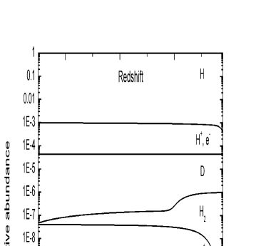
Figure 1: Fractional abundance of chemical species involved in the HD molecule formation as a function of redshift for the expanding and adiabatically cooling homogeneous primordial medium. The concordance $\Lambda$CDM cosmological model was used.

3 The HD optical depth in protohaloes and haloes at high redshifts

We are now interested in obtaining estimates related to the observability of the line features of the primordial HD molecule in protostructures in their linear or quasi–linear evolution regime, i.e. before gravitational collapse, and first star formation. As mentioned in the Introduction, previous works have shown that the largest resonant line opacities in homogeneous mass perturbations are produced when they are at their maximum expansion or turn–around epoch. Based on these conclusions, here we will calculate the HD resonant line opacities at the turnaround epoch of CDM high–peak mass perturbations. After the first bursts of star formation (Population III stars) in the high–peak ($3-6\sigma$) collapsed perturbations, re–ionization, feedback and metal enrichment processes change drastically the properties of the medium in the lower density mass perturbations. This is why we will focus on the protostructures emerging from high 3–6$\sigma$ peaks. The interaction of CMBR photons with the primordial molecules inside these protostructures will produce signatures related to the pristine conditions of gas before the first star formation in the universe.

3.1 Properties of 3 and $6\sigma$ top–hat CDM protohaloes and haloes

Table 1: Properties of $\Lambda$CDM mass perturbations

$M$	$z_{ta}$	$\rho_{ta}$	$n_{ta}$	$R_{ta}$	$z_{col}\hskip 4.2679pt$	$\rho_{col}$	$n_{col}$	$R_{col}$	$t_{dyn}\hskip 7.11317pt$	$z_{cool}\hskip 1.42262pt$	$n_{cool}$
$(M_{\odot})$		$(gcm^{-3})$	$(cm^{-3})$	$(cm)$		$(gcm^{-3})$	$(cm^{-3})$	$(cm)$	$(Myr)$		$(cm^{-3})$
Case $3\sigma$
$10^{2}$	58.52	3.02 $10^{-24}$	2.67 $10^{-1}$	2.50 $10^{19}$	36.49	2.40 $10^{-23}$	2.12 $10^{+0}$	1.26 $10^{19}$	13.58	32.65	2.12 $10^{3}$
$10^{4}$	46.26	1.51 $10^{-24}$	1.34 $10^{-1}$	1.46 $10^{20}$	28.77	1.20 $10^{-23}$	1.06 $10^{+0}$	7.34 $10^{19}$	19.20	25.72	1.06 $10^{3}$
$10^{6}$	34.55	6.44 $10^{-25}$	5.70 $10^{-2}$	9.03 $10^{20}$	21.40	5.11 $10^{-24}$	4.52 $10^{-1}$	4.53 $10^{20}$	29.43	19.10	4.52 $10^{2}$
$10^{8}$	24.17	2.28 $10^{-25}$	2.02 $10^{-2}$	5.92 $10^{21}$	14.85	1.81 $10^{-24}$	1.60 $10^{-1}$	2.97 $10^{21}$	49.40	13.23	1.60 $10^{2}$
$10^{10}$	15.18	6.07 $10^{-26}$	5.37 $10^{-3}$	4.28 $10^{22}$	9.19	4.82 $10^{-25}$	4.27 $10^{-2}$	2.14 $10^{22}$	95.78	8.15	4.27 $10^{1}$
$10^{12}$	7.92	1.02 $10^{-26}$	8.99 $10^{-4}$	3.60 $10^{23}$	4.61	8.10 $10^{-26}$	7.16 $10^{-3}$	1.80 $10^{23}$	233.69	4.03	7.16 $10^{0}$
Case $6\sigma$
$10^{2}$	118.04	2.42 $10^{-23}$	2.14 $10^{+0}$	1.25 $10^{19}$	73.99	1.92 $10^{-22}$	1.70 $10^{+1}$	6.28 $10^{18}$	4.80	66.30	1.70 $10^{4}$
$10^{4}$	93.53	1.21 $10^{-23}$	1.07 $10^{+0}$	7.32 $10^{19}$	58.55	9.60 $10^{-23}$	8.49 $10^{+0}$	3.67 $10^{19}$	6.79	52.45	8.49 $10^{3}$
$10^{6}$	70.10	5.15 $10^{-24}$	4.56 $10^{-1}$	4.52 $10^{20}$	43.79	4.08 $10^{-23}$	3.61 $10^{+0}$	2.26 $10^{20}$	10.40	39.20	3.61 $10^{3}$
$10^{8}$	49.34	1.83 $10^{-24}$	1.62 $10^{-1}$	2.96 $10^{21}$	30.71	1.45 $10^{-23}$	1.28 $10^{+0}$	1.48 $10^{21}$	17.47	27.46	1.28 $10^{3}$
$10^{10}$	31.37	4.86 $10^{-25}$	4.30 $10^{-2}$	2.14 $10^{22}$	19.39	3.86 $10^{-24}$	3.41 $10^{-1}$	1.07 $10^{22}$	33.86	17.30	3.41 $10^{2}$
$10^{12}$	16.86	8.16 $10^{-26}$	7.22 $10^{-3}$	1.80 $10^{23}$	10.25	6.48 $10^{-25}$	5.73 $10^{-2}$	9.02 $10^{22}$	82.62	9.10	5.73 $10^{1}$

To calculate the optical depth of primordial protoclouds by scattering of CMBR photons on HD molecules we need a model for these protoclouds. We use the spherical top–hat approach to calculate the epoch, density, and size of CDM mass perturbations at their maximum expansion for the $\Lambda$CDM cosmology adopted here. This approach is justified for the kind of estimates in which we are interested (e.g., Tegmark et al. 1997), and for the quasi–lineal phases of gravitational evolution. It is assumed that gas is equally distributed as CDM in the mass perturbation but with a density $\Omega_{B,0}/\Omega_{M,0}$ times lower. According to the spherical top–hat approach, the overdensity of a given mass perturbation, $\delta(M)$, grows with $z$ proportional to the so–called growing factor, $D(z)$, until it reaches a (linearly extrapolated) critical value, $\delta_{c}$, after which the perturbation is supposed to collapse and virialize at redshift $z_{\rm col}$ (for example see Padmanabhan 1993):

$$\delta(M;z_{\mathrm{col}})\equiv\delta_{0}(M)D(z_{\mathrm{col}})=\delta_{c,0}.$$ (12)

The convention is to fix all the quantities to their linearly extrapolated values at the present epoch (indicated by the subscript “0”) in such a way that $D(z=0)\equiv D_{0}=1$.

The redshift of turn–around, $z_{\mathrm{ta}}$, is calcualted by using the top–hat sphere result of $t_{\mathrm{ta}}=0.5t_{\mathrm{col}}$. Following the evolution equation for the top–hat sphere, one finds for our flat $\Lambda$CDM cosmology that the average sphere density at $z_{\mathrm{ta}}$ is given by $\rho_{\mathrm{ta}}\approx 5.6\rho_{\mathrm{bg}}(z_{\mathrm{ta}})$, i.e. similar to the Einstein–de Sitter case (Wang & Steinhardt 1998; Horellou & Berge 2005). The background density at $z_{\mathrm{ta}}$ is $\rho_{\mathrm{bg}}(z_{\mathrm{ta}})=1.88\ 10^{-29}$g cm${}^{-3}\Omega_{M,0}h^{2}(1+z_{\mathrm{ta}})^{3}$. The corresponding numerical gas density is $n_{\mathrm{ta}}=(\rho_{\mathrm{ta}}/m_{p})(\Omega_{B,0}/\Omega_{M,0})$, where $m_{p}$ is the H atom mass. Finally, the radius of the sphere of mass $M$ at the turn–around or maximum expansion is given by

$$R_{\mathrm{ta}}=\left[\frac{3M}{4\pi\rho_{\mathrm{ta}}}\right]^{\frac{1}{3}}.$$ (13)

We need now to connect the top–hat sphere results to a characteristic mass of the perturbation, $M$, produced within the $\Lambda$CDM structure formation scenario. The primordial fluctuation field, fixed at the present epoch, is characterized by the mass variance, $\sigma(M)$, which is the rms mass perturbation smoothed on a given scale $R$ corresponding to the mass $M$. For our calculations, we use the power spectrum shape given by Bardeen et al. (1986) normalized to $\sigma_{8}=0.9$. Thus, the mass perturbation overdensity linearly extrapolated to $z=0$ can be defined as:

$$\delta_{0}(M)=\nu\sigma(M),$$ (14)

where $M$ and $\nu$ are the perturbation mass and peak height, respectively. For average perturbations, $\nu=1$, while for rare, high–density perturbations, from which emerged the first structures, $\nu>>1$.

By introducing eq. (14) into eq. (12) one may infer $z_{\mathrm{col}}$, and therefore $z_{\mathrm{ta}}$, $\rho_{\mathrm{ta}}$, $n_{\mathrm{ta}}$, and $R_{\mathrm{ta}}$ for $\nu\sigma$ mass perturbations from the $\Lambda$CDM primordial fluctuation field. In Table 1 we present these quantities for $3\sigma$ perturbations of different masses. As mentioned above, we are interested in HD line signatures from the protoclouds before first luminous objects in the universe formed and started to re–ionize it, and therefore only high–peak low mass perturbations will be considered.

Cosmological N–body + hydrodynamics simulations showed that the first stars may have formed indeed at redshifts as high as $\sim 18-30$ in ($\sim 3-4\sigma$) CDM mini–haloes of M$\sim 10^{6}\mbox{M${}_{\odot}$}$ (Abell et al. 1998; 2002; Fuller & Couchman 2000; Bromm et al. 2002; Yoshida et al. 2003). Related to this is the fact that haloes of any given mass that collapse first (high peaks) do not populate “typical” regions at all, but rather “protocluster” regions (White & Springel 2000; Barkana & Loeb 2002). In a recent paper, Gao et al. (2005) used a novel technique to follow with unprecedentedly high resolution the growth of the most massive progenitor of a supercluster region from $z\approx 80$ to $z=0$. By using this simulation, Reed et al. (2005) have found that, when the mass of the progenitor halo is $\approx 2.4\ 10^{5}$h${}^{-1}\mbox{M${}_{\odot}$}$ at $z\approx 47$, it undergoes baryonic collapse via H₂ cooling, triggering star formation at this early epoch. Of course, this halo should emerge from a very rare fluctuation peak, $\nu=6.5$ (Reed et al. 2005). Notice that rare peaks are strongly clustered, so that the probability to find a cluster of these (proto)halos is high. In the second part of Table 1 we present the same as in the first part, but for $6\sigma$ haloes.

3.2 Optical depths

The optical depth for a protocloud of size $L$ is given by:

$$\tau_{\nu}\left(L\right)=\int_{0}^{L}\alpha_{\nu}\left(x\right)dx,$$ (15)

where $\alpha_{\nu}\left(x\right)$ is the absorption coefficient, and integration is carried out over the line of sight. In the case of a mass perturbation at its turn–around epoch, when the physical parameters of the gas are approximately equal for all parts of the spherical region, the integration can be reduced to a more simple expression: $\tau_{\nu}\left(L\right)\approx\alpha_{\nu}L$. So, the optical depth in this case can be written as:

$$\tau_{\nu}=\frac{\lambda^{3}\left(2J^{\prime}+1\right)}{8\pi\left(2J+1\right)V_{T}}x_{\mathrm{HD}}n_{\mathrm{J}}n_{B}A_{J^{{}^{\prime}}J}\left(1-e^{\frac{-h\nu}{\kappa T_{r}}}\right)L,$$ (16)

where $\lambda$ is the wavelength, $J$ is the rotational quantum number, $x_{\mathrm{HD}}$ is the relative abundance of the HD molecule, $A_{J^{{}^{\prime}}J}$ is the Einstein coefficient, and $n_{B}$ and $n_{\mathrm{J}}$ are the baryon and $J$–th rotational level population numerical densities at epoch $z$, respectively. As to $n_{J}\left(z\right)$, it is well known that at the low density limit ($n_{H}<10^{3}$cm^-3), the population differs from the Boltzmann one. So, in the general case, when the gas is out of thermodynamical equilibrium, the correct values of the ro–vibrational levels population should be calculated with the detailed balance equation:

$$n_{vJ}\sum_{v^{\prime}J^{\prime}}(W_{vJ\rightarrow v^{\prime}J^{\prime}}^{R}+W_{vJ\rightarrow v^{\prime}J^{\prime}}^{C})=$$ (17)

$$\sum_{v^{\prime}J^{\prime}}n_{v^{\prime}J^{\prime}}(W_{v^{\prime}J^{\prime}\rightarrow vJ}^{R}+W_{v^{\prime}J^{\prime}\rightarrow vJ}^{C}),$$ (18)

where $n_{vJ}$ is the population of the ro–vibrational level $vJ$, $W_{vJ\rightarrow v^{\prime}J^{\prime}}^{R}$ and $W_{vJ\rightarrow v^{\prime}J^{\prime}}^{C}$ are the probabilities of the radiative and collisional transitions, respectively.

By using the expressions (16) and (18), we calculate the HD line optical depths corresponding to protohaloes of several masses at their turnaround redshifts (Table 1). The results corresponding to three ground rotational line transitions (1–0), (2–1) and (3–2) for the $3\sigma$ and $6\sigma$ protohaloes are plotted in Figs. 2 and 3, respectively. As one can see, the values of the optical depth for the HD molecule lines are rather large as compared with those reported for the LiH molecule (Bougleux & Galli 1997). Even the transition $J^{\prime}-J=3-2$ reaches values as high as $10^{-9}-10^{-8}$ for the redshifts $z\approx 20-40$.

The estimates presented above correspond to the linear evolution phase of fluctuations. The calculation of chemical kinematics evolution of HD molecule during the gas cooling and collapse inside the virializing dark haloes is very difficult since it is linked to the thermal and hydrodynamical evolution. Under several assumptions and simplifications, Galli & Palla (2002) presented results of HD abundances after the gas cooling inside virialized CDM haloes constructed according to Tegmark et al. (1997). The result of Galli & Palla is that the HD relative fraction, $x_{HD}$, increases dramatically, approximately by a factor of 200, with respect to the initial one at the collapse epoch of the halo. In the following, we will use this result to get a rough estimate of the HD relative fraction in collapsed $\Lambda$CDM haloes and the corresponding $\tau_{\nu}$.

We have calculated above the evolution of the HD relative fraction, $x_{HD}$, in the homogeneous pregalactic medium. For a given mass fluctuation $\nu\sigma$, we have obtained $x_{\mathrm{HD}}$ at $z_{\mathrm{ta}}$. Let us assume that after the halo collapsed, at $z_{\mathrm{col}}$, $n_{HD}$ increased only proportionally to the halo density increasing. Therefore, $n_{\mathrm{HD}}(z_{\mathrm{col}})=n_{\mathrm{HD}}(z_{\mathrm{ta}})\times\rho_{\mathrm{col}}/\rho_{\mathrm{ta}}$. Then, we assume that the gas cools rapidly and falls to the halo center in a dynamical time,

$$t_{\mathrm{dyn}}\approx\frac{\pi/2}{\sqrt{2GM/R_{\mathrm{col}}^{3}}}$$ (19)

where $R_{\mathrm{col}}$ is the halo radius. Now, according to the Galli & Palla result, we assume that at the epoch when the gas cooled and collapsed, $z_{\mathrm{cool}}$, the HD relative fraction increased by a factor of $\sim 200$, i.e. $x_{\rm HD}(z_{\rm cool})\approx 200\ x_{\rm{HD}}(z_{\rm{col}})$. The collapsing factor of the gas is assumed to be 10, so that the number density increases by a factor of 1000. We further assume that the kinetic temperature of the cooled gas is equal to the CMBR radiation (see Fig. 10 in Galli & Palla). The populations corresponding to the main ground line transition ($J^{\prime}-J$)=(1–0) actually depend weakly on $T_{k}$. In Fig. 4 we show the HD ($J^{\prime}-J$)=(1–0) line transition optical depths corresponding to 3 and $6\sigma$ haloes of several masses at their “cooling” redshifts. The radii used to calculate $\tau_{\nu}$ were 1/10th of the corresponding halo radii $R_{\rm{col}}$. For the redshifts of interest, i.e. before massive star formation ($z\mathrel{\hbox to0.0pt{\lower 3.0pt\hbox{$\mathchar 536\relax$}\hss}\raise 2.0pt\hbox{$\mathchar 318\relax$}}20$), the optical depths of the lines are significantly high, with values from several times $10^{-2}$ to several times $10^{-5}$, up to $z\sim 50$.

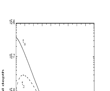
Figure 2: Optical depths in the first, second and third rotational transitions of HD molecule in $3\sigma$ $\Lambda$CDM protohaloes of different masses reaching their maximum expansion at the redshifts shown in the abscissa.

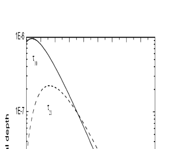
Figure 3: Same as in Fig. 2 but for $6\sigma$ $\Lambda$CDM protohaloes.

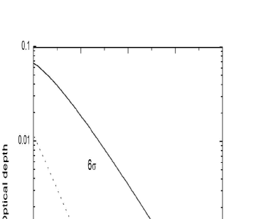
Figure 4: Same as in Figs. 2 and 3 but for haloes already collapsed and at the corresponding redshifts when the baryons have supposedly cooled and collapsed inside them (see text). Only the case for the first rotational transition is showed.

3.3 Observational estimates

As shown by Sunyaev & Zel’dovich (1970) (see also Dubrovich 1977; Zel’dovich 1978; Maoli et al. 1994) the amplitude of secondary anisotropies in the CMBR temperature due to Doppler effect of resonance scattered photons in protoclouds with peculiar motions is:

$$\frac{\Delta T}{T}=\frac{V_{p}}{c}\tau_{\nu}$$ (20)

for $\tau_{\nu}<<1$, where $V_{p}=V_{p}(z)$ is the peculiar velocity of the protocloud with respect to the CMBR at epoch $z$, $c$ is the light speed, and $\tau_{\nu}$ is the optical depth at frequency $\nu$ through the protocloud at epoch $z$ (to be the protocloud $z_{\mathrm{ta}}$ in our analysis). The linear theory of gravitational instability shows that the peculiar velocity of every mass element grows with the expansion factor as $V_{p}(z)\propto\dot{D}(z)/(1+z)$. An accurate approximation to this expression for a flat universe with cosmological constant is (Lahav et al. 1991; Carroll et al. 1992):

$$V_{p}(z)\propto f(z)\frac{g(z)}{g(0)}\frac{E(z)}{(1+z)^{2}},$$ (21)

where $f(z)\approx\Omega_{M}(z)^{0.6}$, and the functions $g(z)$, $E(z)$ and $\Omega_{M}(z)$ were defined in §3.1. For the Einstein–de Sitter universe, eq. (21) reduces to the known expression $V_{p}(z)\propto(1+z)^{-2}$.

The peculiar velocity field at $z=0$, traced by galaxies and galaxy clusters, has been measured in a large range of scales (for a review see e.g., Zaroubi 2002). For our problem, the velocity field traced by galaxy clusters is probably the interesting one because, as mentioned above, the first luminous objects in the universe formed in the densest, most rare regions, i.e. those that today are clusters of galaxies. Various data sets lead to different rms peculiar velocities for scales $\mathrel{\hbox to0.0pt{\lower 3.0pt\hbox{$\mathchar 536\relax$}\hss}\raise 2.0pt\hbox{$\mathchar 318\relax$}}100$h^-1Mpc. Here we will adopt a value of $V_{p}(0)\approx 650$km/s, in agreement with results from Lauer & Potsman (1994), Hudson et al. (1999,2004), and Willick (1999). This value is apparently a factor of $\sim 2$ larger than the one corresponding to $\Lambda$CDM numerical simulations for the scales of interest.

By using eq. (21) normalized to $V_{p}(0)=650$km/s and the HD optical depths calculated in §3.2, we may estimate with eq. (20) the corresponding temperature fluctuation of the secondary anisotropies. In the range of $z=20-40$, for the case of the $3\sigma$ protohaloes, we obtain that $\Delta T/T\approx\ 10^{-10}-4\ 10^{-12}$ in the first rotational transition, while for the $6\sigma$ protohaloes, $\Delta T/T\approx 5$ $10^{-10}-10^{-10}$. In the same redshift range, for the collapsed baryonic clouds, whose HD abundances were estimated using results from Galli & Palla (2002), we calculate $\Delta T/T\approx\ 10^{-6}-10^{-8}$ and $\Delta T/T\approx\ 2\ 10^{-5}-10^{-6}$ for the 3 and $6\sigma$ cases, respectively.

Now let us estimate the integration time required for the detection of the secondary anisotropies with millimeter and submillimeter facilities under construction as for example: the 50m LMT/GTM telescope in Sierra Negra, Mexico; the “Combined Array for Research in Millimeter–Wave Astronomy” (CARMA) in USA; the “Atacama Large Millimeter Array” (ALMA) in Chile. The observational (integration) time $\Delta t$ can be estimated from the equation

$$\Delta T=\frac{T_{n}}{\sqrt{\Delta\nu\Delta t}},$$ (22)

where $\Delta\nu$ is the bandwidth, $T_{n}$ is the detector noise temperature and $\Delta T$ is the amplitude of the temperature fluctuation calculated above. For the three facilities mentioned, $T_{n}\approx 40-80$ K, and we may assume $\Delta\nu\approx 1$. In the case of GTM/LMT telescope, its angular resolution limits the observability of several cases (see below). By using eq. (22), for the $3\sigma$ and $6\sigma$ protohaloes, we find that the integration times required to get an observable signal of the first rotational transition of HD molecules are too large to be observed. In the case of collapsed gas clouds (previous to star formation triggering) inside virialized $6\sigma$ haloes, we estimate $\Delta t\mathrel{\hbox to0.0pt{\lower 3.0pt\hbox{$\mathchar 536\relax$}\hss}\raise 2.0pt\hbox{$\mathchar 316\relax$}}10^{5}s=28\$ hours for $z<40$ and $T_{n}\approx 50$ K. This integration time can be attained at different observational sessions of several hours each.

Let us discuss another important parameter of the potentially observed protoclouds in molecular resonant line emission: their apparent angular size or diameter. Apparent angular size for an object of the linear size $L$ is given by the Hoyle’s formula:

$$\Delta\theta=\frac{L}{d_{A}(z)},$$ (23)

where $d_{A}(z)$ is the angular-diameter distance.

The angular–diameter distance for a flat universe with cosmological constant is given by:

$$d_{A}(z)=\frac{c}{\left(1+z\right)}\int_{0}^{z}\frac{dz^{\prime}}{H(z^{\prime})},$$ (24)

where the Hubble parameter in this case is:

$$H(z)=H_{0}\sqrt{\Omega_{M,0}(1+z)^{3}+\Omega_{\Lambda}},$$ (25)

and the radiation density term was neglected. Now eq. (23) can be written as follows:

$$\Delta\theta=\frac{H_{0}L(1+z)}{c\int_{0}^{Z}\left(\Omega_{M,0}(1+z^{\prime})^{3}+\Omega_{\Lambda}\right)^{-1/2}dz^{\prime}},$$ (26)

We use eq. (26) to calculate the angular size $\Delta\theta$ of $3$ and $6\sigma$ protoclouds reaching their maximum expansion in the redshift range of $20<z<40$ (corresponding roughly to mass ranges of $10^{5}<M/\mbox{M${}_{\odot}$}<10^{9}$ and $10^{9}<M/\mbox{M${}_{\odot}$}<10^{11}$ for the $3\sigma$ and $6\sigma$ cases, respectively). We calculate also the corresponding redshifted frequencies, $\nu_{0}$, for the same three lowest rotational transitions of HD molecule considered in Figs. 2 and 3. Our results are shown in Fig. 5, along with the expected coverage in this $\nu_{0}-\Delta\theta$ plane for the LMT/GTM and CARMA facilities (boxes). The ALMA facility covers the whole plotted plane. We also include in this plot the curves corresponding to the cold clouds within collapsed $3$ and $6\sigma$ haloes for only the first rotational transition line (thin lines with square dots). These clouds could be resolved by ALMA and only partially by CARMA. It should be noted that high–peak halos are strongly clustered (Gao et al. 2005; Reed et al. 2005). It may thus be more plausible to find a cluster of such objects in a patch of the sky even if individual objects are very small. Moreover, the clustering increases the amplitude of the spectra–spatial fluctuations in the CMBR temperature. Figure 5 is rather general and can be applied to any other resonant lines of similar frequencies in which the gas in protohaloes or haloes could be detected.

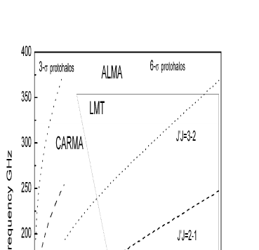
Figure 5: Relation between the angular size $\Delta\theta$ of the $3\sigma$ and $6\sigma$ protoclouds reaching their maximum expansion at $20<z<40$ and the redshifted frequency for three lowest rotational transitions of the HD molecule. Thin lines with squared dots are for $3\sigma$ (upper curve) and $6\sigma$ (lower curve) collapsed cold clouds in the same redshift range and only for the lowest transition. The boxes indicate qualitatively the regions in which the LMT/GTM and CARMA will operate. ALMA will cover almost the whole plotted plane.

4 Discussion and Conclusions

The hope to detect signals from the end of the so–called ’dark age’ has prompted a flurry of theoretical and instrumental activity. The observation of high–redshift protostructures before they collapse and star formation triggers will certainly help us to constrain structure formation scenarios. One possibility of such observations is based on the spectral–spatial fluctuations in the CMBR temperature produced by elastic resonant scattering of CMBR photons on molecules located in protostructures moving with peculiar velocity. This kind of secondary anisotropies search for LiH molecule has been fruitless (de Bernardis et al. 1993). As Bougleux & Galli (1997) showed, the abundances of LiH molecule and their optical depths in the rotational lines are too small to produce detectable CMBR temperature fluctuations.

In this paper we have investigated the spectral–spatial fluctuations in the the CMBR temperature due to elastic resonant scattering by HD molecules. For this molecule, the main contribution to the optical depth comes from the ground rotational transition ($J^{\prime}-J$)=(1–0), because of small populations with high rotational levels of the HD molecule at early epochs. In the case of the LiH molecule, most of the contribution to the optical depth comes from rotational transitions between high $J$ levels. The wavelenght at rest of the HD ($J^{\prime}-J$)=(1–0) transition is 112.1 $\mu m$. Therefore, for $z=20-40$ it should be observed at the wavelengths $\approx 2-4.5$mm. For higher rotational transitions, the wavelengths are smaller.

We have carried out calculations in order to estimate the HD optical depths and the corresponding amplitudes of the spectral–spatial fluctuations in the CMBR temperature produced by moving protostructures. First we calculated detailed chemical kinematic evolution for HD molecule in the expanding and adiabatically cooling homogeneous medium, assuming standard BBN yields. We further calculated the optical depths in HD pure rotational lines for mass perturbations (protostructures) at their maximum expansion under the assumption that the HD relative fractions, $x_{HD}$, within these protostructures are similar to the fractions calculated for the homogeneous medium at a given $z$. The spherical top–hat approach and the concordance $\Lambda$CDM cosmology were used to calculate the corresponding turn–around redshifts, sizes, and peculiar velocities for different masses and peaks. Once the optical depths for the first three ground rotational transitions were calculated, the corresponding fluctuations $\Delta T/T$ were estimated. We also estimated $\tau_{\nu}$ and $\Delta T/T$ for cold gas clouds inside collapsed CDM haloes, but under several assumptions and using results on the HD relative fraction from a crude calculation by Galli & Palla (2002).

The main results from our study are the following:

$\bullet$ The relative fraction of HD molecule, $x_{\rm HD}$, increases in the homogeneous expanding medium by a factor of $\approx 400$ since $z=300$ to low redshifts (Fig. 1). At redshifts $40-20$, $x_{\rm HD}\approx 4-5\ 10^{-10}$. These fractions are expected to strongly increase during the cooling and collapse of the gas within CDM haloes.

$\bullet$ The optical depth of the HD first pure rotational line in high–peak protostructures at their maximum expansion increases with time. For the second and third lines, the corresponding $\tau_{\nu}$’s attain a maximum at high redshifts and then strongly decrease for lower redshifts. The ranges of $\tau_{\nu}$ values of the (1–0) transition lines in 3 and $6\sigma$ protostructures at their maximum expansion in the $20<z<40$ redshift interval are approximately $10^{-7}-6\ 10^{-9}$ and $8\ 10^{-7}-2\ 10^{-7}$, respectively (Figs. 2 and 3). For the crude model of cold gas clouds inside collapsed 3 and $6\sigma$ CDM haloes, the ranges of $\tau_{\nu}$ in the same redshift interval are $8\ 10^{-4}-10^{-5}$ and $2\ 10^{-2}-1.3\ 10^{-3}$, respectively (Fig. 4). The optical depths of HD rotational lines in protostructures are much higher than those of the LiH molecule.

$\bullet$ The ranges of redshifted frequencies and typical angular sizes in the sky of spectral–spatial fluctuations due to HD molecule rotational lines in high–peak protostructures and gas clouds in collapsed haloes fall partially within the observational windows of submillimeter telescope facilities under construction, as GTM/LMT, CARMA and ALMA (Fig. 5). The range of redshifts under consideration was $20<z<40$; after this epoch the first baryonic structures are probably already in site with strong emitting stellar sources. The observational search of the spectral–spatial fluctuations studied here will be important for testing models of cosmic structure formation as well as the primordial abundance of deuterium predicted in standard and non-standard BBN theories.

$\bullet$ For the $\Lambda$CDM scenario, the amplitudes of the spectral–spatial fluctuations produced by HD molecule at $20<z<40$ in protostructures, even as rare as $3-6\sigma$ density–peaks, are too faint for reaching the flux sensitivity of submillimeter/millimeter facilities under construction. For the case of cold gas clouds within collapsed $\Lambda$CDM haloes emerging from $\sim 6\sigma$ density–peaks, the estimated amplitudes, in particular for the lowest rotational transition line, are much larger and could be detected, but their estimated angular sizes in the sky are too small for telescopes such as GTM/LMT, but possibly clusters of such objects could be resolved (high–peak halos are strongly clustered). The spectral–spatial fluctuations predicted for very rare high–redshift cold clouds in the $\Lambda$CDM scenario will fall within the observational capabilities of other facilities as CARMA and ALMA. For non-standard BBN theories, the [D/H] abundance can be much larger than the used here. For example, in inhomegeneous BBN models, [D/H] is estimated to be ten times larger than in the standard BBN (e.g., Lara 2005). Therefore the HD line optical depths presented here could be a factor of ten higher, making already detectable the corresponding spectral–spatial fluctuations produced at the maximum expansion of protohaloes.

A more detailed study of spectral–spatial fluctuations due to HD molecules in collapsing gas clouds as well as the inclusion of alternative BBN models is necessary in order to get more precise results and predictions than the ones presented here. In this paper we have carried out preliminary calculations that show the viability of using HD molecule lines to search for signatures of early structure formation in the universe and/or to constrain cosmological theories.

References

- Abel et al (1998) Abel T., Anninos P., Norman M., Zhang Y., 1998, ApJ, 508, 518
- Abgrall et al (1998) Abgrall H., Roueff E., Viala Y., 1982, A&AS, 50, 505
- Bardeen et al (1986) Bardeen J.M., Bond J.R., Kaiser N., Szalay A.S., 1986, ApJ, 304, 15
- Barkana & Loeb (2002) Barkana R., Loeb A., 2002, ApJ, 578, 1
- Barkana & Loeb (2005) Barkana R., Loeb A., 2005, MNRAS, 363, L36
- Bougleux & Galli (1997) Bougleux E., Galli D., 1997, MNRAS, 288, 638
- Bromm et al (2002) Bromm V., Copi P.S., Larson R.B., 2002, ApJ, 564, 23
- Bromm & Larson (2004) Bromm V., Larson R.B., 2004, ARAA, 42, 79
- Carroll et al (1992) Carroll S.M., Press W.H., Turner E.L., 1992, ARAA, 30, 499
- de Bernardis et al (1993) de Bernardis P. et al., 1993, A&A, 269, 1
- Dubrovich (1977) Dubrovich V.K., 1977, Sov. Astron. Lett., 3, 128
- Dubrovich (1983) Dubrovich V.K., 1983, Bull. Spec. Astrophys. Obs. North Caucasus, 13, 31
- Dubrovich (1993) Dubrovich V.K., 1993, Astronomy Letters, 19, 53
- Dubrovich (1997) Dubrovich V.K., 1997, A&A, 324, 27
- Flower et al (2000) Flower D.R., Le Bourlot J., Pineau des Forets G. and Roueff E., 2000, MNRAS, 314, 753
- Fuller & Couchman (2000) Fuller T.M., Couchman H.M.P., 2000, ApJ, 544, 6
- Galli & Palla (1998) Galli D., Palla F., 1998, A&A, 335, 403
- Galli & Palla (2002) Galli D., Palla F., 2002 Planetary and Space Science, 50, Issue 12-13, 1197
- Gao et al (2005) Gao L., White S.D.M., Jenkins A., Frenk C.S., Springel, V., 2005, MNRAS, 363, 379
- Hogan & Rees (1979) Hogan C.J., Rees M.J., 1979, MNRAS, 188, 791
- Horellou & Berge (2005) Horellou C., Berge J., 2005, MNRAS, 360, 1393
- Hudson et al (1999) Hudson M.J., Smith R.J, Lucey J.R., Schlegel D.J., Davis R.L., 1999, ApJ, 512, L79
- Hudson et al (2004) Hudson M.J., Smith R.J., Lucey J.R., Branchini E., 2004, MNRAS, 352, 61
- Johnson & Bromm (2006) Johnson J.L., Bromm V., 2006, MNRAS, 366, 247
- Kamaya & Silk (2003) Kamaya H., Silk J., 2003, MNRAS, 339, 1256
- Khlopov & Rubin (2004) Khlopov M. Yu., Rubin S.G., 2004, “Cosmological Pattern of Microphysics in the Inflationary Universe”, Kluwer Academic Publishers, Dordrecht
- Lara (2005) Lara J. F., 2005, Phys.Rev. D72, 023509
- Lahav et al (1991) Lahav O., Lilje, P.B., Primack J.R., Rees M.J., 1991, MNRAS, 251, 128
- Lauer & Potsman (1994) Lauer T.R., Potsman M., 1994, ApJ, 425, 418
- Lipovka et al (2005) Lipovka A., Núñez–López R., Avila Reese V., 2005, MNRAS, 361, 854
- Maoli et al (1994) Maoli R., Melchiorri F., Tosti D., 1994, ApJ, 425, 372
- Maoli et al (1996) Maoli R., Ferrucci V., Melchiorri F., Signore M., Tosti D., 1996, ApJ 457, 1
- Maoli et al (2004) Maoli R. et al, 2004, ESA SP-577, 293, preprint (astro-ph/0411641)
- Oh & Haiman (2003) Oh S.P., Haiman Z., 2003, MNRAS, 346, 456
- Padmanabhan (1993) Padmanabhan T., 1993, Structure Formation in the Universe. Cambridge University Press.
- Puy & Signore (2002) Puy D., Signore M., 2002, AIP Conf.Pro., 616, 346, astro-ph/0108512
- Reed et al (2005) Reed D.S., Bower R., Frenk C.S., Gao L., Jenkins A., Theuns T., White S.D.M., 2005, MNRAS, 363, 393
- Shchekinov (1986) Shchekinov Yu. 1986, SvAL, 12, 211
- Spergel et al (2003) Spergel D.N. et al., 2003, ApJSS, 148, 175
- Stancil et al (1996) Stancil P.C., Lepp S., Dalgarno A., 1996, ApJ, 458, 401
- Sunyaev & Zeldovich (1970) Sunyaev R.A., Zel’dovich Ya.B., 1970, Ap&SS, 7, 3
- Tegmark et al (1997) Tegmark M., Silk J., Rees M.J., Blanchard A., Abel T., Palla F., 1997, ApJ, 474, 1
- Varshalovich et al (2001) Varshalovich D.A., Ivanchik A.V., Petitjean P., Srianand R., Ledoux C., 2001, Astronomy Letters, 27, 683
- Wang & Steinhardt (1998) Wang L., Steinhardt P.J., 1998, ApJ, 508, 483
- White & Springel (2000) White S.D.M., Springel V., 2000, in “The First Stars”, FSProc.MPA/ESO, p. 327 (astro-ph/9911378)
- Willick (1999) Willick J.A., 1999, ApJ, 522, 647
- Yoshida et al (2003) Yoshida N., Abel T., Hernquist L., Sugiyama N., 2003, ApJ, 592, 645
- Yoshida (2006) Yoshida N., 2006, New Astronomy Reviews, 50, 19
- Zaroubi (2002) Zaroubi S., 2002, preprint (astro-ph/0206052)
- Zeldovich (1978) Zel’dovich Ya.B., 1978, SvA Lett., 4, 88