MACHOs in dark matter haloes

Abstract

Using eight dark matter haloes extracted from fully-self consistent cosmological $N$-body simulations, we perform microlensing experiments. A hypothetical observer is placed at a distance of 8.5 kpc from the centre of the halo measuring optical depths, event durations and event rates towards the direction of the Large Magellanic Cloud. We simulate 1600 microlensing experiments for each halo. Assuming that the whole halo consists of MACHOs, $f=1.0$, and a single MACHO mass is $m_{\rm M}=1.0$ ${\rm M_{\odot}}$, the simulations yield mean values of $\tau=4.7^{+5.0}_{-2.2}\times 10^{-7}$ and $\Gamma=1.6^{+1.3}_{-0.6}\times 10^{-6}$ events star^-1 yr^-1. We find that triaxiality and substructure can have major effects on the measured values so that $\tau$ and $\Gamma$ values of up to three times the mean can be found. If we fit our values of $\tau$ and $\Gamma$ to the MACHO collaboration observations (Alcock et al., 2000), we find $f=0.23^{+0.15}_{-0.13}$ and $m_{\rm M}=0.44^{+0.24}_{-0.16}$. Five out of the eight haloes under investigation produce $f$ and $m_{\rm M}$ values mainly concentrated within these bounds.

1 Introduction

Experiments such as MACHO (Alcock et al., 2000) and POINT-AGAPE (Calchi Novati et al., 2005) have detected microlensing events towards the Large Magellanic Cloud (LMC) and the M31, supporting the view that some fraction of the Milky Way dark halo may be comprised of massive astronomical compact halo objects (MACHOs). The fraction of the dark halo mass in MACHOs, as well as the nature of these lensing objects and their individual masses can be constrained to some extent by combining observations of microlensing events with analytical models of the dark halo (e.g. Kerins 1998; Alcock et al. 2000; Cardone et al. 2001). However, the real dark halo might not be as simple as in analytical models, which typically have spherical or azimuthal symmetry and, in particular, smoothly distributed matter. Cosmological simulations indicate that dark matter haloes are neither isotropic nor homogeneous but are rather triaxial (e.g. Warren et al. 1992) and contain a notable amount of substructure (e.g. Klypin et al. 1999). Even for the Milky Way it is still unclear if the enveloping dark matter halo has spherical or triaxial morphology: a detailed investigation of the tidal tail of the Sgr dwarf galaxy supports the notion of a nearly spherical Galactic potential (Ibata et al. 2001; Majewski et al. 2003) whereas that the data are also claimed to be consistent with a prolate or oblate halo (Helmi, 2004). The shape of the halo has an effect on the predicted number of microlenses along different lines-of-sight, for comparison with the results of microlensing experiments.

In this paper, we examine the effects of dark halo morphology and dark halo clumpiness on microlensing surveys conducted by hypothetical observers located in eight $N$-body dark matter haloes formed fully self-consistently in cosmological simulations of the concordance $\Lambda$CDM model. The eight haloes are scaled to approximately match the Milky Way’s dark halo in mass and rotation curve properties, and hypothetical observers are placed on the surface of a “Solar sphere” (i.e. 8.5 kpc from the dark halo’s centre) from where they conduct microlensing experiments along lines-of-sight simulating the Sun’s line-of-sight to the LMC. The effects on microlensing of triaxiality and clumping in the haloes are examined.

The paper expands upon work in a study by Widrow & Dubinski (1998) although we take a slightly different point of view. Instead of studying the errors caused by different analytical models fitted to an $N$-body halo, we analyse the microlensing survey properties of the simulated haloes directly. That is, we do not try to gauge the credibility of analytical microlensing descriptions but rather use our self-consistent haloes for the inverse problem in microlensing (Cardone et al., 2001). In other words, the free parameters (the MACHO mass and the fraction of matter in MACHOs) are determined from the observations via the optical depth, event duration and event rate predictions of the models. This not only allows us to make predictions for these parameters based upon fully self-consistent halo models but also to investigate the importance of shape and substructure content of the haloes.

The paper is structured as follows. We describe the $N$-body haloes and their preparation in Section 2, the simulation details are covered in Section 3, equations for the observables are derived in Section 4, results are given in Section 5, some discussion is presented in Section 6, final conclusions are in Section 7.

2 The Haloes

2.1 Cosmological simulation details

Our analysis is based on a suite of eight high-resolution $N$-body simulations (Gill, Knebe & Gibson, 2004a) carried out using the publicly available adaptive mesh refinement code MLAPM (Knebe, Green & Binney, 2001) in a standard $\Lambda$CDM cosmology ($\Omega_{0}=0.3,\Omega_{\lambda}=0.7,\Omega_{b}h^{2}=0.04,h=0.7,\sigma_{8}=0.9$). Each run focuses on the formation and evolution of galaxy cluster sized object containing of order one million collisionless, dark matter particles, with mass resolution $1.6\times 10^{8}$ $h^{-1}{\ }{\rm M_{\odot}}$ and force resolution $\sim$2$h^{-1}{\ }{\rm kpc}$ (of order 0.05% of the host’s virial radius). The simulations have sufficient resolution to follow the orbits of satellites within the very central regions of the host potential ($\geq$ 5–10 % of the virial radius) and the time resolution to resolve the satellite orbits with good accuracy (snapshots are stored with a temporal spacing of $\Delta t\approx$ 170 Myr). Such temporal resolution provides of order 10-20 timesteps per orbit per satellite galaxy, thus allowing these simulations to be used in a previous paper to accurately measure the orbital parameters of each individual satellite galaxy (Gill et al., 2004b).

The clusters were chosen to sample a variety of environments. We define the virial radius $R_{\rm vir}$ as the point where the density of the host (measured in terms of the cosmological background density $\rho_{b}$) drops below the virial overdensity $\Delta_{\rm vir}=340$. This choice for $\Delta_{\rm vir}$ is based upon the dissipationless spherical top-hat collapse model and is a function of both cosmological model and time. We further applied a lower mass cut for all the satellite galaxies of $1.6\times 10^{10}$ $h^{-1}{\ }{\rm M_{\odot}}$ (100 particles). Further specific details of the host haloes, such as masses, density profiles, triaxialities, environment and merger histories, can be found in Gill, Knebe & Gibson (2004a) and Gill et al. (2004b). Table LABEL:HaloDetails gives a summary of a number of relevant global properties of our halo sample. There is a prominent spread not only in the number of satellites with mass $M_{\rm sat}>1.6\times 10^{10}$$h^{-1}{\ }{\rm M_{\odot}}$ but also in age, reflecting the different dynamical states of the systems under consideration.

Table 1: Summary of the eight host dark matter haloes. The superscript $cl$ indicates that the values are for the unscaled clusters. Column 2 shows the virial radius, $R_{\rm vir}$; Column 3 the virial mass, $M_{\rm vir}$; Column 4 the redshift of formation, $z_{\rm form}$; Column 5 the age in Gyr; and the final column an estimate of the number of satellites (subhaloes) in each halo, $N_{\rm sat}$.

Halo	$R_{\rm vir}$cl	$M_{\rm vir}$cl	$z_{\rm form}$	age	$N_{\rm sat}$
	$h^{-1}{\ }{\rm Mpc}$	$10^{14}$ $h^{-1}{\ }{\rm M_{\odot}}$		Gyr
# 1	1.34	2.87	1.16	8.30	158
# 2	1.06	1.42	0.96	7.55	63
# 3	1.08	1.48	0.87	7.16	87
# 4	0.98	1.10	0.85	7.07	57
# 5	1.35	2.91	0.65	6.01	175
# 6	1.05	1.37	0.65	6.01	85
# 7	1.01	1.21	0.43	4.52	59
# 8	1.38	3.08	0.30	3.42	251

2.2 Downscaling

As we intend to perform microlensing experiments directly comparable to the results of the MACHO collaboration we need to scale our haloes to the size of the Milky Way. For this purpose we follow Helmi, White & Springel (2003) and apply an adjustment to the length scale, requiring that densities remain unchanged. Hence the scaling relations are:

$$r = \gamma r^{cl}$$ (1)

$$v = \gamma v^{cl}$$ (2)

$$m = \gamma^{3}m^{cl}$$ (3)

$$t = t^{cl}$$ (4)

where $r$ is any distance, $v$ is velocity, $m$ is mass, $t$ is time and the superscript $cl$ refers to the unscaled value. Because the haloes are downscaled, $\gamma$ will always be in the range $\gamma\in[0,1]$.

To find a suitable $\gamma$, the maximum circular velocity of each halo is required to be 220 km s^-1. The resulting (scaled) rotation curves for all eight haloes are shown in Figure 1. This figure highlights that Halo #8 is a special system — its evolution is dominated by the interaction of three merging haloes (Gill et al., 2004b). We do not consider Halo #8 to be an acceptable model of the Milky Way, but we include it into the analysis as an extreme case.

One might argue that our (initially) cluster sized objects should not be used as models for the Milky Way for they formed in a different kind of environment with less time to settle to (dynamical) equilibrium (i.e. the oldest of our systems is 8.3 Gyr vs. $\sim$ 12 Gyr for the Milky Way). However, Helmi, White & Springel (2003) showed that more than 90% of the total mass in the central region of a realistic Milky Way model was in place about 1.5 Gyr after the formation of the object. Our study focuses exclusively on this central region (i.e. the inner 15% in radius) boosting our confidence that our haloes do serve as credible models of the Milky Way for our purposes.

In Table LABEL:ScaledHaloes we list the scaled radii and masses, as well as the scaling factor $\gamma$, for each halo. Note that we have adopted a Hubble constant of $h=0.7$, which applies throughout the paper. The circular velocity (rotation) curves for the scaled haloes are shown in Figure 1 and demonstrate how the scaled mass $M(<r)$ is accumulated out to 400 kpc. Two vertical lines mark the position of observers at the Solar circle and the distance of the LMC from the halo centre; within this region, we note that the mass profiles are similar in all haloes, however, there are differences, especially for halo #8 (the dynamically merging system of haloes).

Table 2: Properties of the haloes after downscaling to Milky Way size. Column 2 shows the scale factor for each halo, $\gamma$; Column 3 shows the scaled virial radius, $R_{\rm vir}$; Column 4 the scaled virial mass, $M_{\rm vir}$; and the final column the scaled particle mass, $m_{p}$.

Halo	$\gamma$	$R_{\rm vir}$	$M_{\rm vir}$	$m_{p}$
		kpc	$10^{12}$ M⊙	$10^{6}$ M⊙
#1	0.197	380	3.08	1.75
#2	0.248	378	3.00	3.47
#3	0.253	391	3.39	3.71
#4	0.277	388	3.23	4.86
#5	0.197	383	3.14	1.76
#6	0.267	402	3.61	4.33
#7	0.278	403	3.67	4.92
#8	0.213	421	4.19	2.21

Figure 1: Circular velocity curves of the downscaled haloes ($V_{c}=\sqrt{GM(r)/r}$). Note that the maximum of each curve is at 220 km s^-1. The scaling factors $\gamma$ are shown in Table LABEL:ScaledHaloes. The two vertical lines at 8.5 kpc and 50.1 kpc mark the distances of the Sun and the LMC from the centre of the Milky Way.

2.3 Characteristics

Dark matter haloes within cosmological simulations are very different from the idealised analytical dark haloes that are described by only a few parameters. Two significant characteristics of the dark haloes that are not captured by the analytical models are triaxialty and substructure. For example, within the simulations on both cluster and galactic scales, the dark matter haloes are triaxial rather than spherical (Warren et al. 1992, Jing & Suto 2002). However, when gas dynamics is included within the simulation, these clusters/galaxies are more spherical (Katz & Gunn 1991, Evrard et al. 1994, Dubinski 1994), and when cooling is included within the simulation, the haloes are even more spherical (Kazantzidis et al., 2004).

Simulations show that CDM haloes contain a large number of subhaloes at both galactic and cluster scales (i.e. satellites) (Klypin et al. 1999, Moore et al. 1999), further Moore et al. (1999) assert that galaxy haloes appear as scaled versions of galaxy clusters with respects to the subhalo populations.

However, within the inner regions of the host haloes (on both galactic and cluster scales) the number density of subhaloes decreases considerably (Ghigna et al. 2000, Gill et al. 2004b, Diemand, Moore, & Stadel 2004). Even though these results seem to hold under numerical convergence tests (Diemand, Moore, & Stadel, 2004), the dynamical properties of the dark matter subhaloes differ from the observed galaxies within clusters.

With the use of semi-analytical techniques these differences have been accounted for (Gao et al. 2004; Taylor & Babul 2004). Gao et al. (2004) conclude that the tidal stripping of the dark haloes was very efficient in reducing the dark matter mass of the subhaloes while having less of an effect on the tightly bound baryonic galaxy at its core. Thus, while the dark matter subhaloes in the inner regions were being disrupted, baryonic cores survived.

For our pure dark matter simulations (Gill et al., 2004b) we also see this lack of dark matter substructure in the inner regions. This is shown in Table LABEL:Nsat, where we list the subhaloes (along with some of their (downscaled) integral properties) found in the inner 70 kpc of each halo. Note that masses of the subhaloes are limited to a relevant range, $5.0\times 10^{8}$ ${\rm M_{\odot}}$$<M_{\rm sat}<1.0\times 10^{10}$ ${\rm M_{\odot}}$.

For the Milky Way, we know that at least one large satellite exists within the inner 70 kpc: the LMC. Thus, whatever the paucity of satellites in inner regions of dark haloes in the simulations, here at least is one real-world example. The mass of the LMC is estimated to be $M_{\rm LMC}(8.9{\rm\leavevmode\nobreak\ kpc})=8.7\pm 4.3\times 10^{9}$ ${\rm M_{\odot}}$ from kinematical data (Marel et al., 2002). Reassuringly enough, we do find a few satellites with similar masses (cf. Table LABEL:Nsat) in the simulated haloes. Whether there are more (dark) satellites in the inner regions of the Milky Way than in our models is an open question.

Table 3: Substructure within the inner 70 kpc of the (downscaled) haloes. Column 1 shows the name of the halo; Column 2 the distance from the centre of the subhalo to the centre of the host, $l_{\rm sat}$; Column 3 the truncation radius of the subhalo (within the truncation radius, the density of the subhalo is larger than the background density of the host halo) , $r_{\rm sat}$; Column 4 the number of bound particles in the subhalo, $N_{\rm sat}$; and the final column the mass of the subhalo, $M_{\rm sat}$.

Halo	$l_{\rm sat}$	$r_{\rm sat}$	$N_{\rm sat}$	$M_{\rm sat}$
	kpc	kpc	particles	$10^{9}$${\rm M_{\odot}}$
#1	67.0	34.6	1232	2.20
#1	20.0	45.4	2957	5.27
#1	23.5	27.9	632	1.13
#2	53.5	24.1	207	0.73
#2	44.8	23.3	186	0.66
#3	60.7	38.1	793	2.99
#3	63.0	32.7	466	1.76
#4	67.8	30.8	317	1.57
#7	38.5	48.7	1217	6.09
#7	62.4	22.6	124	0.62
#8	46.1	32.9	859	1.93

3 Setting the Stage

3.1 The microlensing cone

A Galactocentric coordinate system is given by the three eigenvectors of the inertia tensor of the respective halo. We choose the $z$-axis to coincide with the major axis. To conduct our microlensing experiments, we then place an observer at the Solar distance from the centre of a halo. There are various options for possible orientations with respect to the coordinate system; we basically restrict ourselves to the scenario where the observer is placed somewhere on a sphere of radius 8.5 kpc.

We sample the halo with a number of sightlines and combine the individual results obtained from these independent measurements to obtain values of interest. Once we put down an observer, we can construct an observational cone towards a region simulating observations of an LMC sized patch of sky, and compute the microlensing signal generated by particles in the cone out to a distance of 50.1 kpc (see Figure 2). The hypothetical LMC has also to be located in a realistic direction in respect to the observer.

We use 40 observers uniformly distributed on a sphere of radius $8.5$ kpc. Each observer observes 40 uniformly separated LMCs, for which the angle $(\vec{r}_{\rm obs},\leavevmode\nobreak\ \vec{r}_{LMC}-\vec{r}_{\rm obs})$ is kept fixed at 89.1^∘ (the original angle between $(\vec{r}_{\odot},\leavevmode\nobreak\ \vec{r}_{LMC}-\vec{r}_{\odot})$ in Galactocentric coordinates). This configuration (illustrated in Figure 3) gives 1600 individual sightlines, and microlensing cones, which sample different sets of particles within a halo. The choice for the number of sightlines is a compromise between computation time and sampling density. As seen in Figure 3, 1600 sightlines sample the volume quite sufficiently, even when the sightlines are drawn as lines instead of actual cones.

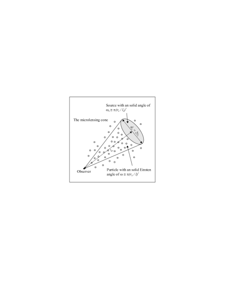
Figure 2: The microlensing sightline is defined by the locations of the observer and the source and the cone by the sightline and the source diameter. We use $l_{S}=50.1$ kpc and $d_{S}=4.52$ kpc. The particles inside the cone are treated as gravitational lenses. Typically $\sim$ 100 particles from the cosmological simulation are found inside a cone. This number is increased to $\sim$ 10000 by breaking them up into subparticles according to the recipe outlined in Section 3.2.

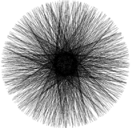
Figure 3: Sightlines used in the microlensing simulation. The image shows all 1600 sightlines of the 40 observers. The observers are located on a sphere with a radius of $r_{\odot}=8.5$ kpc. The sphere can be seen as the “dark ball” in the centre of the sightlines. The radius of the sphere which holds the sources is 49.5 kpc. Every observer has 40 sources (LMCs) at a distance of 50.1 kpc. The sightlines are not uniformly distributed because there is a limited number of observers and the angle $(\vec{r}_{\rm obs},\leavevmode\nobreak\ \vec{r}_{LMC}-\vec{r}_{\rm obs})$ is kept fixed at 89.1^∘. This is the original angle between $(\vec{r}_{\odot},\leavevmode\nobreak\ \vec{r}_{LMC}-\vec{r}_{\odot})$ in Galactocentric coordinates.

The microlensing cone itself is defined by the observer and the source. Figure 2 illustrates that we treat the source (i.e. LMC) as a circular disk with diameter $d_{S}$. The particles inside the cone are considered to be gravitational lenses. However, this kind of setup can lead to a handful of particles (those closest to the observer) contributing most to the optical depth. This leads to high sampling noise, and is essentially due to the limited resolution of the cosmological simulation (see Figure 4). It follows that the particle distribution has to be smoothed in some manner to suppress this noise; we describe this and the related issue of the MACHO masses in the next section.

3.2 Mass resolution vs. MACHO mass

In order to compute microlensing optical depths and other properties from the particles in the simulations, we need to get from a mass scale of order $10^{6}$ ${\rm M_{\odot}}$, i.e. that of the particles in the simulation, down to the mass scale of the MACHOS, of order 1 ${\rm M_{\odot}}$; i.e. we account for the fact that a typical particle in the simulations represents of order $10^{6}$ MACHOs.

To overcome the limitation imposed by the mass resolution of the simulation we recall that individual particles in the simulation are not treated as $\delta$-functions but have a finite size. The extent of a particle (i.e. its size) is determined — in our case — by the spacing of the grid, as we are using an adaptive mesh refinement code (i.e. MLAPM). In MLAPM the mass of each particle is assigned to the grid via the so-called triangular-shaped cloud (TSC) mass-assignment scheme (Hockney & Eastwood, 1981) which spreads every individual particle mass over the host and surrounding $3^{3}-1$ cells. The corresponding particle shape (in 1D) reads as follows:

$$S(x)=\left\{\begin{array}[]{ll}\displaystyle 1-\frac{|x|}{L}&\mbox{for $|x|<L$}\\ 0&\mbox{otherwise}\end{array}\right.$$ (5)

where $L$ is the spacing of the grid and $x$ measures the distance to the centre of the cell.

For each particle present in and around a particular cone along an observer’s line-of-sight, we determine the size of the finest grid surrounding it, which in turn determines the physical extent of the particle. The particle is then re-sampled with 100 “subparticles” whose positions are randomly chosen under the density distribution given by Equation 5. Figure 5 illustrates these “subparticle clouds”, sampled according to this TSC mass-assignment.

The improvement gained by using this method can be viewed in Figure 4 where we show measured optical depths (to be defined in Section 4.2) in a series of microlensing cones towards the LMC for observers continuously rotated on the edge of a disc perpendicular to the major axis of the dark halo. What is shown here is the noisy “original” estimates of optical depth for many lines-of-sight, compared to the optical depth measurements obtained when the particles within the cones have been resampled to “subparticles”. In the un-resampled case, the handful of particles which happen to reside close to the observer are found to dominate the calculation of the optical depth and other quantities of interest such as event duration and event rate. Variations in the optical depth from sightline to sightline can vary by up to a factor of three in the un-resampled sample cones, simply because a handful of particles dominate the microlensing. Convergence experiments have shown that breaking the original simulation particles down to 100 subparticles is sufficient to reduce the noise from this source to be negligible; if we were to use more subparticles, there is no further gain in accuracy.

Figure 4: Comparison between the use of cosmological simulation particles and triangular-shaped clouds containing 100 subparticles. For the illustration, we distributed 132 observers on a perimeter of a disk with a radius of 8.5 kpc, located on the $xy$-plane. The volumes of consecutive cones overlap by half. Without any resolution enhancements the variation in optical depth from cone to cone can be as large as a factor of three! This is due to the insufficient mass resolution of the cosmological simulation. We reached the Poissonian noise level, in which cone-to-cone variations are $<20$ %, with 100 subparticles, by experimenting. The large scale trend is due to triaxiality of the halo.

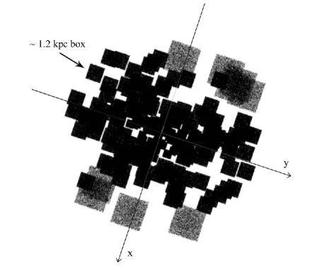
Figure 5: For this illustrative example of the subparticle clouds, we placed 222 cosmological simulation particles onto the $xy$-plane and broke each particle down to 10,000 subparticles. To get the subparticle positions, we used the triangular-shaped cloud density profile identically to the actual cosmological simulation. The subparticles form a cube (of a size of the corresponding MLAPM grid cell) around the position of the cosmological simulation particle. In the real microlensing simulation, the whole volume under investigation is filled with intersecting cubes and the void areas between the cubes seen here are not present.

The subparticles introduced have masses of order 10⁴ M_⊙, so we are unfortunately still orders of magnitudes away from actual MACHO masses. In the formulae introduced later (Section 4), each subparticle is expressed as a singular concentration of MACHOs. That is, a subparticle is treated as a set of MACHOs which have the same position and velocity as the subparticle itself, and for convenience in the simulations the MACHO mass is chosen to be $m_{\rm M}=1.0$ ${\rm M_{\odot}}$(although this is later relaxed by scaling). Figure 6 demonstrates the hierarchy of particles starting from the cosmological simulation particle down to the individual MACHOs.

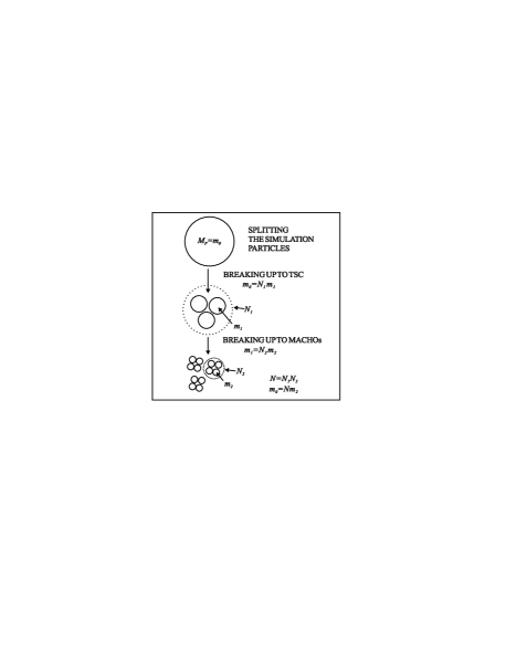
Figure 6: Splitting the cosmological simulation particle to 100 subparticles and a subparticle to $N_{\rm M}$ MACHOs. In the first phase, we break the cosmological simulation particle to 100 subparticles. The resulting subparticle represents an order of $N_{\rm M}\sim 10^{4}$ MACHOs with a mass of 1 M_⊙. The subparticle is treated as a MACHO concentration where the represented MACHOs all have a single location ($l_{\rm M}\equiv l_{\rm sub}$), mass ($m_{\rm M}\equiv m_{\rm sub}/N_{\rm M}$) and velocity ($v_{\rm M}\equiv v_{\rm sub}$).

4 The Microlensing Experiments

4.1 Definitions

Before going to the microlensing equations, we define what we mean by certain terms:

A microlensing source is a circular region, oriented perpendicularly to the line-of-sight of the observer, in which uniformly distributed background source stars are located. Because of the statistical nature of the source model, the number of background stars affects only the microlensing event rate. The region with a diameter $d_{S}$ and a distance $l_{S}$, is shown in Figure 2.

A source star is a star located somewhere in the disk of the microlensing source.

A microlens is also a circular region, oriented perpendicularly to the line-of-sight of the observer and centered on a dark particle. The region has a radius $r_{\rm E}$, which depends on the location and mass of the particle. Lenses are always inside a microlensing cone between the source and the observer.

A microlensing event is a detectable amplification of a source star caused by a microlens. Detectable means that the light of a source star is amplified by a factor larger than 1.34. This occurs when the sightline to a source star passes a particle within the lens radius, also known as the Einstein radius.

4.2 Optical depth

The Einstein radius $r_{\rm E}$ of a gravitational lens is defined as

$$r_{\rm E}^{2}=\frac{4Gm}{c^{2}}l^{2}\biggr{(}\frac{1}{l}-\frac{1}{l_{S}}\biggr{)}=Aml^{2}\biggr{(}\frac{1}{l}-\frac{1}{l_{S}}\biggr{)},$$ (6)

where $m$ is the mass of the lens, $l$ is the distance to the lens, $l_{S}$ is the distance to the source and $A=\frac{4G}{c^{2}}$.

For a single subparticle, we define the lens radius as

$$r_{\rm sub}^{2}=Am_{\rm sub}l_{\rm sub}^{2}\biggr{(}\frac{1}{l_{\rm sub}}-\frac{1}{l_{S}}\biggr{)},$$ (7)

where $m_{\rm sub}$ is the mass of the subparticle and $l_{\rm sub}$ the distance between the subpartice and the observer. Note that all subparticles within a halo have the same mass.

The optical depth of a single lens describes the probability that any given source star is amplified by the lens at any given time. Thus, the general equation for the optical depth of a lens can be written as the ratio of the solid angles of the lens and the source

$$\tau=\frac{\omega}{\omega_{S}},$$ (8)

where $\omega$ is the solid Einstein angle of the lens and $\omega_{S}$ is the solid angle of the source. When the solid angles are small, this can be approximated to

$$\tau\simeq\biggr{(}\frac{r_{\rm E}}{l}\frac{l_{S}}{r_{S}}\biggr{)}^{2}=Am\Theta^{-2}\biggr{(}\frac{1}{l}-\frac{1}{l_{S}}\biggr{)},$$ (9)

where $r_{S}$ is the radius of the source and $\Theta^{-2}=(l_{S}/r_{S})^{2}$. Note that $\Theta$ is approximately the half opening angle of the cone.

The optical depth of a subparticle with a mass $m_{\rm sub}$ is defined as

$$\tau_{\rm sub}=A\Theta^{-2}m_{\rm sub}\biggr{(}\frac{1}{l_{\rm sub}}-\frac{1}{l_{S}}\biggr{)}.$$ (10)

We take this value to be the total optical depth from all the $\sim 10^{4}$ MACHOs the subparticle represents.

Optical depth is additive, as long as the lenses do not overlap or cover the whole source, and so the total optical depth in a microlensing cone which contains $N$ subparticles is

$$\tau_{\rm cone}=\sum_{i}^{N}\tau_{\rm sub}^{(i)}=A\Theta^{-2}m_{\rm sub}\sum_{i}^{N}\biggr{(}\frac{1}{l_{\rm sub}^{(i)}}-\frac{1}{l_{S}}\biggr{)}$$ (11)

From Equation 11 it follows that the optical depth in a cone depends mainly on the distances of the subparticles related to the observer. The closer the particles are the larger is the optical depth. Section 3.2 covered the details of particle breaking, which also has a large effect on $\tau_{\rm cone}$. Note that $\tau_{\rm cone}$ does not depend on the MACHO mass $m_{\rm M}$.

4.3 Event duration

The event duration of a lens describes the typical duration of the amplifying event the lens would produce. The detected event durations in the MACHO experiment are the order of 100 days. Event duration depends on the tangential velocity with which a lens would seem to pass a source star and on the Einstein radius of the lens. The equation for an individual subparticle is

$$t_{\rm sub}=\frac{\pi}{2}\frac{r_{\rm sub}}{v_{\rm sub}},$$ (12)

where $r_{\rm sub}$ is the lens radius of the subparticle and $v_{\rm sub}$ the apparent tangential velocity difference between the subparticle and the source, respective to the observer.

The term $\frac{\pi}{2}$ is the average crossing length of a circle with an unit radius. By adding this term, we correct the event duration from the maximum value ($2r_{\rm E}/v$) to the statistically expected value. The correction can also be seen in the observational optical depth, $\tau_{meas}$, as a $\pi/4$ term in Eq. 1 of Alcock et al. (2000).

Using Equation 7, Equation 12 becomes

$$t_{\rm sub}=\frac{\pi}{2}m_{\rm sub}^{1/2}\frac{l_{\rm sub}}{v_{\rm sub}}\biggr{[}A\biggr{(}\frac{1}{l_{\rm sub}}-\frac{1}{l_{S}}\biggr{)}\biggr{]}^{1/2}.$$ (13)

However, this is not yet the value we are after. We need to solve $\hat{t}_{\rm sub}$, which is the average event duration caused by the subparticle’s MACHOs. To get $\hat{t}_{\rm sub}$, we simply replace $m_{\rm sub}$ with $m_{\rm M}$ and assign $l_{\rm M}\equiv l_{\rm sub}$ and $v_{\rm M}\equiv v_{\rm sub}$. We get

$$\hat{t}_{\rm sub}\equiv t_{\rm M}\equiv\frac{\pi}{2}m_{\rm M}^{1/2}\frac{l_{\rm sub}}{v_{\rm sub}}\biggr{[}A\biggr{(}\frac{1}{l_{\rm sub}}-\frac{1}{l_{S}}\biggr{)}\biggr{]}^{1/2},$$ (14)

where $t_{\rm M}$ is the event duration of a single MACHO when the MACHO inherits the location and the velocity of the subparticle. What is essentially stated in Equation 14 is that we use the event duration of a single MACHO as the average event duration for the whole subparticle.

As is well known, Equation 13 shows that, unlike the optical depth, event duration is a function of the MACHO mass. This fact can be used to find a preferred MACHO mass for a given event duration.

4.4 Event rate

Event rate $\Gamma$ for a given experiment is simply the number of expected events per an observing period for a given source. For a single lens it can be given as $\Gamma=\tau/t$, i.e., as the ratio of the optical depth and event duration.

The MACHO collaboration observed $\sim$ 13 - 17 events in 5.7 years. Usually, $\Gamma$ is given in events star^-1 yr^-1. The MACHO collaboration had $10.7\times 10^{6}$ source stars which gives (a maximum) of $\Gamma=17/5.7/(10.7\times 10^{6})$ events star^-1 yr${}^{-1}=2.79\times 10^{-7}$ events star^-1 yr^-1.

We calculate the event rate for a subparticle consisting of $N_{\rm M}$ MACHOs as

$$\Gamma_{\rm sub}=N_{\rm M}\Gamma_{\rm M}=N_{\rm M}\frac{\tau_{\rm M}}{t_{\rm M}}=N_{\rm M}\frac{\tau_{\rm sub}/N_{\rm M}}{\hat{t}_{\rm sub}}=\frac{\tau_{\rm sub}}{\hat{t}_{\rm sub}},$$ (15)

where $\Gamma_{\rm M}=\frac{\tau_{\rm M}}{t_{\rm M}}$ is the event rate for a single MACHO. By using Equations 10 and 13, the last term of Equation 15 expands to

$$\Gamma_{\rm sub}=\frac{2}{\pi}A^{1/2}\Theta^{-2}m_{\rm M}^{-1/2}m_{\rm sub}\frac{v_{\rm sub}}{l_{\rm sub}}\biggr{(}\frac{1}{l_{\rm sub}}-\frac{1}{l_{S}}\biggr{)}^{1/2}.$$ (16)

For the cone, we simply sum the event rates of the subparticles together, as was done to the optical depths in Equation 11

$$\Gamma_{\rm cone}=\frac{2}{\pi}A^{1/2}\Theta^{-2}m_{\rm M}^{-1/2}m_{\rm sub}\sum_{i}^{N}\frac{v_{\rm sub}^{(i)}}{l_{\rm sub}^{(i)}}\biggr{(}\frac{1}{l_{\rm sub}^{(i)}}-\frac{1}{l_{S}}\biggr{)}^{1/2}.$$ (17)

Note that $\Gamma_{\rm sub}\propto m_{\rm M}^{-1/2}$ whereas $\hat{t}_{\rm sub}\propto m_{\rm M}^{1/2}$.

5 Results

5.1 Differential optical depths and event rates

The results of our simulations are compared to the observations via the event duration because this is the only directly observed quantity. Our aim is to determine how optical depth $\tau$ and event rate $\Gamma$ depend on event duration.

In Figure 9, we show $d\tau/d\hat{t}$ and $d\Gamma/d\hat{t}$, averaged over all the 1600 cones for each halo, i.e we show for each simulated halo the global behaviour of differential optical depths and event rates as a function of event duration. The normalised standard deviations in these quantities amongst sightlines are shown (in separate panels, for clarity). Both curves for $\tau$ and $\Gamma$ peak in the range 50 and 100 days. This was expected as it is the result obtained from analytical models (e.g. Kerins 1998). Our simulations and the analytical results are in this sense adequate fits to the actual observations, in which the (few) events cluster around 100 days duration.

In Table LABEL:ResTab, we list the modal values for the distributions, $\hat{t}_{\rm exp}$, and the averaged cone values, $\langle\tau_{\rm cone}\rangle$ and $\langle\Gamma_{\rm cone}\rangle$, which are numerically integrated values of the differential functions in Figure 9. Note that the error limits on the last row (labelled “mean”) are simple mean values of the error limits from the corresponding column because they represent the mean variations between cones in a halo, not variations between haloes.

It can be seen that the integrated values differ between haloes. One might argue that there is a trend towards lower values from Halo #1 to Halo #8, and this is perhaps no surprise because the haloes were ordered by their dynamical age. Similar grouping of curves can be seen in the circular velocity profiles in Figure 1. Because circular velocity profiles reflect density profiles, it is the differences in matter densities between haloes that can be seen to cause differences in the integrated values of $d\tau/d\hat{t}$ and $d\Gamma/d\hat{t}$.

We have applied the MACHO collaboration efficiency functions to our simulations in order to get an idea of how their efficiency affects the overall observables. The results can be seen in Tables LABEL:ResTabA and LABEL:ResTabB. The efficiency functions reduce $\langle\tau_{\rm cone}\rangle$ and $\langle\Gamma_{\rm cone}\rangle$ by more than a factor of two and shift the expected event durations to be longer.

Note that all the following results are given in terms MACHO’s efficiency function “A” — this is the more conservative option of two efficiency functions given by the MACHO collaboration; tests show that both give very similar results.

Table 4: The mean optical depths and event rates, with their standard deviations, over the 1600 cones for each halo. See Figure 9 for the corresponding (differential) distribution functions — the numbers represented here are the integrated values of those functions. We also list the modes of the distributions: $\hat{t}_{\rm exp}$ columns give the most probable event duration for the respective distribution. Error limits show the variations between cones (i.e. microlensing experiments) in a halo.

Halo	$\langle\tau_{\rm cone}\rangle$	$\hat{t}_{\rm exp}$	$\langle\Gamma_{\rm cone}\rangle$	$\hat{t}_{\rm exp}$
	$10^{-7}$	days	$10^{-6}$	days
			events
			star-1 yr-1
#1	$5.6^{+6.0}_{-2.7}$	84	$2.0^{+1.7}_{-0.8}$	66
#2	$5.9^{+7.5}_{-2.7}$	74	$2.1^{+2.1}_{-0.8}$	64
#3	$4.3^{+3.8}_{-1.8}$	84	$1.4^{+1.1}_{-0.5}$	64
#4	$5.1^{+5.6}_{-2.4}$	86	$1.6^{+1.3}_{-0.7}$	64
#5	$4.1^{+3.4}_{-2.2}$	91	$1.3^{+0.9}_{-0.6}$	69
#6	$5.0^{+4.9}_{-1.9}$	81	$1.7^{+1.3}_{-0.6}$	71
#7	$4.7^{+6.6}_{-2.5}$	84	$1.6^{+1.6}_{-0.7}$	61
#8	$2.6^{+2.1}_{-1.0}$	104	$0.8^{+0.6}_{-0.3}$	81
mean	$4.7^{+5.0}_{-2.1}$	86	$1.6^{+1.3}_{-0.6}$	68

5.2 Substructure

An interesting feature can be seen in the relative standard deviation (i.e. normalised to the global mean) in Figure 9 of both $d\tau/d\hat{t}$ and $d\Gamma/d\hat{t}$ for Halo #1. The relative standard deviation of both functions has a peak around $\hat{t}=50$ days of greater than $1.0$ compared to typical values of $\sim$ 0.7. This peak is due to a subhalo with a mass of $5.27\times 10^{9}$ ${\rm M_{\odot}}$, i.e. the second subhalo of Halo #1 listed in Table 3. It is the only satellite with a substantial mass, concentration and location to cause any features to the $\tau$ and $\Gamma$ distributions. For example, Halo #7 contains a subhalo with a comparable mass ($6.09\times 10^{9}$ ${\rm M_{\odot}}$), but because it is located further away from the centre of the halo (and from the observer), it fails to affect the overall $\tau$ and $\Gamma$ distributions. The subhalo in Halo #1 is therefore the only substructure which could be directly associated with microlensing signal not associated with the global properties of the haloes.

It should be emphasized that the distributions shown in Figure 9 are averaged over all cones. The subhaloes, if present in a halo, contribute only to a small number of the cones and thus, possibly peculiar distributions are lost by the averaging process. In another words, the distribution functions of a single cone can be quite different from the averaged one. A particularly severe case of this can be seen in Figure 7 where we show the average distribution functions of 24 cones which penetrate the second subhalo in Halo #1 compared to the overall distributions. The cones are chosen so that their lines-of-sight are closer than 5 kpc to the centre of the subhalo and therefore the cones contain particles from the subhalo’s core. The cones yield $\tau$ and $\Gamma$ values which are approximately twice as large as the average values in Table LABEL:ResTab. Moreover, the event duration peaks ($\hat{t}_{\rm exp}$) are different from the Table LABEL:ResTab values because the subhalo’s particles have different velocities than the particles of the host halo.

We also probed the cones which penetrate the first subhalo in Halo #7 for signatures in the differential functions. As mentioned earlier, this subhalo has a comparable mass to the major subhalo of Halo #1. We found that an excess signal is also present in the “subhalo cones” of Halo #7. However, this subhalo does not produce such a peaked functions as seen in Figure 7 but instead, $d\tau/d\hat{t}$ and $d\Gamma/d\hat{t}$ stay steadily above the average shape, at two times the average value, between $40$ days $<\hat{t}<200$ days. This roughly doubles the values of $\tau$ and $\Gamma$ for cones penetrating the subhalo, compared to the average cone values.

Figure 7: “Subhalo cones” shows the average differential functions from 24 cones which penetrate the second subhalo in Halo #1 (see Table LABEL:Nsat). “All cones” is shown for comparison — it is the the same function as in Figure 9 for Halo #1. The large deviation from the average shape is seen in the standard deviation panels of Figure 9 and here as a sharp rise of both $d\tau/d\hat{t}$ and $d\Gamma/d\hat{t}$ functions starting from $\hat{t}\sim 40$ days. Individual “subhalo cones” produce even more distorted distributions and we had to average over the 24 cones to get the peak to stand out clearly.

5.3 Triaxiality

In addition to substructure, triaxiality was the other halo component which we wanted to study from the microlensing point of view. Triaxiality effects are not seen in the $d\tau/d\hat{t}$ and $d\Gamma/d\hat{t}$ functions because they are averaged over all the cones, and the cones are distributed spherically inside a halo. However, when the cones are not distributed spherically, one can immediately see effects due to triaxial shape. Figure 4 shows how an observer on a “Solar orbit” observes a roughly sinusoidal variation for the optical depth as function of position on the perimeter. We find the amplitude to range from $\tau_{\rm min}\sim 4\times 10^{-7}$ to $\tau_{\rm max}\sim 6\times 10^{-7}$ and a peak-to-peak wavelength of $\sim 60$ cones (which corresponds to 180 degrees in observer positions). This shape is solely due to triaxiality and is seen in all the haloes.

To measure triaxiality related variations more quantitatively we constructed Figures 10 and 11. In both these figures, we have measured the angle between a positive coordinate axis and the source, keeping in mind that the coordinate axes are aligned with the triaxial axes. After this is done for all cones, we bin the observables and calculate the upper and lower fractiles so that they hold 65 % of the values. Especially the optical depth fractiles reveal clear triaxiality signal.

In the first panel in Figure 10, the mean optical depth is largest when the sources are close to the $z$-axis (i.e. the major triaxial axis), as one would expect. For haloes #1, #2 and #7, the optical depth on opposite sides of the $xy$-plane differs somewhat, demonstrating that matter is not necessarily distributed with azimuthal symmetry in the simulated (or real) haloes.

There are high mean optical depth values near the positive $y$-axis for Halo #1 in the second panel. This anomaly is due to the subhalo discussed in previous Section 5.2. Now we can see that the subhalo is located close to the positive $y$-axis. This is confirmed by the true location of the subhalo, which is found to be $\vec{l}_{\rm sat}=(-3.37,19.8,1.36)$ kpc.

The lowest panel is different from the two previous ones because we are measuring triaxiality. The optical depth values from sources near the $x$-axis seem to be the lowest amongst all panels. These low values ($\tau_{\rm cone}\sim 4\times 10^{-7}$) can also be seen in the second panel as the lower fractiles at $\alpha\sim 90^{\circ}$. Thus, by these “observations” we can verify that the $x$-axis is the minor axis. In the lowest panel, the fractiles bend upwards at $\alpha\sim 90^{\circ}$ because the sources near both the $z$- and $y$-axis produce larger values than the sources near the $x$-axis.

Triaxiality can not be seen as clearly in Figure 11 as in Figure 10 because $\Gamma$ is affected by the lens velocities whereas $\tau$ is not. Apparently, the velocities do not carry enough information about the triaxiality and the correlation between the source location and the observables are somewhat “washed out”. This is confirmed in Figure 8 where we show that there is virtually no correlation between the apparent tangential velocity and the location of the subparticles inside a cone. Nevertheless, the most striking features, i.e. the $z$-axis majority and the subhalo in Halo #1, are still clearly visible in $\Gamma$. For example, a suitable subhalo can produce roughly twice as many events as a similar area without one, based on the second panel in Figure 11.

Figure 8: An example which shows the anticorrelation between apparent tangential velocities and locations of subparticles inside a microlensing cone. This anticorrelation explains why triaxiality does not show up in $\Gamma$ as clearly as in $\tau$. The size range of the triangular-shaped clouds also shows up clearly in the plot.

5.4 Estimating MACHO mass and halo mass fraction in MACHOs

The MACHO collaboration used several analytical halo models to estimate the typical, individual MACHO mass, $m_{\rm M}$, and the mass fraction of MACHOs in the halo, $f$, responsible for the lensing events observed. For example, one of their models fits $m_{\rm M}=0.6^{+0.28}_{-0.20}$ ${\rm M_{\odot}}$ and $f=0.21^{+0.10}_{-0.07}$. We calculate our own estimates for $m_{\rm M}$ and $f$ to see how our $N$-body halo models compare to the analytical ones in making these predictions.

As the observational constraint, we use the blending corrected event durations chosen by the MACHO collaboration’s criterion “A”, $\hat{t}_{\rm st}(A)$, from Table 8 in Alcock et al. (2000). These values are not corrected for the observational efficiency function ${\mathcal{E}}(\hat{t})$ nor have they been reduced for the events caused by the known stellar foreground populations, given in Table 12 in Alcock et al. (2000). We adopt $N_{\rm exp}(A)=2.67$ for known population events and arrive at the observational values of $\tau_{\rm obs}=3.38\times 10^{-8}$ and $\Gamma_{\rm obs}=1.69\times 10^{-7}$ events star^-1 yr^-1. We then compare these values with our simulation produced values, $\tau_{\rm cone}$ and $\Gamma_{\rm cone}$, to get $m_{\rm M}$ and $f$. The simulation values are corrected with the efficiency function ${\mathcal{E}}(\hat{t})$ prior to calculating the predicted values. The calculations are based on the following equations.

First, we assume that

$$f\propto\tau,$$ (18)

which simply describes that that the probability of observing an event is proportional to the number of lenses in the whole halo. From Equation 17, and from the fact that the number of observed events also follows the total number of lenses, we get

$$\Gamma\propto fm_{\rm M}^{-1/2}.$$ (19)

These two equations permit us to estimate $m_{\rm M}$ and $f$. From Equation 18, we get

$$\frac{f_{\rm obs}}{f_{\rm cone}}=\frac{\tau_{\rm obs}}{\tau_{\rm cone}}\ .$$ (20)

For the microlensing simulations we assumed $f_{\rm cone}=1.0$ and thus,

$$f=f_{\rm obs}=\frac{\tau_{\rm obs}}{\tau_{\rm cone}}.$$ (21)

This estimate of $f$ is calculated for each cone.

For $m_{\rm M}$, we need to use the event rate in addition to the optical depth. From Equations 18 and 19, we get

$$\frac{m_{\rm M}^{obs}}{m_{\rm M}^{cone}}=\biggr{(}\frac{f_{\rm obs}}{f_{\rm cone}}\frac{\Gamma_{\rm cone}}{\Gamma_{\rm obs}}\biggr{)}^{2},$$ (22)

where $f_{\rm cone}=1.0$ and $m_{\rm M}^{cone}=1.0$ ${\rm M_{\odot}}$. Thus, we get the equation for the MACHO mass,

$$m_{\rm M}=m_{\rm M}^{obs}=\biggr{(}f_{\rm obs}\frac{\Gamma_{\rm cone}}{\Gamma_{\rm obs}}\biggr{)}^{2}{\rm M}_{\odot}.$$ (23)

Figure 12 shows our computation for $f$ and $m_{\rm M}$ for every cone in all eight host haloes. The mean values are $f=0.23^{+0.15}_{-0.13}$ and $m_{\rm M}=0.44^{+0.24}_{-0.16}$, where the error limits show the mean scatter within a halo and contain 95 % of the values.

Our values populate approximately the same areas as the contours in Figure 12 of Alcock et al. (2000) with the exception that our mass predictions do not extend to $m_{\rm M}=1.0$ ${\rm M_{\odot}}$ but stay mainly below $m_{\rm M}=0.6$ ${\rm M_{\odot}}$. Figure 12 therefore can be interpreted as (another) confirmation that downscaled cluster sized CDM haloes acquired from cosmological $N$-body simulations can be used in interpreting microlensing observations as well as analytical models — at least if the analysis is limited to the innermost regions.

Note that the scatter in $f$ is solely due to the variations in optical depth in different experiments, and thus, Figure 12 shows directly how optical depth varies between cones and even haloes. The scatter in $m_{\rm M}$ contains additionally the variations in event rates between experiments.

In the calculations above, we have assumed that $\tau_{\rm obs}=3.38\times 10^{-8}$ is solely due to MACHOs in the dark halo of the Milky Way. However, if some of the observed events originate from elsewhere (e.g. the observations contain LMC self-lensing), we have overestimated $\tau_{\rm obs}$. This leads to an overestimation of both $f$ and $m_{\rm M}$, and in this sense, the values in Figure 12 are upper limits.

Table 5: Same as Table LABEL:ResTab but here we used the MACHO collaboration’s efficiency function A. These numbers should correspond to the ${\mathcal{E}}(\hat{t})$–uncorrected observations if the MACHO fraction would satisfy $f=1.0$ and the MACHO mass $m_{\rm M}=1.0$ ${\rm M_{\odot}}$. The distributions are not shown because they are essentially similar to Figure 9 except for the smaller integrated values (given in Tables LABEL:ResTabA and LABEL:ResTabB).

Halo	$\langle\tau_{\rm cone}\rangle$	$\hat{t}_{\rm exp}$	$\langle\Gamma_{\rm cone}\rangle$	$\hat{t}_{\rm exp}$
	$10^{-7}$	days	$10^{-6}$	days
			events
			star-1 yr-1
#1	$2.1^{+2.2}_{-1.0}$	84	$0.7^{+0.6}_{-0.3}$	66
#2	$2.2^{+2.8}_{-1.0}$	84	$0.7^{+0.8}_{-0.3}$	71
#3	$1.6^{+1.4}_{-0.7}$	84	$0.5^{+0.4}_{-0.2}$	74
#4	$1.9^{+2.1}_{-0.9}$	86	$0.6^{+0.5}_{-0.3}$	74
#5	$1.5^{+1.3}_{-0.8}$	94	$0.5^{+0.3}_{-0.2}$	76
#6	$1.8^{+1.9}_{-0.7}$	99	$0.6^{+0.5}_{-0.2}$	71
#7	$1.7^{+2.5}_{-0.9}$	89	$0.6^{+0.6}_{-0.3}$	61
#8	$1.0^{+0.8}_{-0.4}$	104	$0.3^{+0.2}_{-0.1}$	81
mean	$1.7^{+1.9}_{-0.8}$	90	$0.6^{+0.5}_{-0.2}$	72

Table 6: Same as Table LABEL:ResTabA but this time using the MACHO collaboration’s efficiency function B.

Halo	$\langle\tau_{\rm cone}\rangle$	$\hat{t}_{\rm exp}$	$\langle\Gamma_{\rm cone}\rangle$	$\hat{t}_{\rm exp}$
	$10^{-7}$	days	$10^{-6}$	days
			events
			star-1 yr-1
#1	$2.7^{+2.9}_{-1.3}$	84	$0.9^{+0.8}_{-0.4}$	66
#2	$2.9^{+3.6}_{-1.3}$	84	$1.0^{+1.0}_{-0.4}$	66
#3	$2.1^{+1.9}_{-0.9}$	84	$0.7^{+0.5}_{-0.3}$	64
#4	$2.4^{+2.7}_{-1.2}$	86	$0.8^{+0.7}_{-0.3}$	74
#5	$2.0^{+1.6}_{-1.1}$	94	$0.6^{+0.4}_{-0.3}$	69
#6	$2.4^{+2.5}_{-0.9}$	99	$0.8^{+0.6}_{-0.3}$	71
#7	$2.3^{+3.2}_{-1.2}$	89	$0.7^{+0.8}_{-0.3}$	61
#8	$1.3^{+1.0}_{-0.5}$	104	$0.4^{+0.3}_{-0.1}$	81
mean	$2.3^{+2.4}_{-1.0}$	90	$0.7^{+0.7}_{-0.3}$	69

6 Discussion

The benefits of using $N$-body haloes instead of analytical models are: (i) We do not have to make any initial assumptions about the velocity distribution of the matter (other than limiting the circular velocity to 220 km/s), whereas analytical models have to adopt a Maxwellian distribution. (ii) We do not have to make any initial assumptions about the shape of the halo, whereas analytical models are always educated guesses about the shape in form of some given parameters (e.g. triaxiality, density profile, etc.).

Widrow & Dubinski (1998) used a so called microlensing tube to get better number statistics for their event rates, and as they note, this “distorts the geometry of a realistic microlensing experiment”. However, our solution (the introduction of subparticles in accordance to the TSC mass assigment scheme) to the insufficient mass resolution of the cosmological simulation preserves the geometry.

The downsides of using $N$-body haloes are: (i) We assume that the spatial and velocity distribution of MACHOs follows dark matter. (ii) The clusters we use are not as old as the Milky Way.

Our models are based upon pure dark matter simulations which may not be appropriate if a significant fraction of the dark matter is composed of MACHOs, since they are composed of baryons, and baryonic physics has been explicitly ignored! We thus implicitly assume that the spatial and velocity distribution of MACHOs follows the respective distributions of the underlying dark matter. Based upon these assumptions dark satellites comprised of MACHOs would be detectable through excess optical depth values and event duration anomalies in microlensing experiments. Simulations suggest that the majority of these dark satellites can be located as far as 400 kpc from the halo centre. Thus, multiple background sources at distances over 400 kpc would be needed to detect possible dark subhaloes in a Milky Way sized dark halo. For example, POINT-AGAPE (Belokurov et al. 2005, Calchi Novati et al. 2005) is a survey that is in principle able to detect even a dark MACHO satellite, on top of “free” MACHOs in the dark halo, because its source, M31, is distant enough.

From the results, we can see that Halo #8 is too young to be used as a Milky Way dark halo model, but all the other haloes seem to behave well. The fact that Halo #8 consists of three merging smaller haloes explains the peculiar values it produces. The other haloes are not experiencing any violent dynamical changes — a requirement we would expect a model of the Milky Way dark halo to fulfill.

Obviously, our MACHO mass function is a $\delta$-function. A more complex function would force us to calculate event durations and rates for individual MACHOs instead of subparticles. In this sense, subparticle values are only averages and some of the variation in the observables is lost.

We chose not to use a complex MACHO mass function in this study because we wanted to concentrate on the halo structure effects. The variations of $\Gamma$ and $\hat{t}$ would be larger if we would use a MACHO mass function covering a large range of mass values. Thus, our results are as conservative as possible, and in real experiments even larger variations of event rates and durations could be expected.

We recognize the fact that in the MACHO-lens scenario some of the lensing events towards the LMC could well be assigned to MACHOs within the dark halo of the LMC itself. We have excluded the LMC’s MACHO population in this study, but intend to investigate the characteristics and implications of such lens population in a separate, future study. Our plan is to model the dark matter halo of the LMC with some of the $M\sim 10^{9}$ ${\rm M_{\odot}}$ subhalos found near the cores of our $N$-body haloes.

7 Conclusions

The purpose of this paper is to investigate the main microlensing characteristics of $N$-body dark matter haloes, extracted from cosmological simulations and downscaled in size and mass to represent the dark halo of the Milky Way.

We argue that analytical halo models are too simplified in a number of ways in the case of microlensing where internal structures (in density or velocity distributions) or irregular halo shapes can alter the observed values significantly.

We find that in general observables behave as expected from analytical models, resulting in fairly consistent values with seven out of the eight haloes with the “outsider” being exceptionally young (3.42 Gyr) and undergoing a major merger of three smaller entties. As a result, this particular halo shows irregular behaviour in all tests and can not be considered as a valid model for the Milky Way dark halo.

When individual experiments are examined in detail, we find that triaxiality and substructures can have a large effect on $\tau$ and $\Gamma$. In some haloes, triaxiality can change the observed values by a factor as large as three. Substructure within haloes can also change $\tau$ and $\Gamma$ by a factor of two and furthermore reshape the event duration distribution notably.

We also use our simulated values together with the MACHO collaboration’s observations to find a preferred halo MACHO fraction ($f$) and individual MACHO mass ($m_{\rm M}$). Our results are similar to the MACHO collaboration’s own analysis where they used several different analytical models. In our analysis of $f$ and $m_{\rm M}$, the scatter between different microlensing experiments is mainly due to triaxiality and no clear signs of frequent substructure signals can be seen.

Figure 9: Differential $\tau$ and $\Gamma$ values as a function of event duration. The largest Eigen-value axis of the halo is along the z-axis, and the observers (40) are distributed uniformly onto the “solar sphere”. Because each observer has 40 sources, the mean and the standard deviation are calculated from a total of $40\times 40=1600$ cones. This is done by binning the subparticle $\tau$ and $\Gamma$ values for each cone into 200 event duration bins and then calculating the mean and the standard deviation for each bin. Standard deviations are large due to triaxiality which causes the main differences in the mass and mass and velocity distributions between sightlines (cones). However, notice the Halo #1 standard deviation peak. It is due to a subhalo with a mass of $5.27\times 10^{9}$ ${\rm M_{\odot}}$ (see text and Table 3).

Figure 10: The clear effect of triaxiality shown by $\tau_{\rm cone}$ fractile boundaries which include 65 % of the values. The $\tau_{\rm cone}$ values are binned in 25 bins by $\alpha$, which is the angle between the source and one of the coordinate axes. Fractiles are calculated from $\tau_{\rm cone}$ values within each bin. The major Eigen-value axis of the halo is aligned with the z-axis. Notice how $\tau_{\rm cone}$ values grow when the source gets closer to the z-axis.

Figure 11: The same as Figure 10 but with $\Gamma$ instead of $\tau$.

Figure 12: The predicted MACHO mass ($m_{\rm M}$) and MACHO halo fraction (f) values calculated for each cone. The predicted values are calculated as follows: $f=\tau_{\rm obs}/\tau_{\rm cone}$ and $m_{\rm M}=(f\Gamma_{\rm cone}/\Gamma_{\rm obs})^{2}$. We derive the observational values from the observed event durations (criteria A, corrected only for blending, known populations $N_{\rm exp}(A)=2.67$ subtracted). This leads to $\tau_{\rm obs}=3.38\times 10^{-8}$ and $\Gamma_{\rm obs}=1.69\times 10^{-7}$ events star^-1 yr^-1. The efficiency function is applied to the simulation values instead of the observed event durations. Our predicted values of $f$ and $m_{\rm M}$ are similar to the MACHO collaboration predictions. However, note the differences in the scatter area shapes between haloes. These differences are due to the fact that the haloes have different triaxial shapes. Moreover, substructure can cause a small number of individual data points to cluster together.

References

- Alcock et al. (2000) Alcock C. et al. (MACHO collaboration), 2000, ApJ, 542, 281
- Belokurov et al. (2005) Belokurov V. et al., 2005, MNRAS, 357, 17B
- Calchi Novati et al. (2005) Calchi Novati S. et al., 2005, A&A, 443, 911C
- Cardone et al. (2001) Cardone V. F., de Ritis R. and Marino A. A., 2001, A&A, 374, 494
- Diemand, Moore, & Stadel (2004) Diemand J., Moore B., Stadel J., 2004, MNRAS, 352, 535
- Dubinski (1994) Dubinski, J. 1994, ApJ, 431, 617
- Evrard et al. (1994) Evrard, A. E., Summers, F. J., & Davis, M. 1994, ApJ, 422, 11
- Gao et al. (2004) Gao L., White S. D. M., Jenkins A., Stoehr F., Springel V., 2004, MNRAS, 355, 819
- Ghigna et al. (2000) Ghigna S., Moore B., Governato F., Lake G., Quinn T., Stadel J., 2000, ApJ, 544, 616
- Gill, Knebe & Gibson (2004a) Gill S. P. D., Knebe A., Gibson B. K., 2004, MNRAS, 351, 399
- Gill et al. (2004b) Gill S. P. D., Knebe A., Gibson B. K., Dopita, M. A., MNRAS, 351, 410
- Helmi (2004) Helmi A., 2004, MNRAS, 351, 643
- Helmi, White & Springel (2003) Helmi A., White S. & Springel V., 2003, MNRAS, 339, 834
- Hockney & Eastwood (1981) Hockney R. W., Eastwood J. W., 1981, Computer Simulation Using Particles. McGraw-Hill, New York, p. 144
- Ibata et al. (2001) Ibata R., Lewis G. F., Irwin M., Totten E., & Quinn T., 2001, ApJ, 551, 294
- Jing & Suto (2002) Jing Y. P., Suto Y., 2002 ApJ, 574, 538
- Katz & Gunn (1991) Katz N. & Gunn J. E., 1991, ApJ, 377, 365
- Kazantzidis et al. (2004) Kazantzidis S., Kravtsov A. V., Zentner A. R., Allgood B., Nagai D., Moore B., 2004, ApJ, 611, 73
- Kerins (1998) Kerins E. J., 1998, ApJ, 507, 221
- Klypin et al. (1999) Klypin A., Kravtsov A. V., Valenzuela O., Prada F., 1999, ApJ, 522, 82
- Knebe, Green & Binney (2001) Knebe A., Green A., Binney J., 2001, MNRAS, 325, 845
- Majewski et al. (2003) Majewski S., Skrutskie M. F., Weinberg M. D., Ostheimer J. C., 2003, ApJ, 599, 1082
- Marel et al. (2002) van der Marel R. P. et al., 2002, ApJ, 124, 2639
- Moore et al. (1999) Moore B., Ghigna S., Governato F., Lake G., Quinn T., Stadel J., Tozzi P., 1999, ApJ, 524, L19
- Paczynski (1986) Paczynski, 1986, ApJ, 304, 1
- Taylor & Babul (2004) Taylor J. E., Babul A., 2004, MNRAS, 348, 811
- Warren et al. (1992) Warren M. S., Quinn P. J., Salmon J. K., Zurek W. H., 1992, ApJ, 399, 405
- Widrow & Dubinski (1998) Widrow L. M., Dubinski J., 1998, ApJ, 504, 12