Roche tomography of cataclysmic variables – III. Starspots on AE Aqr

Abstract

We present a Roche tomography reconstruction of the secondary star in the cataclysmic variable AE Aqr. The tomogram reveals several surface inhomogeneities that are due to the presence of large, cool starspots. In addition to a number of lower-latitude spots, the maps also show the presence of a large high latitude spot similar to that seen in Doppler images of rapidly-rotating isolated stars, and a relative paucity of spots at a latitude of 40^∘. In total, we estimate that some 18 per cent of the Northern hemisphere of AE Aqr is spotted.

We have also applied the entropy landscape technique to determine accurate parameters for the binary system. We obtain optimal masses of $M_{1}$ = 0.74 M_⊙, $M_{2}$ = 0.50 M_⊙, a systemic velocity $\gamma$ = –63 km s^-1 and an orbital inclination of $i=66^{\circ}$.

Given that this is the first study to successfully image starspots on the secondary star in a cataclysmic variable, we discuss the role that further studies of this kind may play in our understanding of these binaries.

1 Introduction

Cataclysmic variables (CVs) are short period binary systems in which a (typically) late main-sequence star (the secondary) transfers material via Roche-lobe overflow to a white dwarf primary star. Although CVs are largely observed to study the fundamental astrophysical process of accretion, it is the Roche-lobe filling secondary stars themselves that are key to our understanding of the origin, evolution and behaviour of this class of interacting binary.

For instance, magnetic activity of the secondary star plays a pivotal role in the canonical theory of CV evolution by draining angular momentum from the binary through a process known as magnetic braking (e.g. Kraft 1967, Mestel 1968, Spruit & Ritter 1983). This is believed to be responsible for sustaining mass transfer between the components and to cause CVs to evolve to shorter orbital periods. At a secondary star mass of $\sim$ 0.25 $M_{\odot}$, corresponding to an orbital period of around 3 hours, the secondary star becomes fully convective. This is thought to quench the dynamo mechanism and shut down the mass transfer. Contact is later re-established at a shorter orbital period ($\sim$ 2 hours) due to angular momentum loss by gravitational radiation – explaining the dearth of CVs seen between 2–3 hours (the so-called period gap – see e.g. Taam & Spruit 1989). Although this is the canonical picture of CV evolution, Andronov et al. (2003) have noted that it is unclear if magnetic braking is the dominant angular momentum loss above the period gap, and there is no observational support for an abrupt change in angular momentum losses at the point where stars become fully convective.

Furthermore, magnetic activity cycles on the secondary star have been invoked to explain the orbital period variations observed for some CVs (Applegate, 1992). In addition, an increase in the number of magnetic flux tubes on the secondary star may cause the star to expand relative to its Roche lobe (e.g. Richman et al. 1994) and result in enhanced mass transfer – giving rise to an increased mass transfer rate through the accretion disc and a corresponding increase in the system luminosity. The additional mass flow would also reduce the time required to build up enough material in the disc to trigger an outburst – resulting in shorter time intervals between consecutive outbursts.

It is also speculated that the secondary star magnetic field could reach across to the disc and remove angular momentum from its outer regions, causing material to accumulate in the inner disc. An increase in the number of magnetic flux tubes on the secondary could then cause material to accumulate in the inner regions faster (e.g. Ak et al. 2001) – resulting in shorter outburst durations. Thus, magnetic phenomena on the secondary star have been invoked to explain variations in the orbital periods, mean brightnesses, mean outburst frequencies, mean outburst durations and outburst shapes of CVs, as well as playing a major role in their evolution.

From another (perhaps more important) perspective, by studying magnetic activity in CVs we can provide tests of stellar dynamo theories. Although faint ($m_{v}>$ 11), CVs contain some of the most rapidly rotating stars known, and therefore provide an excellent test-bed in which to study such models since they should have strong dynamo action (e.g. Rutten 1987). Furthermore, tidal forces are thought to have a strong impact on stellar dynamos, suppressing differential rotation (Scharlemann, 1982) and forcing starspots to form at preferred longitudes (Holzwarth & Schüssler, 2003). Currently, observational studies of the impact of tidal effects on stellar dynamos are still lacking. Since the secondary stars in CVs are heavily distorted, studies of magnetic activity on these stars are highly desirable.

Despite the obvious importance of magnetic activity to our understanding of the evolution and behaviour of these binaries, and the role that studying such activity on the secondary stars in CVs can play in furthering our understanding of the solar-stellar connection, little work has been carried out in this field (with the notable exception of the work by Webb et al. 2002). We aim to address this issue. In this paper we present the first images of starspots on the secondary star in a CV (AE Aqr) using Roche tomography (see Watson & Dhillon 2001; Dhillon & Watson 2001 and Watson et al. 2003 for details).

2 Observations and reduction

Simultaneous spectroscopic and photometric data of AE Aqr were acquired over two nights on 2001 August 9 and 10. The spectroscopic data were obtained using the 4.2-m William Herschel Telescope (WHT) and the simultaneous photometry was carried out using the 1.0-m Jacobus Kapteyn Telescope (JKT). Both telescopes are part of the Isaac Newton Group of telescopes situated on the island of La Palma.

2.1 Spectroscopy

The spectroscopic observations of AE Aqr were carried out using the Utrecht Echelle Spectrograph (UES) and E31 grating on the WHT. The SITe1 CCD chip with 2088 $\times$ 2120 pixels (each of 24$\mu$m) was used. Centred at a wavelength of 5000Å in order 114, this allowed orders 77–141 to be covered (corresponding to a wavelength range of 4001Å –7475Å, with significant wavelength overlap between adjacent orders). With a slit width of 1.11 arcsec (projecting onto 2.0 pixels at the detector) a spectral resolution of around 46000 (i.e. $\sim$6.6 km s^-1) was obtained. The majority of spectra were taken using a 200-s exposure time in order to minimise velocity smearing of the data due to the orbital motion of the secondary star. Comparison ThAr arc lamp exposures were taken approximately every hour to calibrate instrumental flexure.

With this setup we obtained 88 usable spectra (with one 400-s exposure) on 2001 Aug 9, and 95 usable spectra on the following night. Both nights were clear (though dusty) with seeing varying between 1 and 1.4 arcsec at low air mass, worsening to 2 arcsec towards the end of the second night. The signal-to-noise of each spectrum peaked at $\sim$20–44 per pixel around 5580Å. Table LABEL:table:log gives a journal of the observations undertaken at the WHT.

Table 1: Log of the WHT spectroscopic observations of AE Aqr, the spectral-type template stars, a telluric-correction star and the spectrophotometric standard HR 26. The first column gives the object name, columns 2–4 list the UT Date and the exposure start and end times, respectively, columns 5–6 list the exposure times and number of spectra taken for each object and the final column indicates the type of science frame taken.

Object	UT Date	UT Start	UT End	$T_{exp}$ (s)	No. spectra	Comments
AE Aqr	2001 Aug 09	21:01	21:55	200	11	Target spectra
AE Aqr		21:57	22:04	400	1
AE Aqr		22:05	04:22	200	76
HR 26	2001 Aug 10	04:29	04:29	10	1	Telluric B9V star
HR 26		04:32	04:35	200	1
HR 26		04:37	04:42	300	1
HD 19455		04:56	05:09	300	2	Spectrophotometric standard
HR 9038		05:13	05:25	300	2	K3V template
HR 8372		05:37	05:49	300	2	K5V template
HR 8881		05:53	06:05	300	2	K1V template
AE Aqr		20:49	04:37	200	95	Target spectra
HR 8086	2001 Aug 11	04:44	04:56	300	2	K7V template
HR 8382		05:04	05:16	300	2	K2V template
HR 8		05:20	05:31	300	2	K0V template
Gl 157A		05:42	06:14	300	4	K4V Template

2.1.1 Data reduction

The raw data were first bias subtracted and the overscan regions cropped. Pixel-to-pixel variations were corrected for using a tungsten lamp flat-field. An order-by-order optimal extraction (Horne 1986) was then carried out using the pamela package written by tom Marsh. The arc spectra were extracted from the same locations on the detector as the target and fitted with a fourth-order polynomial, which gave a typical rms scatter of better than 0.001Å. After extraction and wavelength calibration, each order was then inspected visually for any obvious wavelength calibration errors and to ensure that no jumps were present between adjacent orders. Orders that were affected by bad columns on the SITe1 CCD chip were then discarded (these were orders 113 and 120 centred on 5055Å and 4757Å respectively).

We should note here that Roche tomography cannot be performed on data which has not been corrected for slit losses. This is because the variable contribution of the secondary star to the total light of a CV forces one to use relative line fluxes during the mapping process and prohibits the usual method of normalising the spectra. We corrected for slit losses by dividing each AE Aqr spectrum by the ratio of the flux in the spectrum (after folding the spectrum through the photometric filter response function) to the corresponding photometric flux (see Section. 2.2).

2.2 Photometry

Simultaneous photometric observations were carried out on the JKT using a Kitt Peak V-band filter and the SITe2 CCD chip with 2088$\times$2120 pixels, each of 24$\mu$m. In order to reduce readout time, 2 windows were created. The first window (measuring 920$\times$1000 unbinned pixels) was setup to cover the target and the brightest photometric standards from Henden & Honeycutt (1995), and a second window (measuring 920$\times$80 unbinned pixels) covered the bias strip. The chip was then binned by a factor of 2$\times$2.

2.2.1 Data reduction

Since the master bias-frame showed that large scale structure in the bias was insignificant, the bias level of the target frames was removed by subtracting the median of the pixels in the overscan region. Pixel-to-pixel variations were then removed by dividing the target frames through by a master twilight flat-field frame. Aperture photometry was performed using the package photom. Finally, the photometry data were corrected for atmospheric extinction by subtracting the magnitude of a nearby comparison star (AE Aqr-2; Henden & Honeycutt 1995). The light curves for both nights are shown in Fig. 1.

Inspection of the light-curves clearly shows the flaring activity so typical of AE Aqr (e.g. Beskrovnaya et al. 1996; Skidmore et al. 2003; Pearson, Horne & Skidmore 2003), with flare amplitudes approaching $\sim$0.5 mag.

Figure 1: AE Aqr $V$-band JKT light curves. Top: data from 2001 August 09. Bottom: data from 2001 August 10. The data have been phased according to the ephemeris derived in Section 5.

2.3 Continuum fitting

As mentioned earlier in Section 2.1.1, there is an unknown contribution to each spectrum from the accretion regions. The constantly changing continuum slope due to, for example, flaring (see Fig 1) or from the varying aspect of the accretion regions means that the construction of, for instance, a master continuum fit to the data (such as that done by Collier Cameron & Unruh 1994) is not appropriate under these circumstances. Furthermore, since the contribution of the secondary star to the total light of the system is constantly varying, normalisation of the continuum would also result in the photospheric absorption lines from the secondary star varying in relative strength from one exposure to the next. Therefore, we are forced to subtract the continuum after each spectrum has been corrected for slit-losses using simultaneous photometry (Section 2.2).

The continuum fitting was carried out by placing spline knots at locations that were relatively line-free. The positions of these spline knots were chosen on an individual spectrum-by-spectrum basis such that a smooth and visually acceptable fit was acquired, ignoring regions that included emission lines. Naturally, this is a very subjective procedure as it is particularly difficult to judge where the true continuum actually lies amongst the forest of heavily broadened lines.

In order to assess the impact of continuum mis-fits on our analysis we experimented with different fits, including those that were quite obviously incorrect. We were comforted to find that a poor continuum fit did not adversely affect the shape of the line profiles after carrying out the least squares deconvolution (LSD) process described in Section 3. Evidently the results of this process are dominated by the sheer number of lines used rather than any continuum mis-fits, even if these mis-fits amount to quite major departures from the true continuum shape.

We did find, however, that we systematically fit the continuum at too high a level, leading to LSD profiles with continuum (subtracted) regions lying significantly below zero. This was rather unexpected as the heavily broadened lines of the secondary act to ‘depress’ the observed continuum level, which would most likely lead to the continuum being fitted at too low a level. We can only surmise that we were successful in finding regions devoid of lines and that we fitted across the top of the noise in these regions. This was easily solved, however, by shifting the continuum fit to lower levels until the continuum in the LSD profiles lay at zero. This did not affect the shape of the line profiles obtained.

3 Least squares deconvolution

Previous Roche tomograms have been restricted to using a single absorption or emission line on a 4-m class telescope coupled with an intermediate resolution spectrograph (e.g. Watson et al. 2003). Although successful at picking out the strong signatures of irradiation on the secondary stars, the features due to starspots are far more subtle. In order to achieve high enough signal-to-noise to detect starspot features in absorption-line profiles of the secondary in AE Aqr we have applied the technique of LSD.

LSD effectively stacks the $\sim$1000’s of stellar absorption lines observable in a single echelle spectrum to produce a single ‘average’ profile of greatly increased signal-to-noise. Theoretically, the multiplex gain in signal-to-noise is the square root of the number of lines observed. The technique was first applied to spectropolarimetric observations of active stars by Donati et al. (1997) and has since been used in a large number of Doppler imaging studies by a variety of groups (e.g. Barnes et al. 1998; Lister et al. 1999; Barnes et al. 2000; Barnes & Collier Cameron 2001; Barnes et al. 2001a; Barnes et al. 2001b; Jeffers et al. 2002; Barnes et al. 2004; Marsden et al. 2005). For supplementary details of the LSD technique, see also Collier Cameron (2001) and Barnes (1999).

LSD assumes that starspots affect all of the rotationally broadened profiles in the same manner. Although the amplitude of the starspot bumps may vary from line to line, their morphology should be identical. LSD also requires the positions and relative strengths of the lines observed in each echelle spectrum to be known. Currently, we use line lists generated by the Vienna Atomic Line Database (VALD) for this purpose (see Kupka et al. 1999; Kupka et al. 2000).

The spectral type of AE Aqr has been determined to lie in the range K3–K5 V/IV (Crawford & Kraft 1956; Tanzi, Chincarini & Tarenghi 1981; Wade 1982; Bruch 1991; Welsh, Horne & Oke 1993; Reinsch & Beuermann 1994; Casares et al. 1996). Therefore, a line-list for a stellar atmosphere with $T_{eff}=4750K$ and $\log g=4.5$ (the closest approximation available in the database to a K4V spectral type) was downloaded for use in the LSD process. Since the line-list obtained from vald contain normalised line-depths, whereas Roche tomography uses continuum subtracted spectra, each line-depth was scaled by a fit to the continuum of a K4V template star. This meant that each line’s relative depth was now correct for use with continuum subtracted data.

Although AE Aqr is slightly evolved (Eracleous & Horne 1996; Wynn, King & Horne 1997; Pearson et al. 2003) and has non-solar abundances due to possible CNO cycling (e.g. Mauche, Lee & Kallman 1997; Schenker et al. 2002), our choice of line-list is unlikely to affect the results presented in this paper. Barnes (1999) investigated the robustness of the LSD process with respect to the choice of the line-list spectral type used. By carrying out LSD on the rapidly rotating single star PZ Tel (spectral type K0V) using different line lists (from spectral type G2–K5), Barnes (1999) found that the LSD process was insensitive to the use of a line-list of incorrect spectral type. He also concluded that, therefore, the effects of metallicity would also have little impact on the LSD process.

One further complication in the LSD process that is possibly worth considering is whether changes in the continuum lightcurve can result in significant changes in the tilt of the spectrum. This would lead to lines receiving a different weighting at different orbital phases which may cause slight changes in the deconvolved profiles line-depths and shift the effective ‘central wavelength’ of the observations (which would alter the effective limb darkening coefficient seen). These effects are likely to be small, and certainly cannot be seen in this work.

We carried out LSD over the wavelength range of 4200Å – 6820Å. Bluer than $\sim$4200Å, the signal-to-noise is poor and degrades the quality of the final deconvolved profile. For regions redder than $\sim$6820Å, the number of photospheric absorption lines is greatly diminished and telluric features become more abundant – inclusion of which would degrade the final deconvolved profile. We also masked out regions where strong emission lines were evident, such as around H$\gamma$, H$\beta$ and H$\alpha$. Altogether, a total of 3843 lines were used in the deconvolution process, resulting in an average multiplex gain in signal-to-noise of 26 over single-line studies. Errors were propagated through the LSD process, which results in an under-estimate of the signal-to-noise ratio in the deconvolved profiles (as also found by Marsden et al. (2005) – see Wade et al. 2000 for more details). This results in our images being reconstructed to reduced $\chi^{2}$ values less than 1, but does not affect the quality of the final maps.

The individual deconvolved profiles obtained on 2001 August 9 and 10 are displayed in Figs. 2 and  3, respectively. These clearly show bump features moving from blue (–ve velocities) to red (+ve velocities) across the profile. These features, as well as the orbital motion and variation in the projected equatorial rotation velocity $v\sin i$, are also obvious when the LSD profiles are trailed (see Fig 4). In order to enhance the spot features, we have subtracted a theoretical profile from each LSD profile and removed the orbital motion – the result is shown in Fig. 5. (The theoretical profile removed from the data was generated using our Roche tomography code adopting the binary parameters found for AE Aqr (see Section 6), assuming a featureless stellar surface and the same limb-darkening coefficients as used in the final reconstructions).

Figure 2: The LSD profiles and maximum entropy fits (see Section 7 for further details) for AE Aqr for observations starting on the night of 2001 August 9. The velocity of the secondary star has been removed using the parameters found in Section 6, and each profile is shifted vertically for clarity. The orbital phase for each exposure is indicated at the top right of each profile.

Figure 3: The same as Fig.  2 but for the second night of WHT observations. The seeing deteriorated to $\sim$2 arcsec towards the end of the night, hence the poorer signal-to-noise in the latter profiles.

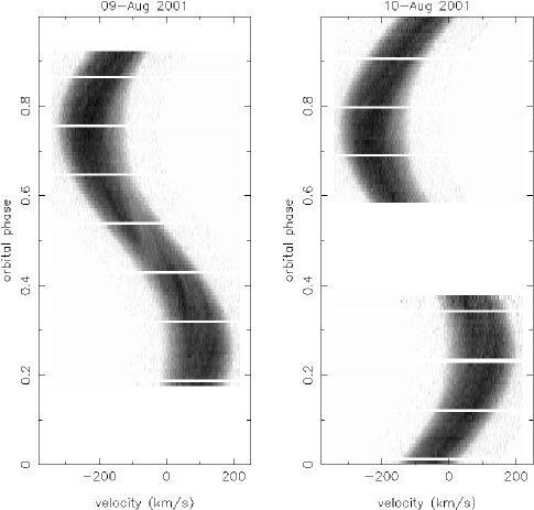
Figure 4: A trail of the deconvolved profiles from observations on 2001 August 9 (left) and 2001 August 10 (right). The small gaps in the phase coverage are at times when arc spectra were taken for the purpose of wavelength calibration. For clarity, gaps between individual exposures due to readout time are not shown. In these trailed spectra, features due to starspots will appear bright and several such features can be seen which appear on both nights (see Fig. 5 for plots with increased contrast). Also evident is the variation in $v\sin i$ showing the maximum at quadrature (phase 0.25 and 0.75) due to the changing aspect of the tidally distorted star.

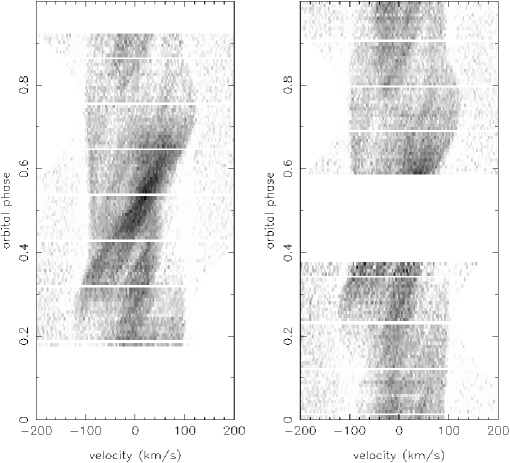
Figure 5: A trail of the deconvolved profiles from observations on 2001 August 9 (left) and 2001 August 10 (right). The orbital motion has been removed assuming the binary parameters found in Section 6, which allows the individual starspot tracks across the profiles and the variation in $v\sin i$ to be more clearly observed. In order to increase the contrast and allow the starspot features in the trailed spectrum to be more readily seen, a theoretical profile (see text) has also been subtracted from each LSD profile before trailing. In this case, starspot features now appear dark in the plots. Once again, the small gaps in the phase coverage are at times when arc spectra for the purpose of wavelength calibration were taken and gaps between individual exposures due to readout time are not shown.

4 Roche tomography

Roche tomography (Rutten & Dhillon 1994; Dhillon & Watson 2001; Watson & Dhillon 2001; Watson et al. 2003) is analogous to the Doppler imaging technique used to map rapidly rotating single stars (e.g. Vogt & Penrod 1983). Specifically, Roche tomography is designed to map the Roche-lobe-filling donor stars in interacting binaries such as CVs and X-ray binaries. In Roche tomography, the secondary star is assumed to be Roche-lobe-filling, locked in synchronous rotation and to have a circularized orbit. The secondary star is then modelled as a series of quadrilateral tiles or surface elements, each of which is assigned a copy of the local (intrinsic) specific intensity profile. These profiles are then scaled to take into account the projected area of the surface element, limb darkening and obscuration, and then Doppler shifted according to the radial velocity of the surface element at that particular phase. Summing up the contributions from each element gives the rotationally broadened profile at that particular orbital phase.

By iteratively varying the strengths of the profile contributed from each element, the ‘inverse’ of the above procedure can be performed. The spectroscopic data is fit to a target $\chi^{2}$, and a unique map is selected by employing the maximum-entropy memsys algorithm developed by Skilling & Bryan (1984). Unless otherwise stated in the text, we employ a moving uniform default map, where each element in the default is set to the average value in the reconstructed map. Since the maximum-entropy algorithm we have adopted requires that the input data is positive, we have inverted the absorption-line profiles and set any negative points to zero. For further details of the Roche tomography process see the review by Dhillon & Watson (2001).

Several Doppler imaging studies have used a two-temperature or filling-factor model (e.g. Collier Cameron & Unruh 1994) during the image reconstruction process. These studies work on the assumption that there will only be two-temperature components across the surface of the star, those of the immaculate photosphere and those of the cooler spots. Each image pixel is then effectively made up of a combination of photosphere and spot intensity. The benefits of using a two-spot model are that it ‘thresholds’ the maps, preventing the growth of bright pixels (e.g. Hatzes & Vogt 1992), and preserves the total spot areas (Collier Cameron 1992) making quantitative analysis of the maps more easy.

With Roche tomography we may well expect the secondary star to display a much more complex topography than isolated stars. In particular, the surface temperature across a CV secondary will vary greatly not just due to starspots but also as a result of irradiation, which is prominent in these systems even in single-line studies (e.g. Davey & Smith 1992; Davey & Smith 1996; Watson et al. 2003). For this reason, we cannot restrict our Roche tomograms to a two-temperature reconstruction. Thus Roche tomograms present images of the distribution of line flux on the secondary star – effectively showing the contrast between the various features, blurred by the action of the regularisation constraint.

5 Ephemeris

A new ephemeris for AE Aqr was determined by cross-correlation with a template star of spectral type K4V. We only considered the spectral region containing the strong Mg ii triplet absorption for simplicity. The AE Aqr and K4V template spectra were first normalised by dividing by a constant, and the continuum was then subtracted off using a third order polynomial fit. This procedure ensures that the line strength is preserved along the spectral region of interest.

The template spectrum was then artificially broadened to account for the rotational velocity ($v\sin i$) of the secondary star. The projected rotational broadening of the secondary star was measured using an optimal-subtraction technique in which the template spectrum was broadened, multiplied by a constant and then subtracted from an orbitally-corrected AE Aqr spectrum. The process was repeated in an iterative process, adjusting the broadening at each step, until the scatter in the residual spectrum was minimised.

Through the above process a cross-correlation function (CCF) was calculated for each AE Aqr spectrum over the wavelength region covering the strong Mg ii triplet absorption. The radial velocity curve in Fig. 6 was then obtained by fitting a sinusoid through the CCF peaks to obtain a new zero-point for the ephemeris of

$$T_{0}=\,$HJD$\,2452131.31345\pm 0.00007$$ (1)

with the orbital period fixed at $P=0.41165553$ d (from Casares et al. 1996). All subsequent analysis has been phased with respect to this new zero-point. This method of deriving the ephemeris is relatively insensitive to the use of an ill-matching template, or incorrect amount of broadening. Indeed, it is more likely to be dominated by the effects of irradiation, which is well known to introduce systematic errors in radial velocity studies if not properly accounted for (e.g. Davey & Smith 1992; Davey & Smith 1996). Although the steeper slope of the radial velocity curve around phase 0.5 suggests the presence of irradiation which is confirmed in our Roche tomograms (albeit at a low level – see section 7), the ephemeris derived here provides a substantially improved image quality (both in terms of final reduced $\chi^{2}$ and artefacts in the reconstructed map) when compared against that achieved when using the zero-point of the ephemeris published by Casares et al. (1996).

We should note that the work in this section was carried out for the sole purpose of determining a revised ephemeris in order to improve the quality of the Roche tomograms in section 7. From this perspective, no detailed attempt was made to determine the best-fitting spectral type and accurately measure the rotational broadening and other parameters from this analysis – a more traditional study along these lines will be presented in a future paper. For completeness, however, we obtained a secondary star radial velocity amplitude of $K_{r}$ = 168.4 $\pm$ 0.2 km s^-1 and a systemic velocity of $\gamma$ = –59.0 $\pm$ 1.0 km s^-1 (assuming the K4V template star HD24916A has a systemic velocity of +6.2$\pm$1.0 km s^-1, King et al. 2003). As discussed later in section 6 these measurements will be biased due to, for example, surface inhomogeneities across the secondary star and the incorrect treatment of the absorption-line profile shape (which assumes that the star is spherical). Thus, the parameters derived from the radial velocity curve have not been used in the subsequent analysis presented in this paper.

Figure 6: The measured secondary star radial-velocity curve with the best-fitting sinusoidal fit for 2001 August 9 and 10. The data have been phase folded and then repeated.

6 system parameters

As discussed in Watson & Dhillon (2001), adopting incorrect system parameters such as systemic velocity, component masses and orbital inclination when carrying out a Roche tomography reconstruction results in spurious artefacts in the final map. These artefacts normally manifest themselves in the form of bright and dark streaks and cause a decreased (more negative) entropy to result in the final map. In other-words, adopting incorrect parameters causes more structure to be mapped onto the secondary star. By carrying out reconstructions for many pairs of component masses (iterating to the same $\chi^{2}$ on each occasion) we can construct an ‘entropy landscape’ (see Fig. 9), where each grid element corresponds to the entropy value obtained in the reconstruction for a particular pair of component masses. One then adopts the set of parameters that gives the map containing the least structure (the map of maximum entropy).

For the reconstructions carried out here we have assumed a root-square limb-darkening law of the form

$$I\left(\mu\right)=I\left(1\right)\left[1-a\left(1-\mu\right)-b\left(1-\sqrt{\mu}\right)\right]$$ (2)

where $\mu=\cos\gamma$ ($\gamma$ is the angle between the line of sight and the emergent flux), and $I(1)$ is the monochromatic specific intensity at the center of the stellar disc. The limb-darkening coefficients $a=0.647$ and $b=0.213$ were adopted, which is suitable for a star of $T_{eff}$ = 4800K, $\log g$ = 4.5 at the central wavelength of our observations (Claret 1998). This form of the limb-darkening law has been chosen over the more usual linear dependency since it has been found that model atmospheres of cool stars show limb-darkening laws which are largely non-linear (e.g. Claret 1998).

To determine the binary parameters of AE Aqr, we have constructed a sequence of entropy landscapes like that described above for a range of orbital inclinations $i$ and systemic velocities $\gamma$. Then, for each $i$ and $\gamma$, we picked the maximum entropy value in the corresponding entropy landscape. From Fig. 7 this method yields a systemic velocity of $\gamma$ = –63 $\pm$ 1 km s^-1, where we have adopted the 1 km s^-1 error bar from the resolution of our grid search as a guide rather than a rigorous error estimate. This is consistent with the systemic velocity of Casares et al. (1996) who found $\gamma=-60.9\pm 2.4$ km s^-1, and is in excellent agreement with the value of –63 $\pm$ 3 km s^-1 found by Welsh, Horne & Gomer (1995). The value obtained using Roche tomography is slightly more discrepant with the value of $\gamma=-59\pm 1$ km s^-1 obtained in section 5 from the radial velocity curve. We note that the value of the systemic velocity obtained from the entropy landscape technique is constant over a wide range of assumed orbital inclinations, as found in Watson et al. (2003).

Figure 7: Points show the maximum entropy value obtained in each entropy landscape as a function of systemic velocity, assuming an orbital inclination of 66^∘. (The optimal value for the systemic velocity is, however, found to be independent of the assumed inclination). The solid curve shows a fourth order polynomial fit through these points with the intention to show more clearly where the peak in entropy occurs with respect to the assumed systemic velocity in the reconstructions.

Figure 8: Points show the maximum entropy value obtained in each entropy landscape for different inclinations, assuming a systemic velocity of $\gamma$ = –63 km s^-1. The solid curve shows a third order polynomial fit through these points. The entropy value peaks at an orbital inclination of $i=66^{\circ}$.

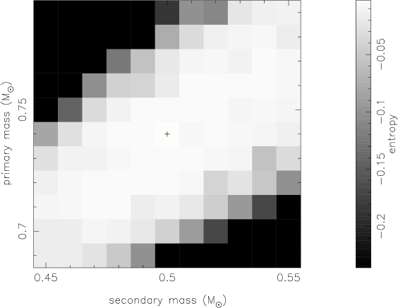
Figure 9: The entropy landscape for AE Aqr, assuming an orbital inclination of $i=66^{\circ}$ and a systemic velocity of $\gamma=-63$ km s^-1. Both nights data were combined when carrying out the reconstructions. Dark regions indicate masses for which no acceptable solution could be found. The cross marks the point of maximum entropy, corresponding to component masses of $M_{1}$ = 0.74 M_⊙ and $M_{2}$ = 0.50 M_⊙.

Fig. 8 shows the maximum-entropy value as a function of inclination obtained in entropy landscapes assuming the systemic velocity of $\gamma=-63$ km s^-1 derived above. This indicates a distinct increase in the amount of structure present in the maps either side of the best fitting inclination at $i=66^{\circ}$, which we have adopted as the optimal value for the orbital inclination of AE Aqr. It is comforting to see that this lies below the $i<70^{\circ}$ limit inferred from the lack of eclipses (Chanan, Middleditch & Nelson 1976), though it is still relatively high compared to previous estimates. Casares et al. (1996) determined $i=58^{\circ}\pm 6^{\circ}$ by modelling the phase dependent variation of the rotational broadening in their intermediate resolution spectra, while Welsh et al. (1995) constrained $i$ to $55^{\circ}\pm 7^{\circ}$ in their absorption line study of AE Aqr.

Shahbaz (1998) noted, however, that the methods used by Welsh et al. (1995) and Casares et al. (1996) to measure the orbital inclination of AE Aqr are prone to systematic errors and result in a shift to lower values for the inclination. This systematic error results from the incorrect treatment of the absorption-line profile shape which is often approximated by using the Gray profile (Gray, 1992) for spherical stars. Since the determination of the radial velocity amplitude and rotational broadening of the secondary star is also sensitive to the correct treatment of the line-profile – use of the Gray profile or failure to account for surface inhomogeneities on the secondary star can lead to systematic errors in the derived mass ratio as well. Roche tomography, however, predicts the correct broadening function for a Roche-lobe filling star and, in addition, takes into full account the line flux distribution across the star which can lead to systematic errors in these more conventional studies. Further support for the higher inclination found in this work comes from a recent preliminary analysis of high spectral-resolution data by Echevarr’ıa et al. (2005). These authors have also found evidence for a high ($\sim$70^∘) inclination from studying the phase-dependent variation of the rotational broadening.

The entropy landscape for AE Aqr assuming an orbital inclination of $i$ = 66^∘ and a systemic velocity of $\gamma$ = –63 km s^-1 is shown in Fig. 9. From this we derive a secondary star mass of $M_{2}$ = 0.50 M_⊙ and a primary mass of $M_{1}$ = 0.74 M_⊙. These are in good agreement with the most recent previous estimates in the literature, including $M_{1}$ = 0.79 $\pm$ 0.16 M_⊙ and $M_{2}$ = 0.50 $\pm$ 0.10 M_⊙ (Casares et al. 1996), as well as $M_{1}$ = 0.89 $\pm$ 0.23 M_⊙ and $M_{2}$ = 0.57 $\pm$ 0.15 M_⊙ (Welsh et al. 1995).

In all cases we have carried out reconstructions to $\chi^{2}$ = 0.8, though we have explored the effects of carrying out the reconstructions to different $\chi^{2}$ values. For reconstructions to lower $\chi^{2}$ values the entropy landscapes break up into noise, whereas when iterating to higher $\chi^{2}$ values the entropy landscapes favour higher inclinations (which are unphysical given the lack of eclipses) – eventually losing all sensitivity to the assumed inclination. In all cases, however, the derived component masses for any given orbital inclination all agree to better than 0.02M_⊙ for all reasonable selections of target $\chi^{2}$. We are confident that we are neither over-fitting nor under-fitting the data. The maps rapidly break into noise for $\chi^{2}$ values less than 0.8, leading to noisy entropy landscapes. Maps fit to greater $\chi^{2}$ values become ‘washed out’ with features becoming less distinct as more pixels are assigned the default value in the absence of proper data constraints.

It should also be noted that we have not assigned errors to our system parameter estimates. Technically, this could be done using a Monte-Carlo style technique and applying the bootstrap resampling method (Efron 1979; Efron & Tibshirani 1993) to generate synthetic datasets drawn from the same parent population as the observed dataset (see also Watson & Dhillon 2001). Unfortunately, this would mean repeating the analysis carried out in this paper for several hundred bootstrapped datasets which would require several months of computational time. It is, therefore, unfeasible for us to assign strict errors bars to our derived binary parameters. Given the quality of the data (high time and spectral-resolution) and the full treatment of the data by Roche tomography (which takes into account the roche-lobe shape and any surface inhomogeneities), we believe that the system parameters derived in this paper for AE Aqr are the most accurate to date.

7 surface maps

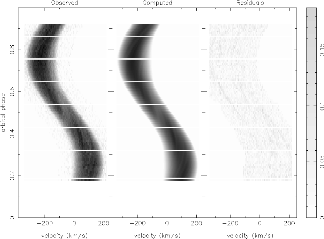
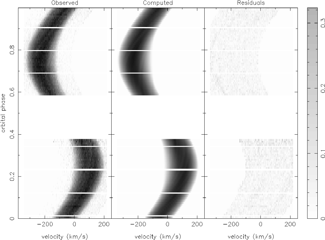
Figure 11: Roche tomography fits to the LSD trailed spectra showing the observed trails, computed trails from the Roche tomography reconstruction and the O–C residuals. The greyscale wedge (right) indicates the magnitude of the residuals as a fraction of the average line profile depth. The largest residuals result from spikes in the deconvolved continuum (which do not adversely affect the Roche tomography fits to the profiles themselves - see Figs 2 & 3). The residuals are greatest for the second nights observations due to the deterioration in the seeing at the end of the night. Top: observations from 2001 August 9. Bottom: observations from 2001 August 10.

Using the binary parameters derived in Section 6 and combining both nights datasets, we have constructed a Roche tomogram of the secondary in AE Aqr, and this is displayed in Fig. 10. The corresponding fit to the datasets obtained on both nights are displayed in Fig. 11. Dark spots are evident in the Roche tomogram. The most noticeable feature is the large starspot feature which lies near (but not centred on) the polar regions at a latitude of $\sim$65^∘ and is skewed towards the trailing hemisphere ($\phi$=0.25) of the star. Such high-latitude and polar spots are common in Doppler images of other rapidly-rotating stars and are discussed in more detail in Section 8.

The other prominent dark region in the tomogram is best seen at $\phi$=0.5. This lies at the $L_{1}$ point on the secondary star, and could possibly be due to irradiation from the accretion regions which would also appear dark in the tomograms since the weak metal lines become ionised. Although irradiation of the donor star in AE Aqr has not been seen previously, it’s location at the $L_{1}$ point is consistent with that seen in other CVs (e.g. Watson et al. 2003). Furthermore, in high spectral-resolution observations taken at the Magellan 6.5-m telescope during July 2004 (to be presented in a later paper), the preliminary LSD profiles around $\phi$=0.5 are almost identical to those presented here. This is indicative of a fixed feature around the $L_{1}$ point which is more likely due to the presence of irradiation rather than the existence of a long-lived (several year) spot feature. On the other-hand, we currently do not have a knowledge of the spot life-times for this class of star and the modelling of the mass transfer history of AM Her by Hessman et al. (2000) suggests that the spottedness of the $L_{1}$ point on the donor stars in CVs may be untypical compared to isolated stars. Despite these caveats, however, irradiation is still our preferred interpretation of the feature located at the $L_{1}$ point.

In addition to these prominent features, a number of other smaller spots can be seen at lower latitudes. Unfortunately many of these lower latitude spots are heavily smeared across the equator since the latitudinal resolution of the imaging technique decreases towards the equator (this is because the path of a starspot trail in the time series shows the least variation as a function of latitude near the equatorial regions). This problem is further compounded by the lower signal-to-noise of our LSD profiles relative to many other Doppler imaging studies of isolated stars (a result of the faintness of AE Aqr), and the target’s relatively high orbital inclination, which results in a degeneracy between which hemisphere a feature is located on (e.g. Watson & Dhillon 2001). Therefore, it is difficult to tell whether the lower latitude spots are located within a particular latitude band or not.

To check whether or not the features seen in the Roche tomogram are real, or spurious artefacts due to noise, we have carried out two further Roche tomography constructions using only the odd-numbered spectra for one and the even-numbered spectra for the other (see Fig. 13). Despite the reduction in phase-sampling, both of these Roche tomograms show the same features as seen in Fig. 10 and therefore we are confident that these features are real. Furthermore, when we construct separate maps for each nights data (not shown here for reasons outlined below), we again find that that features are reconstructed at similar locations in the maps where there is sufficient phase overlap in the observations. This gives us further confidence in the reality of the reconstructed features.

Although the maps reconstructed on individual nights show similar features, these features do differ in detail. Unfortunately, this is most likely a result of the relatively poor signal-to-noise of our observations combined with the introduction of phase gaps when reconstructing each dataset separately – further compounded by the deteriorating seeing conditions on night 2. We feel, therefore, that it would be unwise to speculate as to whether any of the detailed differences between the individual nights reconstructions are due to the evolution of spots other than to mention that there does not appear to be any significant movement of spot features. Future higher signal-to-noise observations will be better placed to resolve spot evolution.

In order to make a more quantitative estimate of the spot parameters on AE Aqr, we have examined the intensity distribution of the pixels in the Roche tomogram. By looking for a bimodal distribution in pixel intensities, an estimate of the spot properties can be obtained by labelling low-intensity pixels as spotted regions, and high-intensity pixels as immaculate photosphere. First, we discarded all pixels on the southern hemisphere as this hemisphere is least visible and as such will mainly contain pixels assigned with the default intensity which, in this case, will be the average intensity of the map. Inclusion of these pixels would ‘wash-out’ any underlying bimodal distribution in pixel intensity. The corresponding histogram of pixel values is shown in Fig. 12 and, as expected, this shows a group of pixels of lower intensity which have been labelled as starspots (see caption of Fig. 12 for details).

Although far from an ideal means of classifying what regions are spotted and what regions contain immaculate photosphere, this is the best classification scheme given our inability to apply a two-temperature model as discussed in Section 4. Based on this scheme, Fig. 14 shows the distribution of starspots as a function of latitude scaled by either the total surface area of the star, or by the surface area of the latitude strip over which the spot coverage was calculated. This confirms our visual inspection of the tomogram and that the density of spots increases towards the pole, with a grouping of spots centred around a latitude of +$65^{\circ}$ corresponding to the large spot seen near the north pole.

Inspection of Fig. 14 also shows an apparent depletion of starspots near +$40^{\circ}$, with an increase in starspot coverage again towards lower latitudes, with a further increase in spot coverage below +$10^{\circ}$. This latter increase in spots below a latitude of $\sim 10^{\circ}$ is probably due in part to the presence of irradiation near the $L_{1}$ point. Nonetheless, the irradiated region is not large enough to fully explain the increase in low-latitude pixels being flagged as spots. Therefore, this indicates the presence of a lower latitude site of magnetic activity on AE Aqr which future higher signal-to-noise observations will help resolve.

In total, we estimate that 18 per cent of the northern hemisphere on AE Aqr is spotted. We stress that this number should be regarded with caution given our scheme for classifying pixels containing spots, but that such a figure for the spot filling-factor is not at all unreasonable and, if anything, is likely to be an under-estimate of the true spot filling factor. TiO studies of rapidly rotating stars by O’Neal et al. (1998) have revealed spot filling factors as large as 50 per cent in the case of II Peg. Generally, such studies result in much larger filling factors than are deduced from Doppler images which typically return spot-filling factors from $\sim$4 per cent (e.g. Speedy Mic, 4.5 per cent, Barnes et al. 2001a) to $\sim$12 per cent (e.g. He 699, 11.9 per cent, Barnes et al. 2001b).

A prime example of the underestimation of the global spot coverage by Doppler imaging methods was highlighted by Barnes et al. (2004), whose Doppler images of the primary star in the contact binary AE Phe returned a spot filling factor of $\sim$5 per cent. Barnes et al. (2004), however, estimated that the actual spot coverage could be 27 per cent in order to lower the apparent temperature of the primary component to the level seen in their observations. This discrepancy between Doppler imaging and, for example, TiO studies is probably caused by the failure of Doppler imaging to resolve small starspots, which will certainly be the case for the lower signal-to-noise dataset presented in this paper. The poorer latitudinal resolution near the equator will also cause low-latitude spots to be heavily smeared over a larger surface area, reducing their contrast with the immaculate photosphere and increasing the probability of the non-detection of starspots at these lower latitudes. Finally, Webb et al. (2002) found a spot filling factor of 22 per cent from a TiO study of the CV SS Cyg, similar to our estimate for AE Aqr.

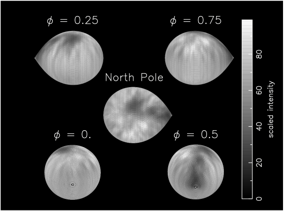
Figure 10: Roche tomogram of AE Aqr. Dark greyscales depict regions of suppressed absorption and are indicative of starspots or irradiated zones. The system is plotted as the observer would see it at an orbital inclination of 66^∘, except for the central panel which shows the system as viewed from above the North pole. The orbital phase (with respect to the ephemeris of Section 5) is indicated above each panel. For clarity, the Roche tomograms are shown excluding limb-darkening.

Figure 12: Histogram of the pixel intensities from the Roche tomogram of AE Aqr after pixels on the southern hemisphere (latitude $<$ 0^∘) were discarded. The brightest pixel in the map is assigned an intensity of 100 and other pixel intensities are scaled linearly against this. For the purposes of estimating the global spot properties of AE Aqr, the immaculate photosphere has been defined as pixels with intensities of 74 or greater, and the spotted photosphere those regions where pixel intensities are less than 74.

Figure 13: As for Fig. 10, but reconstructions for odd-numbered spectra (left) and even-numbered spectra (right).

Figure 14: Plots showing the spot coverage as a function of latitude. Left: spot coverage as a function of latitude expressed in terms of the surface area at that latitude. Right: spot coverage as a function of latitude normalised by the total surface area of the northern hemisphere. The curves appear noisy in comparison to similar plots elsewhere in the literature as the elements that make up our stellar grid are not aligned along constant latitude strips in order to ensure that the inner-Lagrangian point is tiled adequately. Therefore a certain degree of interpolation in latitude between adjacent tiles is required to calculate the contribution of each tile to that latitude.

8 Discussion

The secondary in the cataclysmic variable binary AE Aqr is a highly active star as evinced by the heavily spotted Roche tomogram presented in this work. This is unsurprising, given the rapid (0.41-d) rotation period of AE Aqr. In keeping with the abundant observations of high-latitude or polar spots on rapidly rotating stars (see Schrijver & Title 2001 and references therein), AE Aqr also exhibits a large spot at high-latitude. This spot is, however, not truly polar as seen in many Doppler images as it is centred at a latitude of around +$65^{\circ}$. This is still in striking contrast to our Sun, where starspots seldom appear beyond $\pm 30^{\circ}$ from the equator (e.g. Pulkkinen et al. 1999). After much debate about the reality of the polar spots revealed by Doppler imaging (see Hatzes et al. 1996, Unruh & Collier Cameron 1997, Bruls et al. 1998), the reality of these features now appear to be established within the field. Schüssler & Solanki (1992) have suggested that such high latitude spots are the cause of the strong Coriolis forces in these rapidly rotating stars which drive the magnetic flux tubes towards the polar regions. Alternatively, such spots can form at lower latitudes and then migrate polewards - such a poleward migration of mid-latitude spots has been reported for the RS CVn binary HR1099 (V711 Tauri – Vogt et al. 1999, Strassmeier & Bartus 2000). Future observations will be needed in order to establish whether the starspots on AE Aqr also undergo a poleward motion.

In addition, AE Aqr also appears to show starspots at latitudes below $\sim 35^{\circ}$. As described in Granzer et al. (2000), such bimodal spot distributions (the simultaneous appearance of spots at high and intermediate/low latitudes) have also been reported for the zero-age main-sequence (ZAMS) rapid rotator AB Dor (e.g. Unruh et al. 1995), the Pleiades-age main-sequence star LQ Hya (Rice & Strassmeier 1998, Donati 1999), the $\alpha$ Per G-dwarves He669 and He520 (Barnes et al. 1998), and the young G-dwarf EK Dra (Strassmeier & Rice 1998) amongst others.

In their paper studying the distribution of starspots on cool stars, Granzer et al. (2000) found that low-mass stars ($\sim 0.4$M_⊙) with rotation rates more than 4 times solar showed spot emergence at latitudes between $\sim 60-70^{\circ}$. It is perhaps worth noting that this is comparable with AE Aqr which, at 0.5M_⊙, shows spots emerging at $\sim 65^{\circ}$. Unfortunately, since AE Aqr has already evolved some way off the ZAMS, comparison to the results from modelling young stars by Granzer et al. (2000) may make any conclusion drawn from such a comparison somewhat uncertain.

It is also interesting to compare the images of AE Aqr to those of the late pre-main sequence or early ZAMS isolated star Speedy Mic (Barnes et al. 2001a). Excluding their ages and the effect of tidal forces, Speedy Mic (of spectral-type K3V and rotation period 0.38-d) otherwise has similar stellar parameters to AE Aqr ($P_{rot}$ = 0.41-d, K3-5V/IV). Like AE Aqr, Speedy Mic does not show any truly polar spot but does show a concentration of starspots around 60–70^∘ at a similar latitude to the large spot group observed on AE Aqr at 65^∘. Speedy Mic also exhibits a bimodal distribution of starspots, with a similar concentration of spots at lower latitudes to that observed for AE Aqr. Furthermore, Barnes et al. (2001a) also describe a relative paucity of spots at a latitude of 30–40^∘, the upper limit of which coincides with the depletion of spots around 40^∘ seen on AE Aqr. Such depletion of spots at intermediate latitudes is also observed in the K2 dwarf LQ Hya (Rice & Strassmeier 1998, Donati 1999) and the K5 dwarf BD +55^∘ 4409 (LO Peg – Lister, Collier Cameron & Bartus 1999). More observations of late-type stars are required in order to determine whether this feature is common to all K-type and later stars.

In conclusion, we have unambiguously imaged, for the first time, large starspots on the secondary star in AE Aqr, the distribution of which is similar to other rapidly rotating low-mass stars. We estimate a spot coverage of approximately 18 per cent, indicating a high-degree of magnetic activity which is no doubt due to an efficient dynamo driven by rapid rotation. Such a high-level of activity on AE Aqr provides evidence that magnetic-braking in long-period CVs could play a significant role in their evolution towards the period gap.

9 Future opportunities

Given that this is the first time that starspots have been imaged on the secondary stars in CVs, we thought it prudent to discuss the future avenues that such studies could explore.

9.1 Spot properties on CV secondaries

As briefly mentioned in Section 1, a knowledge of the distribution of starspots on Roche-lobe filling stars can provide tests of our understanding of stellar dynamos. For example, the models of Holzwarth & Schüssler (2003) show that the tidal effects in a binary due to the presence of a close companion can lead to the formation of clusters of flux tubes (and therefore starspots) at preferred longitudes. Furthermore, these effects are predicted to become more pronounced for shorter period systems where the tidal forces are strongest. Since CVs contain some of the most rapidly rotating stars known, they provide excellent candidates in which to study the effects of tidal forces on magnetic flux tube emergence. In addition, since the magnitude of the tidal effects will change with changing binary parameters, so will the predicted starspot distributions. Therefore it is highly desirable to obtain a set of high-resolution maps of a number of different CVs as each individual binary system studied should, in principle, provide an independent test of such models.

Studies should also be carried out to investigate how the starspot coverage varies with time in an attempt to deduce whether these stars display magnetic activity cycles similar to the 11-year solar cycle. An understanding of these cycles is crucial to the success of any stellar dynamo theory. As outlined in Section 1, magnetic activity cycles have also been invoked to explain quasi-cyclical variations in orbital periods, quiescent magnitudes and outburst intervals, durations and shapes, with cycles on timescales as short as $\sim$ 3 years (Ak, Ozkan & Mattei, 2001). No direct evidence for magnetic activity cycles has so far been found for these systems and therefore long-term monitoring of a selection of CVs is actively encouraged. To this end we have initiated a long-term monitoring campaign of AE Aqr, the first results of which are to be published in a future paper.

9.2 Differential rotation of tidally distorted stars

Differential rotation is thought to play a crucial role in amplifying and transforming the initial poloidal magnetic field into toroidal field through dynamo processes (the so-called $\Omega$ effect). Thus measurements of differential rotation rates aim to evaluate the influence of stellar parameters on the surface shear rates and hence test stellar dynamo theories. Theoretical work regarding differential rotation in tidally distorted stars by Scharlemann (1982) suggests that it should be weakened, but not entirely suppressed, in these objects. Some two decades later, however, observational evidence for the strength of differential rotation in tidally distorted stars is still confused. Petit et al. (2004) find evidence for weak differential rotation in the RS CVn system HR 1099. Images of the contact binary AE Phe (Barnes et al., 2004), on the other-hand, shows rapid spot evolution and motions. Evidently more studies of tidally distorted systems are required.

By acquiring two images of a CV separated by several days, one can cross-correlate strips of constant latitude, allowing the sense and magnitude of the differential rotation to be measured. Furthermore, in the event that surface shear exists, Scharlemann (1982) note that, on average, the stellar envelope should still be forced to co-rotate. Roche tomography studies could also be used to deduce the co-rotation latitude at which the envelope is tidally-locked to the orbital period.

Although fainter than RS CVn systems, CVs still offer an excellent laboratory to study differential rotation in tidally distorted stars. For instance, RS CVn’s have orbital periods that typically span several days, meaning that long observations covering several nights are required to establish a complete picture of the system. During this time individual starspots may have appeared, evolved into different shapes or disappeared entirely. Therefore a single image of an RS CVn system can often not be regarded as a single ‘snapshot’ of the spot morphology – making the detection and accurate determination of differential rotation rates more complicated. CVs, however, have shorter orbital periods (typically $<$ 10 hours) and therefore a single Roche tomogram of a CV should be obtainable in one night for the majority of cases – making differential rotation studies more accessible.

9.3 Impact of activity on accretion dynamics

Magnetic activity on the secondary stars in CVs is also thought to play a role in the accretion dynamics of interacting binaries over short timescales. Livio & Pringle (1994) have suggested that the low states observed in some interacting binaries can be explained by the passage of starspots across the inner-Lagrangian ($L_{1}$) point (see also King & Cannizzo 1998). This temporarily quenches the flow of material through the $L_{1}$ point, thereby reducing the accretion rate. Indeed, Hessman et al. (2000) were able to model the long-term brightness variations of the cataclysmic variable AM Her as modulations caused by starspots and conclude that either these systems have a large spot covering fraction ($\sim$ 0.5) or that the $L_{1}$ point is unusually spotty. More recently, de Martino et al. (2002) also attributed the rapid variation of accretion in Am Her to starspots. Such mass transfer variations can also have a marked effect on the response of the accretion disc in dwarf novae (Schreiber et al. 2000).

There are a number of ways that these ideas can be tested with Roche tomography. First, the observation of a starspot crossing the $L_{1}$ point in combination with a simultaneous drop in system brightness (high-resolution Roche tomography datasets should normally be accompanied by simultaneous photometry) would provide evidence supporting these models. Although such an observation may seem fortuitous, given the large spot coverages seen on rapidly rotating stars (as much as 50 per cent, O’Neal et al. 1996) and, in particular, given the high spot coverages seen in the Roche tomograms of AE Aqr, there is a high probability of witnessing such an event. The main problem with this approach would be assessing whether a feature at the $L_{1}$ point was truly a spot or caused by irradiation. One suitable target is the bright Z Cam type dwarf-nova V426 Oph (Hellier et al. 1990) which exhibits drops from standstill which may be due to a decrease in mass transfer. (In recent high-resolution Magellan observations starspot features were found in the deconvolved line profiles of V426 Oph and a Roche tomogram of V426 Oph will be published in a later paper).

Second, even if an event is not seen directly, given a detailed knowledge of the starspot distributions and the sense and magnitude of their motions of the starspots due to differential rotation (Section 9.2), it should be possible to predict at what times a starspot will migrate across the $L_{1}$ point. Again, an observed dimming at the predicted times would provide strong evidence in favour of such models. Furthermore, King & Cannizzo (1998) note that the most rapid transitions to low states occur over the course of a day. The length scale of the mass overflow region near the $L_{1}$ point is (e.g. Pringle 1985)

$$w\simeq\frac{Pc_{s}}{2\pi}\simeq 3\times 10^{8}P_{hr}~{}{\rm cm},$$ (3)

where $c_{s}$ is the sound speed of the gas and $P_{hr}$ is the orbital period $P$ expressed in hours. In order to cause a transition to a low-state over one day, a spot boundary would have to move across the $L_{1}$ point at a velocity of $\sim$ 3 $\times$ 10${}^{3}P_{hr}$ cm s^-1. By using starspots as surface flow tracers it will be possible to determine whether the differential rotation rates in CVs are commensurate with these velocities.

Finally, in the model for AM Her proposed by Hessman et al. (2000), they infer a power-law for the distribution of spot sizes. Using Roche tomography, one can determine both the numbers and sizes of the starspots on CV secondary stars, allowing the measurement of the power-law index for the upper end of the spot size distribution (e.g. Collier Cameron 2001). This would provide a powerful consistency test for such models.

In conclusion, not only are Roche tomography studies important for our further understanding of the diverse behaviour of CVs but they also promise to provide further insights into stellar dynamos. In order to provide the best constraints on spot sizes and distributions, and to extend surveys to more (and almost certainly fainter) CVs, observations using echelle spectrographs on 6 to 8-m class telescopes will be required.

References

- Ak et al. (2001) Ak T., Ozkan M. T., Mattei J. A., 2001, A&A, 369, 882
- Andronov et al. (2003) Andronov N., Pinsonneault M., Sills A., 2003, ApJ, 582, 358
- Applegate (1992) Applegate J. H., 1992, ApJ, 385, 621
- Barnes (1999) Barnes J. R., 1999, PhD thesis, University of St. Andrews
- Barnes & Collier Cameron (2001) Barnes J. R., Collier Cameron A., 2001, MNRAS, 326, 950
- Barnes et al. (2000) Barnes J. R., Collier Cameron A., James D., Donati J.-F., 2000, MNRAS, 314, 162
- Barnes et al. (001a) Barnes J. R., Collier Cameron A., James D., Donati J.-F., 2001a, MNRAS, 324, 231
- Barnes et al. (001b) Barnes J. R., Collier Cameron A., James D. J., Steeghs D., 2001b, MNRAS, 326, 1057
- Barnes et al. (1998) Barnes J. R., Collier Cameron A., Unruh Y. C., Donati J. F., Hussain G. A. J., 1998, MNRAS, 299, 904
- Barnes et al. (2004) Barnes J. R., Lister T., Hilditch R., Collier Cameron A., 2004, MNRAS, 348, 1321
- Beskrovnaya et al. (1996) Beskrovnaya N. G., Ikhsanov N. R., Bruch A., Shakhovskoy N. M., 1996, A&A, 307, 840
- Bruch (1991) Bruch A., 1991, A&A, 251, 59
- Bruls et al. (1998) Bruls J. H. M. J., Solanki S. K., Schüssler M., 1998, A&A, 336, 231
- Casares et al. (1996) Casares J., Mouchet M., Martinez-Pais I. G., Harlaftis E. T., 1996, MNRAS, 282, 182
- Chanan et al. (1976) Chanan G. A., Middleditch J., Nelson J. E., 1976, ApJ, 208, 512
- Claret (1998) Claret A., 1998, A&A, 335, 647
- Collier Cameron (1992) Collier Cameron A., 1992, in Byrne P. B., Mullan D. J., eds, Surface Inhomogeneities on Late-type Stars Springer Verlag, p. 33
- Collier Cameron (2001) Collier Cameron A., 2001, in Boffin H., Steeghs D., eds, Astrotomography: Indirect Imaging Methods in Observational Astronomy Springer-Verlag Lecture Notes in Physics, Berlin, p. 183
- Collier Cameron & Unruh (1994) Collier Cameron A., Unruh Y. C., 1994, MNRAS, 269, 814
- Crawford & Kraft (1956) Crawford J. A., Kraft R. P., 1956, ApJ, 123, 44
- Davey & Smith (1992) Davey S., Smith R. C., 1992, MNRAS, 257, 476
- Davey & Smith (1996) Davey S., Smith R. C., 1996, MNRAS, 280, 481
- de Martino et al. (2002) de Martino D., Matt G., Gänsicke B. T., Silvotti R., Bonnet-Bidaud J. M., Mouchet M., 2002, A&A, 396, 213
- Dhillon & Watson (2001) Dhillon V. S., Watson C. A., 2001, in Boffin H., Steeghs D., eds, Astrotomography: Indirect Imaging Methods in Observational Astronomy Springer-Verlag Lecture Notes in Physics, Berlin, p. 94
- Donati (1999) Donati J.-F., 1999, MNRAS, 302, 457
- Donati et al. (1997) Donati J.-F., Semel M., Carter B. D., Rees D. E., Collier Cameron A., 1997, MNRAS, 291, 658
- Echevarr\a’ıa et al. (2005) Echevarr\a’ıa J., Smith R. C., Pineda L., Costero R., Zharikov S., Michel R., Spruit H., 2005, MNRAS, to be submitted
- Efron (1979) Efron B., 1979, Annals of Statistics, 7, 1
- Efron & Tibshirani (1993) Efron B., Tibshirani R. J., 1993, An Introduction to the Bootstrap. Chapman & Hall, New York
- Eracleous & Horne (1996) Eracleous M., Horne K. D., 1996, ApJ, 471, 427
- Granzer et al. (2000) Granzer T., Schüssler M., Caligari P., Strassmeier K. G., 2000, A&A, 355, 1087
- Gray (1992) Gray D. F., 1992, The Observations and Analysis of Stellar Photospheres. Wiley-Interscience, New York
- Hatzes & Vogt (1992) Hatzes A. P., Vogt S. S., 1992, MNRAS, 258, 387
- Hatzes et al. (1996) Hatzes A. P., Vogt S. S., Ramseyer T. F., Misch A., 1996, AJ, 469, 808
- Hellier et al. (1990) Hellier C., O’Donoghue D., Buckley D., Norton A., 1990, MNRAS, 242, 32
- Henden & Honeycutt (1995) Henden A. A., Honeycutt R. K., 1995, PASP, 107, 324
- Hessman et al. (2000) Hessman F. V., Gänsicke B. T., Mattei J. A., 2000, A&A, 361, 952
- Holzwarth & Schüssler (2003) Holzwarth V., Schüssler M., 2003, A&A, 405, 303
- Horne (1986) Horne K., 1986, pasp, 98, 609
- Jeffers et al. (2002) Jeffers S. V., Barnes J. R., Collier Cameron A., 2002, MNRAS, 331, 666
- King & Cannizzo (1998) King A. R., Cannizzo J. K., 1998, ApJ, 499, 348
- King et al. (2003) King J. R., Villarreal A. R., Soderblom D. R., Gulliver A. F., Adelman S. J., 2003, AJ, 125, 1980
- Kraft (1967) Kraft R. P., 1967, ApJ, 150, 551
- Kupka et al. (1999) Kupka F., Piskunov N. E., Ryabchikova T. A., Stempels H. C., W. W. W., 1999, A&AS, 138, 119
- Kupka et al. (2000) Kupka F. G., Ryabchikova T. A., Piskunov N. E., Stempels H. C., W. W. W., 2000, Baltic Astronomy, 9, 590
- Lister et al. (1999) Lister T., Collier Cameron A., Bartus J., 1999, MNRAS, 307, 685
- Livio & Pringle (1994) Livio M., Pringle J. E., 1994, ApJ, 427, 956
- Marsden et al. (2005) Marsden S. C., Waite I. A., Carter B. D., Donati J. F., 2005, MNRAS, 359, 711
- Mauche et al. (1997) Mauche C. W., Lee P. Y., Kallman T. R., 1997, ApJ, 477, 832
- Mestel (1968) Mestel L., 1968, MNRAS, 138, 359
- O’Neal et al. (1996) O’Neal D., Saar S. H., Neff J. E., 1996, ApJ, 463, 766
- O’Neal et al. (1998) O’Neal D., Saar S. H., Neff J. E., 1998, ApJ, 501, L73
- Pearson et al. (2003) Pearson K. K., Horne K., Skidmore W., 2003, MNRAS, 338, 1067
- Petit et al. (2004) Petit P., Donati J.-F., Wade G. A., Landstreet J. D., Bagnulo S., Lüftinger T., Sigut T. A. A., Shorlin S. L. S., Strasser S., Aurière M., Oliveira J. M., 2004, MNRAS, 348, 1175
- Pringle (1985) Pringle J. E., 1985, in Pringle J. E., Wade R. A., eds, , Interacting Binary Stars. Cambridge University Press, Cambridge, p. 1
- Pulkkinen et al. (1999) Pulkkinen P. J., Brooke J., Pelt J., Tuominen I., 1999, A&A, 341, L43
- Reinsch & Beuermann (1994) Reinsch K., Beuermann K., 1994, A&A, 282, 493
- Rice & Strassmeier (1998) Rice J. B., Strassmeier K. G., 1998, A&A, 336, 972
- Richman et al. (1994) Richman H. R., Applegate J. H., Patterson J., 1994, PASP, 106, 1075
- Rutten (1987) Rutten R. G. M., 1987, A&A, 177, 131
- Rutten & Dhillon (1994) Rutten R. G. M., Dhillon V. S., 1994, A&A, 288, 773
- Scharlemann (1982) Scharlemann E. T., 1982, ApJ, 253, 298
- Schenker et al. (2002) Schenker K., King A. R., Kolb U., Wynn G. A., Zhang Z., 2002, MNRAS, 337, 1105
- Schreiber et al. (2000) Schreiber M. R., Gänsicke B. T., Hessman F. V., 2000, A&A, 358, 221
- Schrijver & Title (2001) Schrijver C. J., Title A. M., 2001, AJ, 551, 1099
- Schüssler & Solanki (1992) Schüssler M., Solanki S. K., 1992, A&A, 355, 1087
- Shahbaz (1998) Shahbaz T., 1998, MNRAS, 298, 153
- Skidmore et al. (2003) Skidmore W., O’Brien K., Horne K., Gomer R., Oke J. B., Pearson K. J., 2003, MNRAS, 338, 1057
- Skilling & Bryan (1984) Skilling J., Bryan R. K., 1984, MNRAS, 211, 111
- Spruit & Ritter (1983) Spruit H. C., Ritter H., 1983, A&A, 124, 267
- Strassmeier & Bartus (2000) Strassmeier K. G., Bartus J., 2000, A&A, 354, 537
- Strassmeier & Rice (1998) Strassmeier K. G., Rice J. B., 1998, A&A, 330, 685
- Taam & Spruit (1989) Taam R. E., Spruit H. C., 1989, ApJ, 345, 972
- Tanzi et al. (1981) Tanzi E. G., Chincarini G., Tarenghi M., 1981, PASP, 93, 68
- Unruh & Collier Cameron (1997) Unruh Y. C., Collier Cameron A., 1997, MNRAS, 290, L37
- Unruh et al. (1995) Unruh Y. C., Collier Cameron A., Cutispoto G., 1995, MNRAS, 277, 1145
- Vogt et al. (1999) Vogt S. S., Hatzes A. P., Misch A. A., Kürster M., 1999, ApJS, 121, 547
- Vogt & Penrod (1983) Vogt S. S., Penrod G. D., 1983, PASP, 95, 565
- Wade et al. (2000) Wade G. A., Donati J.-F., Landstreet J. D., Shorlin S. L. S., 2000, MNRAS, 313, 823
- Wade (1982) Wade R. A., 1982, AJ, 87, 1558
- Watson & Dhillon (2001) Watson C. A., Dhillon V. S., 2001, MNRAS, 326, 67
- Watson et al. (2003) Watson C. A., Dhillon V. S., Rutten R. G. M., Schwope A. D., 2003, MNRAS, 341, 129
- Webb et al. (2002) Webb N. A., Naylor T., Jeffries R. D., 2002, ApJ, 568, 45
- Welsh et al. (1995) Welsh W. F., Horne K., Gomer R., 1995, MNRAS, 275, 649
- Welsh et al. (1993) Welsh W. F., Horne K., Oke J. B., 1993, ApJ, 406, 229
- Wynn et al. (1997) Wynn G. A., King A. R., Horne K., 1997, MNRAS, 286, 436