The large scale clustering of radio sources

Abstract

The observed two-point angular correlation function, $w(\theta)$, of mJy radio sources exhibits the puzzling feature of a power-law behaviour up to very large ($\sim 10^{\circ}$) angular scales which cannot be accounted for in the standard hierarchical clustering scenario for any realistic redshift distribution of such sources. After having discarded the possibility that the signal can be explained by a high density local ($z\mathrel{\hbox to0.0pt{\lower 3.0pt\hbox{$\sim$}\hss}\raise 2.0pt\hbox{$<$}}0.1$) source population, we find no alternatives to assuming that – at variance with all the other extragalactic populations studied so far, and in particular with optically selected quasars – radio sources responsible for the large-scale clustering signal were increasingly less clustered with increasing look-back time, up to at least $z\simeq 1$. The data are accurately accounted for in terms of a bias function which decreases with increasing redshift, mirroring the evolution with cosmic time of the characteristic halo mass, $M_{\star}$, entering the non linear regime. In the framework of the ‘concordance cosmology’, the effective halo mass controlling the bias parameter is found to decrease from about $10^{15}\,M_{\odot}/h$ at $z\simeq 0$ to the value appropriate for optically selected quasars, $\simeq 10^{13}\,M_{\odot}/h$, at $z\simeq 1.5$. This suggests that, in the redshift range probed by the data, the clustering evolution of radio sources is ruled by the growth of large-scale structure, and that they are associated with the densest environments virializing at any cosmic epoch. The data provide only loose constraints on radio source clustering at $z\mathrel{\hbox to0.0pt{\lower 3.0pt\hbox{$\sim$}\hss}\raise 2.0pt\hbox{$>$}}1$ so we cannot rule out the possibility that at these redshifts the clustering evolution of radio sources enters a different regime, perhaps similar to that found for optically selected quasars. The dependence of the large-scale shape of $w(\theta)$ on cosmological parameters is also discussed.

1 Introduction

Extragalactic radio sources are well suited to probe the large scale structure of the Universe since they are detected over large cosmological distances (up to $z\sim 6$), are unaffected by dust extinction, and can thus provide an unbiased sampling of volumes larger than those usually probed by optical surveys. On the other hand, their 3D-space distribution can be recovered only in the very local Universe ($z\mathrel{\hbox to0.0pt{\raise-1.29167pt\hbox{${\scriptstyle\sim}$}\hss}\raise 2.58334pt\hbox{${\scriptstyle<}$}}0.1$; see Peacock $\&$ Nicholson 1991; Magliocchetti et al. 2004) because the majority of radio galaxies detected in the available large area surveys, carried out at low frequencies, have very faint optical counterparts, so that measurements of their redshifts are a difficult task. As a result, only the angular clustering can be measured for the radio source population. Interestingly, high-frequency surveys have much higher identification rates (Ricci et al. 2004), suggesting that this difficulty may be overcome when such surveys will cover sufficiently large areas.

Even the detection of clustering in the 2D distribution of radio sources proved to be extremely difficult (see Webster 1976, Seldner $\&$ Peebles 1981, Shaver $\&$ Pierre 1989) since, when projected onto the sky, the space correlation is significantly diluted because of the broad redshift distribution of radio sources. It was only with the advent of deep radio surveys covering large areas of the sky, such as the FIRST (Becker, White $\&$ Helfand 1995), WENSS (Rengelink et al. 1997), NVSS (Condon et al. 1998), and SUMSS (Bock, Large $\&$ Sadler 1999), that the angular clustering of this class of objects has been detected with a high statistical significance down to flux density limits of few mJy (see Cress et al. 1997 and Magliocchetti et al. 1998, 1999 for the FIRST survey; Blake $\&$ Wall 2002a,b and Overzier et al. 2003 for NVSS; Rengelink $\&$ Röttgering 1999 for WENSS and Blake, Mauch $\&$ Sadler 2004 for SUMSS). Amongst all the above surveys, NVSS is characterized by the most extensive sky coverage and can thus take advantage of high statistics despite its relatively high flux limit ($\sim 3\,$mJy vs $\sim 1\,$mJy of FIRST). The two-point angular correlation function, $w(\theta)$, measured for NVSS sources brighter than 10 mJy is well described by a power-law, extending from $\sim 0.1$ degrees up to scales of almost 10 degrees. A signal of comparable amplitude and shape was detected in the FIRST survey at the same flux density limit, on scales of up to 2-3 degrees (see e.g. Magliocchetti et al. 1999), while at larger angular separations any positive clustering signal - if present - was hidden by the noise.

Most analyses of radio source clustering performed so far (see e.g. Blake $\&$ Wall 2002a,b; Overzier et al. 2003) assume a two-point spatial correlation function of the form $\xi_{\rm rg}(r)=(r/r_{0})^{-\gamma}$. The power-law shape is in fact preserved when projected onto the sky (see Limber 1953), so that the observed behaviour of the angular correlation is well recovered. The studies summarized by Overzier et al. (2003) typically found correlation lengths $r_{0}$ in the range 5–15$\,h^{-1}\,$Mpc. This large range may reflect on one hand real differences in the correlation properties of radio sources of different classes/luminosities, and, on the other hand, the large uncertainties on both the redshift distribution of the sources and the time-evolution of clustering, which are necessary ingredients to estimate $\xi_{\rm rg}(r)$ from the observed $w(\theta)$.

Overzier et al. (2003) found that the observed clustering of powerful radio sources is consistent either with an essentially redshift independent comoving correlation length $r_{0}=14\pm 3\,h^{-1}\,$Mpc, close to that measured for extremely red objects (EROs) at $z\simeq 1$ (Daddi et al. 2001) or with a galaxy conservation model, whereby the clustering evolution follows the cosmological growth of density perturbations. In the latter case, the present-day value of $r_{0}$ for the most powerful radio sources is comparable to that of local rich clusters.

A deeper examination of the power-law behaviour of the angular two-point correlation function up to scales of the order of $\sim 10^{\circ}$ highlights some interesting issues. In fact, within the Cold Dark Matter paradigm of structure formation, the spatial correlation function of matter displays a sharp cut-off around a comoving radius of $r\sim 100\,\hbox{Mpc}$ (see e.g. Matsubara 2004, Fig. 1), which, at the average redshift for radio sources $<z>\sim 1$, corresponds to angular separations of only a few ($\sim 1^{\circ}-2^{\circ}$) degrees, in clear contrast with the observations. This opens the question of how to reconcile the clustering properties of these sources with the standard scenario of structure formation. Magliocchetti et al. (1999) claim that the large-scale positive tail of the angular correlation function $w(\theta)$ can be reproduced by allowing for a suitable choice of the time-evolution of the bias parameter, characterizing the way radio galaxies trace the underlying mass distribution. Although promising, this approach suffers from a number of limitations due to both theoretical modelling and the quality of data then available.

The aim of the present work is therefore to investigate in better detail and to provide a self-consistent explanation of the puzzling behaviour of the angular correlation function of radio sources, especially on large angular scales. We will concentrate on the results from the NVSS survey (Blake & Wall 2002b; Overzier et al. 2003) as, thanks to the extremely good statistics, a clear detection of a positive clustering signal was obtained up to $\sim 10^{\circ}$. We will exploit the available spectroscopic information on local radio sources to limit the uncertainties on their redshift distribution, and will mainly focus on the time evolution of their clustering properties via the bias parameter. In this way we will derive interesting constraints on the typical mass of dark matter halos hosting the population of radio sources. We will also investigate the dependence of the predicted angular correlation function on cosmological parameters.

The layout of the paper is as follows. A short description of the NVSS survey is presented in Section 2. Section 3 illustrates the adopted model for the redshift distribution of mJy radio sources, while in Section 4 we provide the formalism for the two-point angular correlation function. Results and discussions are presented in Section 5. In Section 6 we summarize our main conclusions.

2 The NVSS survey

The NVSS (NRAO VLA Sky Survey, Condon et al. 1998) is the largest radio survey that currently exists at $1.4\,$GHz. It was constructed between 1993 and 1998 and covers $\sim 10.3\,$sr of the sky north of $\delta=-40^{\circ}$. The survey was performed with the VLA in the D configuration and the full width at half-maximum (FWHM) of the synthesized beam is 45 arcsec. The source catalogue contains 1.8$\times$10⁶ sources and it is claimed to be 99 per cent complete above the integrated flux density S${}_{\rm 1.4GHz}=3.5\,$mJy.

The two-point angular correlation function, $w(\theta)$, of NVSS sources has been measured by Blake $\&$ Wall (2002a, 2002b) and Overzier et al. (2003) for different flux-density thresholds between 3 mJy and 500 mJy. The overall shape of $w(\theta)$ is well reproduced by a double power-law. On scales below $\sim 0.1^{\circ}$, the steeper power-law reflects the distribution of the resolved components of single giant radio sources. On larger scales the shallower power-law describes the correlation between distinct radio sources. Since the behaviour on small scales is mainly determined by the joint effect of the astrophysical properties of the sources and of the resolution of VLA in the various configurations, while that on larger scales is of cosmological origin, we will concentrate on the latter only. In fact, the clustering behaviour on scales $\mathrel{\hbox to0.0pt{\lower 3.0pt\hbox{$\sim$}\hss}\raise 2.0pt\hbox{$>$}}0.1^{\circ}$ provides insights on both the nature of the radio sources, through the way in which they trace the underlying dark matter distribution, and on the cosmological framework which determines the distribution of dark matter at each epoch.

We will consider the two-point angular correlation function as measured by Blake $\&$ Wall (2002b) for sources with $S_{1.4GHz}\geq 10$ mJy. Such a flux limit ensures the survey to be complete and, at the same time, provides good enough statistics to measure angular clustering up to very large scales with small uncertainties. Moreover, this limit also represents the deepest flux-density for which systematic surface density gradients are approximately negligible (Blake & Wall 2002a). The NVSS source surface density at this threshold is 16.9 deg^-2.

The data corresponding to separations in the range $0.1^{\circ}\mathrel{\hbox to0.0pt{\lower 3.0pt\hbox{$\sim$}\hss}\raise 2.0pt\hbox{$<$}}\theta\mathrel{\hbox to0.0pt{\lower 3.0pt\hbox{$\sim$}\hss}\raise 2.0pt\hbox{$<$}}0.3^{\circ}$ most likely suffer from a deficit of pairs probably due to an imperfect cleaning of bright side lobes (see Blake, Mauch $\&$ Sadler, 2004). Therefore in the following we will only consider scales $\theta>0.3^{\circ}$. In this range of scales, the measured angular correlation function is found to be described as a power law, $w(\theta)=1.49\cdot 10^{-3}\times\theta^{-1.05}$, with $\theta$ in degrees (see Blake, Mauch $\&$ Sadler 2004).

3 Redshift distribution of milliJansky radio sources

Figure 1: Adopted redshift distribution per unit redshift interval, ${\mathcal{N}}(z)$, for the radio source population with $S_{1.4{\rm GHz}}\geq 10\,$mJy. The dashed line represents the contribution of AGN-powered radio sources according to the PLE model of DP90, while the dotted line shows the contribution from star-forming galaxies obtained by Magliocchetti et al. (2002).

In order to provide theoretical predictions for the angular two-point correlation function of a given class of objects it is necessary to know their redshift distribution, ${\mathcal{N}}(z)$, i.e. the number of objects per unit comoving volume as a function of redshift. Unfortunately, the redshift distribution of mJy radio sources is not yet accurately known as the majority of radio sources powered by Active Galactic Nuclei (AGN) – which dominate the mJy population – are located at cosmological distances ($<z>\sim 1$) and are in general hosted by galaxies which are optically extremely faint.

A large set of models for the epoch-dependent Radio Luminosity Function (hereafter RLF) are available in literature (see e.g. Dunlop $\&$ Peacock 1990, Rowan-Robinson et al. 1993, Toffolatti et al. 1998, Jackson $\&$ Wall 1999, Willot et al. 2001), but they all suffer from the fact that they are mainly based on, and constrained by data sets which include only bright sources ($S_{1.4GHz}\mathrel{\hbox to0.0pt{\raise-1.29167pt\hbox{${\scriptstyle\sim}$}\hss}\raise 2.58334pt\hbox{${\scriptstyle>}$}}100\,$mJy) so that any extrapolation of their predictions to lower fluxes is quite uncertain. Amongst all the available RLFs, those provided by Dunlop $\&$ Peacock (1990, hereafter DP90) are the most commonly used to infer the redshift distribution of radio sources at the mJy level. DP90 derived their set of RLFs on the basis of spectroscopically complete samples from several radio surveys at different frequencies. By using a ‘maximum entropy’ analysis they determined polynomial approximations to the luminosity function and its evolution with redshift which were all consistent with the data available at that time. In addition, they also proposed two models of a more physical nature, assuming either Pure Luminosity Evolution (hereafter PLE) or Luminosity/Density Evolution.

Recently, with the aim of determining the photometric and spectroscopic properties for at least the population of local (i.e. $z<0.2$) radio sources at the mJy level, a number of studies have concentrated on samples obtained combining radio catalogues like FIRST and NVSS with optical ones like SDSS and 2dFGRS (Sadler et al. 2002, Ivezi$\acute{c}$ et al. 2002, Magliocchetti et al. 2002, 2004). The radio/optical samples obtained in this way provide a crucial constraint at $z\sim 0$ for any theoretical model aiming at describing the epoch-dependent RLF.

For instance, Magliocchetti et al. (2002, hereafter M02) have shown that the RLF at 1.4 GHz derived from all the objects in their spectroscopic sample having $S\geq 1$ mJy and $b_{J}\leq 19.45$, is well reproduced at relatively high radio luminosities ($P_{1.4{\rm GHz}}>10^{20.5}\,\hbox{W}\,\hbox{Hz}^{-1}\,\hbox{sr}^{-1}$) by the DP90’s PLE model for steep-spectrum FRI-FRII sources (Fanaroff $\&$ Riley 1974). At lower radio luminosities, where the radio population is dominated by star-forming galaxies, the measured RLF is better described by the one proposed by Saunders et al. (1990) for IRAS galaxies (see also Rowan-Robinson et al. 1993), although with a small adjustment of the parameters.

Following to M02, we adopt the DP90 PLE model to derive the redshift distribution of AGN-fuelled radio sources with $S_{1.4{\rm GHz}}\geq 10\,$mJy (see Fig. 1, dashed line). We will not take into account the other DP90 models, since we have found them to be inconsistent with the local RLF. In fact, while the model assuming density/luminosity evolution over-predicts the number of steep-spectrum radio galaxies below $P_{1.4{\rm GHz}}\mathrel{\hbox to0.0pt{\raise-1.29167pt\hbox{${\scriptstyle\sim}$}\hss}\raise 2.58334pt\hbox{${\scriptstyle<}$}}10^{22}\,\hbox{W}\,\hbox{Hz}^{-1}\,\hbox{sr}^{-1}$, models using polynomial approximations for the RLF give an unrealistic overestimate of the number of local sources at every luminosity.

We will also use the fit provided by M02 to the local RLF in order to estimate the redshift distribution of star-forming radio galaxies with $S_{1.4{\rm GHz}}\geq 10\,$mJy (see Fig. 1, dotted line). Note that star-forming galaxies comprise less than 30% of the $z\mathrel{\hbox to0.0pt{\raise-1.29167pt\hbox{${\scriptstyle\sim}$}\hss}\raise 2.58334pt\hbox{${\scriptstyle<}$}}0.1$ population of radio sources with $S_{1.4{\rm GHz}}\geq 10\,$mJy, and only $\simeq 0.5\%$ of the total counts at this flux limit. As we will show in the next Section, this result implies that the contribution of star-forming galaxies to the large scale angular clustering of NVSS sources is totally negligible.

4 model for the angular correlation function

The two-point angular correlation function, $w(\theta)$, of a population of extragalactic sources is related to their spatial correlation function, $\xi(r,z)$, and to their redshift distribution via the Limber’s (1953) equation:

$$w(\theta) = \int_{{\mathcal{Z}}}dz{\mathcal{N}}^{2}(z)\int_{{\mathcal{Z}}^{\prime}(z)}d(\delta z)\xi[r(\delta z,\theta),z]$$ (1)

$$\times\left[\int_{{\mathcal{Z}}}dz{\mathcal{N}}(z)\right]^{-2}.$$

In this expression, $r(\delta z,\theta)$ is the comoving spatial distance between two objects located at redshifts $z$ and $z+\delta z$ and separated by an angle $\theta$ on the sky. For a flat universe and in the small angle approximation (which is still reasonably accurate for the scales of interest here, i.e. $0.3^{\circ}\mathrel{\hbox to0.0pt{\raise-1.29167pt\hbox{${\scriptstyle\sim}$}\hss}\raise 2.58334pt\hbox{${\scriptstyle<}$}}\theta\mathrel{\hbox to0.0pt{\raise-1.29167pt\hbox{${\scriptstyle\sim}$}\hss}\raise 2.58334pt\hbox{${\scriptstyle<}$}}10^{\circ}$),

$$r^{2}=\left(\frac{c}{H(z)}\right)^{2}\delta z^{2}+d^{2}_{\theta}(z),$$ (2)

where $H(z)=H_{0}E(z)$ is the time-dependent Hubble parameter and $d_{\theta}(z)$ is the comoving linear distance on the sky surface corresponding, at a the redshift $z$, to an angular separation $\theta$. Integrations in Eq. (1) are performed in the ranges ${\mathcal{Z}}=[z_{\rm min},z_{\rm max}]$ and ${\mathcal{Z}}^{\prime}(z)=[z_{\rm min}-z,z_{\rm max}-z]$, where $z_{\rm min}=0$ and $z_{\rm max}=6$ are, respectively, the minimum and the maximum redshift at which radio sources are observed.

On sufficiently large scales (e.g. $r\mathrel{\hbox to0.0pt{\raise-1.29167pt\hbox{${\scriptstyle\sim}$}\hss}\raise 2.58334pt\hbox{${\scriptstyle>}$}}3\,$Mpc), where the clustering signal is produced by galaxies residing in distinct dark matter halos and under the assumption of a one-to-one correspondence between sources and their host halos, the spatial two-point correlation function can be written as the product of the correlation function of dark matter, $\xi_{\rm DM}$, times the square of the bias parameter, $b$ (Matarrese et al. 1997, Moscardini et al. 1998):

$$\xi(r,z)=b^{2}(M_{\rm eff},z)\xi_{\rm DM}(r,z).$$ (3)

Here, $M_{\rm eff}$ represents the effective mass of the dark matter haloes in which the sources reside and $b$ is derived in the extended Press & Schechter (1974) formalism according to the prescriptions of Sheth & Tormen (1999).

The function $\xi_{\rm DM}$ is determined by the power spectrum of primordial density perturbations as well as by the underlying cosmology. For the power spectrum of the primordial fluctuations we adopt the fitting relations by Eisenstein $\&$ Hu (1998) which account for the effects of baryons on the matter transfer function. The initial power spectrum is assumed to be scale invariant with a slope $n=1$. As already mentioned, we adopt a ‘concordance cosmology’, in agreement with the first-year WMAP results (Spergel et al. 2003).

In the range of scales of interest here the clustering evolves in the linear regime, so that $\xi_{\rm DM}(r,z)=D^{2}(z)\xi_{DM}(r,0)$, $D(z)$ being the linear density growth-rate (Carroll, Press $\&$ Turner 1992).

Since the population of radio sources with $S_{\rm 1.4GHz}\geq 10$ mJy is composed by two different types of objects, i.e. AGNs and star-forming galaxies, which display different clustering properties (see e.g. Saunders, Rowan-Robinson $\&$ Lawrence 1992, Madgwick et al. 2003), the angular correlation function of the whole NVSS sample is given by [cf. e.g. Wilman et al. 2003, Eq. (9)]:

$$w(\theta)=f^{2}_{\rm AGN}w_{\rm AGN}(\theta)+f^{2}_{\rm SF}w_{\rm SF}(\theta)+2f_{\rm AGN}f_{\rm SF}w_{\rm cross}(\theta)$$ (4)

where $f_{\rm AGN}$ and $f_{\rm SF}$ are the fractions of AGNs and star-forming galaxies in the whole sample, respectively, i.e.

$$f_{\rm AGN/SF}=\frac{\int_{\mathcal{Z}}dz{\mathcal{N}}_{\rm AGN/SF}(z)}{\int_{\mathcal{Z}}dz{\mathcal{N}}(z)}\ ,$$ (5)

${\mathcal{N}}(z)$ being the global redshift distribution.

In Eq. (4), $w_{\rm AGN}$ and $w_{\rm SF}$ are the angular correlation functions of the two classes of radio sources, while $w_{\rm cross}$ accounts for the cross-correlation between the two populations:

$$w_{\rm cross}(\theta) = \int_{\mathcal{Z}}dz{\mathcal{N}}_{\rm AGN}(z){\mathcal{N}}_{\rm SF}(z)$$ (6)

$$\times\int_{{\mathcal{Z}}^{\prime}(z)}d(\delta z)\xi_{{\rm cross}}[r(\delta z,\theta),z]$$

$$\times\left[\int_{\mathcal{Z}}dz{\mathcal{N}}_{\rm AGN}(z)\int_{\mathcal{Z}}dz{\mathcal{N}}_{\rm SF}(z)\right]^{-1}.$$

We model $\xi_{\rm cross}$ as [cf. e.g. Magliocchetti et al. 1999, Eq. (31)]:

$$\xi_{\rm cross}(r,z) = \sqrt{\xi_{\rm AGN}(r,z)\xi_{\rm SF}(r,z)}$$ (7)

$$= b(M^{\rm AGN}_{\rm eff},z)b(M^{\rm SF}_{\rm eff},z)\xi_{\rm DM}(r,z);$$

where $\xi_{\rm AGN}$ and $\xi_{\rm SF}$ are the spatial correlation functions of AGNs and star-forming galaxies respectively, while $M^{\rm AGN}_{\rm eff}$ and $M^{\rm SF}_{\rm eff}$ denote the effective masses of the corresponding dark matter halos [cf. Eq. (3)]. Note that this definition likely overestimates the cross-correlation term, which may be close to zero, since AGN-powered radio sources are normally found in clusters while star-forming galaxies preferentially reside in the field.

5 Results

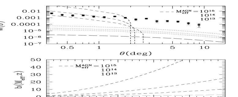
Figure 2: Top panel: contributions to the two-point angular correlation function of NVSS sources with $S_{\rm 1.4GHz}\geq 10$ mJy from AGNs (short-dashed curves), star-forming galaxies (long-dashed curve), and their cross-correlation (dotted curves). The effective halo mass of AGN-powered radio galaxies is assumed to be constant with redshift. The three short-dashed and dotted curves correspond, from bottom to top, to M${}^{\rm AGN}_{\rm eff}=10^{13}$, $10^{14}$ and $10^{15}\,$M_⊙/h, respectively. The effective mass of the halo in which star-forming galaxies reside is M${}^{\rm SF}_{\rm eff}=10^{11}$ M_⊙/h (long-dashed curve). Points with error bars represent the angular two-point correlation function of NVSS sources as measured by Blake $\&$ Wall (2002b). Lower panel: Evolution of the bias parameter for AGNs (short-dashed curves) and star-forming galaxies (long-dashed curves).

As a first step, we obtain estimates of the angular two-point correlation function, $w(\theta)$, assuming a redshift-independent effective mass for the host halos of AGN-powered radio sources, $M^{\rm AGN}_{\rm eff}$, consistent with the clustering properties of optically selected quasars (Porciani, Magliocchetti & Norberg 2004; Croom et al. 2005). The value of $M^{\rm AGN}_{\rm eff}$ is taken as a free parameter. The observationally determined spatial correlation length of star-forming galaxies, $r_{0}(z=0)\sim 3$–4 Mpc/h (Saunders, Rowan-Robinson $\&$ Lawrence 1992; see also Wilman et al. 2003) is consistent with an effective halo mass not exceeding $M^{\rm SF}_{\rm eff}=10^{11}$ $M_{\odot}$/h. We adopt this value in our analysis. Any dependence of $M^{\rm SF}_{\rm eff}$ on redshift can be ignored because of the small range in redshift covered by star-forming galaxies with $S_{\rm 1.4GHz}\geq 10$ mJy.

In the top panel of Fig. 2 we show the contributions to $w(\theta)$ of NVSS sources with $S_{1.4{\rm GHz}}\geq 10\,$mJy arising from the clustering of AGNs with $M^{\rm AGN}_{\rm eff}=10^{13}$, $10^{14}$, and $10^{15}\,M_{\odot}$/h (short-dashed curves) and star-forming galaxies (long-dashed curve), as well as from the cross-correlation between these two populations (dotted curves). As noted above, the cross correlation term, computed from Eq. (7) for the three values of $M^{\rm AGN}_{\rm eff}$, is likely overestimated. The above contributions are then compared with the observational determination of Blake $\&$ Wall (2002b). In the lower panel of the same Figure the redshift-evolution of the bias parameter is represented.

Figure 2 shows that the contribution of star-forming galaxies to the observed angular correlation function is negligible. This is because their contribution to the $S_{\rm 1.4GHz}\geq 10$ mJy counts is small, implying $f_{\rm SF}\sim 5\times 10^{-3}$ [see Eq. (4)], compared with $f_{\rm AGN}\sim 1$. We note that this conclusion is in disagreement with that of Cress $\&$ Kamionkowsky (1998), which relies on the adoption of a local RLF of star-forming galaxies noticeably exceeding the direct estimates of M02.

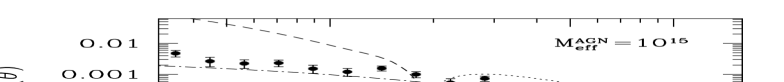
Figure 3: Contributions to the two-point angular correlation function of NVSS sources with $S_{\rm 1.4GHz}\geq 10$ mJy from radio sources above (dashed and dotted lines) and below (dot-dashed line) $z=0.2$, for $M^{\rm AGN}_{\rm eff}=10^{15}\,M_{\odot}$/h and $M^{\rm SF}_{\rm eff}=10^{11}\,M_{\odot}$/h. Star-forming galaxies contribute (yet marginally) only at $z<0.2$. The contribution of higher redshift sources (AGNs only) is positive for $\theta\mathrel{\hbox to0.0pt{\lower 3.0pt\hbox{$\sim$}\hss}\raise 2.0pt\hbox{$<$}}2^{\circ}$, and becomes negative on larger scales (the dotted line shows its absolute values).

Clearly, models in which the mass of the halo hosting AGNs is constant in redshift badly fail at reproducing the overall shape of the observed angular correlation function. This is because contributions to $w_{\rm AGN}(\theta)$ on a given angular scale come from both local and high-redshift sources. For a redshift-independent halo mass, on scales $\theta\mathrel{\hbox to0.0pt{\raise-1.29167pt\hbox{${\scriptstyle\sim}$}\hss}\raise 2.58334pt\hbox{${\scriptstyle>}$}}2^{\circ}$ the positive contribution of local sources is overcome by the negative contribution of distant AGNs, which dominate the redshift distribution and whose bias parameter rapidly increases with redshift [see Eq. (3) and Fig. 2]. In fact, for redshifts $z\mathrel{\hbox to0.0pt{\raise-1.29167pt\hbox{${\scriptstyle\sim}$}\hss}\raise 2.58334pt\hbox{${\scriptstyle>}$}}0.5$–1 such angular scales correspond to distances where $\xi_{\rm AGN}(r)$ is negative.

This situation is illustrated by Fig. 3, showing that the contribution to $w_{\rm AGN}(\theta)$ from local AGNs ($z<0.2$, dot-dashed line) with $M^{\rm AGN}_{\rm eff}=10^{15}\,M_{\odot}$/h comes close to accounting for the observed angular correlation function (the dot-dashed line also includes the contribution of star-forming galaxies with $M^{\rm SF}_{\rm eff}=10^{11}\,M_{\odot}$/h, which however turns out to be almost negligible). But if the same value of $M^{\rm AGN}_{\rm eff}$ also applies to high-redshift AGNs, $w_{\rm AGN}(\theta)$ turns out to be too high on small scales and negative on large scales. Therefore, the only way to account for the behaviour of the data on large scales is to weight down the high-$z$ contribution by decreasing the bias factor at such redshifts. We note that a similar result – which drastically rules out models featuring a bias function strongly increasing with z – was obtained by Magliocchetti et al. (1999) via their counts in cells analysis of the FIRST data.

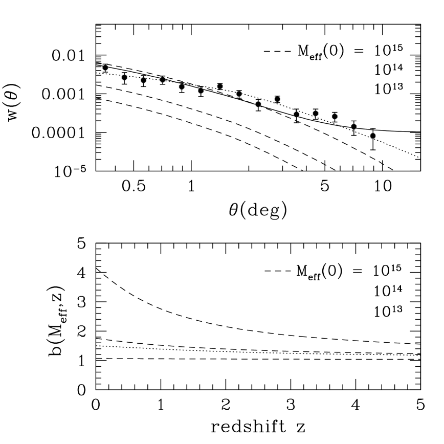
Figure 4: Two-point angular correlation function (top panel), bias parameter (central panel), and effective mass of the host dark matter halo (bottom panel) for radio sources with $S_{1.4\rm GHz}\geq 10\,$mJy for a model in which $M_{\rm eff}\propto M_{\star}(z)$ (see text for details). The three dashed curves correspond, from bottom to top, to different local values of the effective mass: M${}_{\rm eff}(z=0)$ = $10^{13}$, $10^{14}$ and $10^{15}\,M_{\odot}$/h. The solid line in the top panel represents the prediction obtained for $M_{\rm eff}(z=0)=10^{14.9}\,M_{\odot}$/h by adding a constant offset $\epsilon=0.0001$ to $w(\theta)$ in order to account for the effect of possible spurious density gradients in the survey. The dotted curves represent the prediction for $\Omega_{0,m}=0.105$ and $M_{\rm eff}(z=0)=10^{13.15}\,M_{\odot}$/h. Points with error bars show the two-point angular correlation function of NVSS sources as measured by Blake $\&$ Wall (2002b).

Having shown that the contribution of star-forming galaxies to the clustering signal is negligible, hereafter we will only consider AGNs and will drop the ‘AGN’ index from the effective mass.

Based on the fact that AGN-powered radio galaxies are mainly found in very dense environments such as groups or clusters of galaxies, we can then assume that the epoch-dependent effective mass controlling their clustering properties, $M_{\rm eff}$ is proportional to the characteristic mass of virialized systems, $M_{\star}(z)$, which decreases with increasing redshift. $M_{\star}(z)$ is defined by the condition (Mo $\&$ White 1996):

$$\sigma[M_{\star}(z),z]=\delta_{c}(z)$$ (8)

where $\sigma(M,z)$ is the rms fluctuation of the density field at redshift $z$ on a mass scale $M$, while $\delta_{c}(z)$ is the threshold density for collapse of a spherical perturbation at redshift $z$. $M_{\star}$ then represents the typical mass scale at which the matter density fluctuations collapse to form bound structures. As required by the data, this choice for $M_{\rm eff}$ (whose redshift dependence is shown in the bottom panel of Fig. 4) leads to an almost redshift-independent bias factor (central panel of Fig. 4) except for the highest value of $M_{\rm eff}(0)$ for which we have a moderate decrease of $b$ with increasing $z$.

This model successfully reproduces the observed $w(\theta)$ up to scales of at least $\simeq 4^{\circ}$ (top panel of Fig. 4). The best fit is obtained for $M_{\rm eff}(z=0)=10^{14.96\pm 0.04}\,M_{\odot}$/h. On the largest angular scales ($\theta\mathrel{\hbox to0.0pt{\raise-1.29167pt\hbox{${\scriptstyle\sim}$}\hss}\raise 2.58334pt\hbox{${\scriptstyle>}$}}5^{\circ}$), the model correlation function still falls short of the data. However, small systematic variations in the source surface density due to calibration problems at low flux densities may spuriously enhance the estimate of $w(\theta)$ (Blake & Wall 2002a). An offset as small as $\epsilon=10^{-4}$ would be enough to remove the discrepancy between the model and the data (solid line in the top panel of Fig. 4).

On the other hand, if the measured $w(\theta)$ is unaffected by spurious density gradients in the survey, it may be possible to reconcile the model with the observed signal by exploiting the dependence of the model predictions on cosmological parameters, and notably on the matter density parameter, on the baryonic fraction and on the Hubble constant (see Matsubara 2004, Fig. 1). Decreasing $\Omega_{0,m}$ shifts the cut-off of the dark matter spatial correlation function $\xi_{\rm DM}$ to larger scales, while a non-null value of $\Omega_{b}$ determines a peak in the correlation function just below the cut-off scale. The amplitude of this peak is an increasing function of $\Omega_{b}$.

A change in the value of $h$ has an effect which is qualitatively similar to that induced by changing $\Omega_{0,m}$, but of a significantly smaller amplitude; for this reason we have decided to keep this parameter fixed to the reference value $h=0.72$. We have also ignored the dependence of the clustering pattern on the rms mass fluctuation, $\sigma_{8}$: in principle this quantity contributes to the overall normalization of the spatial clustering, but we have checked that in our case the effect of changing it is almost negligible. This is because the decrease of $b$ with increasing $\sigma_{8}$ is compensated by the corresponding increase of the effective mass (assumed to be proportional to $M_{\star}(z)$). Therefore we also keep $\sigma_{8}=0.9$.

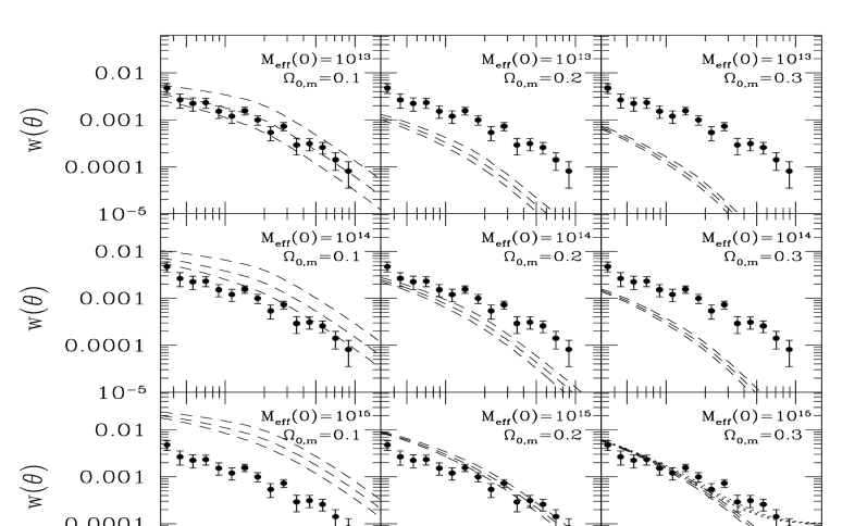
Figure 5: Dependence on cosmological parameters of the two-point angular correlation function of radio sources with $S_{1.4\rm GHz}\geq 10$ mJy. The effective mass of the dark matter haloes in which the sources reside is assumed to be proportional to $M_{\star}(z)$. In each panel, the adopted values of $M_{\rm eff}(0)$ (in solar units) and of the matter density parameter, $\Omega_{0,m}$ are indicated: the former increases from top to bottom panels while the latter increases from left-hand to right-hand panels. In each panel the three dashed curves correspond to different choices for the baryonic mass density parameter: $\Omega_{b}=0.03$, 0.045 and 0.06 from the lower to the upper curves, respectively. In the bottom right-hand panel the dotted curves (almost indistinguishable from each other) represent the two-point correlation function obtained by adding to the dashed curves a constant offset $\epsilon=10^{-4}$ (see text for details).

The parameters in our analysis are then: $M_{\rm eff}(0)$, $\Omega_{0,m}$ and $\Omega_{b}$. In Fig. 5 we show the predicted two-point angular correlation function for different choices of these parameters. In each panel, the dashed curves correspond (from bottom to top) to $\Omega_{b}=0.03$, 0.045 and 0.06. The values adopted for both $M_{\rm eff}(0)$, and $\Omega_{0,m}$ are given in each panel: $M_{\rm eff}(0)$ increases from the top to the bottom panels, while $\Omega_{0,m}$ increases from the left-hand to the right-hand panels.

We note that variations of these parameters within the allowed ranges mainly translate into changes of the normalization of $w(\theta)$, although varying $\Omega_{b}$ also affects the $w(\theta)$ slope on scales $\theta\mathrel{\hbox to0.0pt{\lower 3.0pt\hbox{$\sim$}\hss}\raise 2.0pt\hbox{$<$}}2^{\circ}$, while changes in $\Omega_{0,m}$ modify its slope on larger scales. In general, the amplitude of $w(\theta)$ increases with increasing $M_{\rm eff}(0)$ or $\Omega_{b}$, and decreases for decreasing $\Omega_{0,m}$. From Fig. 5 we can deduce that, given the observed $w(\theta)$, smaller values of $M_{\rm eff}(0)$ are favoured for lower values of $\Omega_{0,m}$.

Fixing the baryonic content to the reference value $\Omega_{b}=0.045$, we have then investigated the $\Omega_{0,m}$–$M_{\rm eff}(0)$ interdependence by constructing $\chi^{2}$ contours on the $\Omega_{0,m}$-$M_{\rm eff}(0)$ plane. The results are shown in Fig. 6 where the curves represent, from the innermost to the outermost, contours corresponding to the 68.3, 95.4 and 99.7 per cent confidence intervals, respectively. The filled square corresponds to the best-fit set of parameters: $\Omega_{0,m}=0.105$, $M_{\rm eff}(z=0)=10^{13.15}\,M_{\odot}$/h. The resulting angular two-point correlation function, and the redshift-evolution of both the bias parameter and the effective mass are represented by the dotted line in Fig. 4. We note that the effect of a change in the baryonic content is just that of smearing the relation between $\Omega_{0,m}$ and $M_{\rm eff}(0)$ (in particular for $\Omega_{0,m}\mathrel{\hbox to0.0pt{\raise-1.29167pt\hbox{${\scriptstyle\sim}$}\hss}\raise 2.58334pt\hbox{${\scriptstyle<}$}}0.2$) since there is a whole set of $\Omega_{0,m}$–$M_{\rm eff}(0)$ pairs which can provide the same best-fit to the data.

Figure 6: Confidence contours derived from a $\chi^{2}$ analysis on the $\Omega_{0,m}$-$\log_{10}[M_{\rm eff}(z=0)]$ plane, having assumed $\Omega_{b}=0.045$. The curves, from inner to outer ones, correspond to the 68.3, 95.4 and 99.7 per cent confidence intervals. The filled square corresponds to the best-fit set of parameters $\Omega_{0,m}=0.105$, $M_{\rm eff}(z=0)=10^{13.15}\,M_{\odot}$/h.

The fit obtained for a zero offset $\epsilon$ is really good, but is obtained for a local matter density parameter $\Omega_{0,m}$ substantially smaller than what indicated by other data sets (see e.g. Spergel et al. 2003), although the difference is significant to less than $3\sigma$. Taken at face value, our results indicate that, within the standard cosmological framework, in the local universe radio sources are as strongly clustered as rich clusters of galaxies, in excellent agreement with the findings of Peacock & Nicholson (1991) and Magliocchetti et al. (2004).

As a last comment, we note that the degeneracy between the host halo mass and the matter density parameter indicates that large area radio surveys without redshift information can hardly provide significant constraints on cosmological parameters, unless independent information on $M_{\rm eff}$ is available. On the other hand, for a given set of cosmological parameters, such surveys yield important information on the masses of the hosting halos.

6 Discussion and Conclusions

The observed angular two-point correlation function of mJy radio sources exhibits the puzzling feature of a power-law behaviour up to very large ($\sim 10^{\circ}$) angular scales. Standard models for clustering, which successfully account for the clustering properties of optically selected quasars, turn out to be unable to explain the long positive tail of the $w(\theta)$, even when ‘extreme’ values for the parameters are invoked. This is because – according to the standard scenario for biased galaxy formation in which extragalactic sources are more strongly clustered at higher redshifts – the clustering signal of radio sources at $z\mathrel{\hbox to0.0pt{\lower 3.0pt\hbox{$\sim$}\hss}\raise 2.0pt\hbox{$>$}}1$, which is negative on large scales, overwhelms that of more local sources, yielding a sharp cut-off in the angular two-point correlation function on scales of $\sim 1$–2 degrees.

The only way out we could find is to invoke the clustering strength of radio sources to be weaker in the past. The data can then be accounted for if we assume that the characteristic mass of the halos in which these objects reside, $M_{\rm eff}(z)$, is proportional to $M_{\star}(z)$, the typical mass-scale at which the matter density fluctuations collapse to form bound structures (see Mo $\&$ White 1996).

A good fit of the observed $w(\theta)$ up to scales of at least $4^{\circ}$ degrees is obtained for $M_{\rm eff}(z=0)=10^{14.96\pm 0.04}\,M_{\odot}$/h. The data on larger scales can be accurately reproduced if the measured values of $w(\theta)$ are slightly enhanced by small systematic variations in the source surface density due to calibration problems at low flux densities (Blake & Wall 2002a). In the absence of such a systematic offset, the data might indicate a lower value of the mean cosmic matter density than indicated by other data sets. The best fit is indeed obtained for $\Omega_{0,m}=0.105$ and $M_{\rm eff}(z=0)=10^{13.15}\,M_{\odot}$/h, with rather large uncertainties on both parameters, as shown by Fig. 6. In particular, the best fit value of $\Omega_{0,m}$ is less than $3\sigma$ away from the ‘concordance’ value. This shows that current large scale radio surveys without redshift measurements cannot provide strong constraints on cosmological parameters, but are informative on the evolution history of the dark matter halos hosting radio sources.

Figure 7: Bias factor as a function of redshift. The data points are from observations of optically selected quasars (open squares from Porciani et al. 2004, filled dots from Croom et al. 2005, open triangle from Grazian et al. 2004; the values of $b$ derived by these authors have been scaled to the values of $\sigma_{8}$ and $\Omega_{0,m}$ used here), while the dashed line represents the functional form derived in this work for the mJy population of radio sources. The dotted curve shows the bias function obtained for a characteristic halo mass constant in time and equal to $\sim 10^{13}\,M_{\odot}$/h.

Taken at face value, the above results point to different evolutionary properties for different types of AGNs as the decreasing trend for the effective mass ruling the clustering of radio sources found in this work strongly differs from the behaviour of that associated to optically selected quasars. For the latter sources, the data are in fact consistent with a constant $M_{\rm eff}\sim 10^{13}\,M_{\odot}$/h, at least up to the highest probed redshift, $z\simeq 2.5$ (see e.g. Grazian et al. 2004; Porciani et al. 2004; Croom et al. 2005) This different behaviour is illustrated in Fig. 7, where the values of the bias inferred for optically selected quasars have been scaled to the values of $\sigma_{8}$ and $\Omega_{0,m}$ used here.

It must be noted, however, that the present data provide very weak constraints on the clustering properties of radio sources at $z\mathrel{\hbox to0.0pt{\lower 3.0pt\hbox{$\sim$}\hss}\raise 2.0pt\hbox{$>$}}1$. For example, we have directly checked that the predicted $w(\theta)$ does not change significantly over the range of angular scales considered here if we assume $M_{\rm eff}\propto M_{\star}(z)$ for $z\mathrel{\hbox to0.0pt{\raise-1.29167pt\hbox{${\scriptstyle\sim}$}\hss}\raise 2.58334pt\hbox{${\scriptstyle<}$}}1.5$ and $M_{\rm eff}\sim{\rm const}\sim 10^{13}\,M_{\odot}$/h at higher redshifts. It is thus possible that the difference in the clustering evolution between AGN-powered radio sources and optically selected quasars is limited to $z\mathrel{\hbox to0.0pt{\lower 3.0pt\hbox{$\sim$}\hss}\raise 2.0pt\hbox{$<$}}1$, consistent with observational indications that, at higher redshifts, the environment of radio-quiet and radio-loud QSOs is almost the same (Russel, Ellison $\&$ Benn 2005).

Interestingly, our analysis indicates that, at $z\simeq 1$, the effective halo mass associated to radio sources is consistent with being essentially equal to that of optical quasars (Croom et al. 2005). This suggests that, at least in this redshift range, the bias parameter for radio-loud and radio-quiet AGNs is similar.

On the other hand, our findings suggest that, at least for $z\mathrel{\hbox to0.0pt{\lower 3.0pt\hbox{$\sim$}\hss}\raise 2.0pt\hbox{$<$}}1$ and at variance with what found for optical quasars, the clustering of radio sources reflects that of the largest halos which collapse at any given cosmic epoch. This conclusion is in keeping with results of previous studies showing that, locally, radio sources are preferentially associated with groups and clusters of galaxies (e.g. Peacock & Nicholson 1991; Magliocchetti et al. 2004), and, at higher redshift, are often associated with very massive galaxies and very massive galaxy environments (e.g. Carilli et al. 1997; Best, Longair $\&$ R$\ddot{\mbox{o}}$ttgering 1998; Venemans et al. 2002; Best et al. 2003; Croft et al. 2005; Overzier et al. 2006).

The major intriguing point that remains unsolved is the link with the population of optical QSOs. The clustering properties of these latter objects seem to reflect that of “normal” elliptical galaxies. So why this difference? Clearly, more observations are crucial to shed light on this issue. So far the main limitation to our understanding of the environmental properties of radio sources has been due to selection effects that allow identifications of mostly radio galaxies in the local universe and exclusively quasars (regardless of their radio activity) at higher redshifts. Therefore, it would be of uttermost importance to consider a redshift range in which the clustering properties of both radio galaxies and radio-active quasars can be measured with good precision. We plan to tackle this issue in a forthcoming paper.

References

- [Becker et al. 1995] Becker R.H., White R.L., Helfand D.J., 1995, ApJ, 450, 559
- [Best 2004] Best P.N., 2004, MNRAS, 351, 70
- [Best et al. 2003] Best P. N., Lehnert M. D., Miley G. K., Rttgering H. J. A., 2003, MNRAS, 343, 1
- [Best et al. 1998] Best P. N., Longair M. S., Rttgering H. J. A., 1998, MNRAS, 295, 549
- [Blake et al. 2004] Blake C., Ferreira P. G., Borrill J., 2004, MNRAS, 351, 923
- [Blake et al. 2004] Blake C., Mauch T., Sadler E.M., 2004, MNRAS, 347, 787
- [Blake Wall 2002] Blake C., Wall J., 2002a, MNRAS, 329, L37
- [Blake Wall 2002] Blake C., Wall J., 2002b, MNRAS, 337, 993
- [Bock et al. 1999] Bock D.C.-J., Large M.I., Sadler E.M., 1999, ApJ, 117, 1578
- [Carilli et al. 1997] Carilli C. L., Rttgering H. J. A., van Ojik R., Miley G. K., van Breugel W. J. M., 1997, ApJS, 109, 1
- [Carroll et al. 1992] Carroll S. M., Press W. H., Turner E. L. 1992, ARAA, 30, 499
- [Condon et al. 1998] Condon J.J., Cotton W.D., Greisen E.W., Yin Q.F., Perley R.A., Taylor G.B., Broderick J.J., 1998, AJ, 115, 1693
- [Cress et al. 1997] Cress C. M., Helfand D. J., Becker R. H., Gregg M. D., White R. L., 1997, ApJ, 473, 7
- [Cress Kamionkowski 1998] Cress C. M., Kamionkowski M., 1998, MNRAS, 297, 486
- [Croft et al. 2005] Croft S., Kurk J., van Breugel W., Stanford S. A., de Vries W., Pentericci L., Rttgering H., 2005, AJ, 130, 867
- [Croom et al2005] Croom S.M., et al., 2005, MNRAS, 356, 415
- [] Daddi, E., Broadhurst, T., Zamorani, G., et al. 2001, A&A, 376 825
- [Dunlop Peacock 1990] Dunlop J.S., Peacock J.A., 1990, MNRAS, 247, 19 (DP90)
- [Eisenstein Hu1998] Eisenstein D.J., Hu W., 1998, ApJ, 496, 605
- [Fanaroff Riley 1974] Fanaroff B.L., Riley J.M, 1974, MNRAS, 167, 31
- [Grazian et al. 2004] Grazian A., Negrello M., Moscardini L., Cristiani S., Haehnelt M. G., Matarrese S., Omizzolo A., Vanzella E., 2004, AJ, 127, 592
- [Ivezic et al. 2002] Ivezi Z. et al., 2002, ApJ, 124, 2364
- [Jackson Wall 1999] Jackson C. A., Wall J. V., 1999, MNRAS, 304, 160
- [Limber 1953] Limber D.N., 1953, ApJ, 117,134
- [Madgwick et al. 2003] Madgwick D. S. et al., 2003, MNRAS, 344, 847
- [Magliocchetti et al. 1998] Magliocchetti M., Maddox S. J., Lahav O., Wall J. V., 1998, MNRAS, 300, 257
- [Magliocchetti et al. 1999] Magliocchetti M., Maddox S. J., Lahav O., Wall J. V., 1999, MNRAS, 306, 943
- [Magliocchetti et al. 2002] Magliocchetti M. et al., 2002, MNRAS, 333, 100 (M02)
- [Magliocchetti et al. 2004] Magliocchetti M. et al., 2004, MNRAS, 350, 1485
- [Matarrese et al. 1997 1997] Matarrese S., Coles P., Lucchin F. Moscardini L., 1997, MNRAS, 286, 115
- [Matsubara 2004] Matsubara T., 2004, ApJ, 615, 573
- [Mo White 1996] Mo H. J., White S. D. M., 1996, MNRAS, 282, 347
- [Moscardini et al. 1998 1998] Moscardini L., Coles P., Lucchin F., Matarrese S., 1998, MNRAS, 299, 95
- [Overzier et al. 2006] Overzier R. A. et al., 2006, astro-ph/0601223
- [Overzier et al. 2003] Overzier R. A., Rttgering H. J. A., Rengelink R. B., Wilman R. J., 2003, AA, 405, 53
- [Peacock Nicholson 1991] Peacock J.A., Nicholson D., 1991, 253, 307
- [Porciani et al. 2004] Porciani C., Magliocchetti M., Norberg P., 2004, MNRAS, 355, 1010
- [Press Schechter 1974] Press W. H., Schechter P., 1974, ApJ, 187, 425
- [Rengelink Rottgering1999] Rengelink R. B., Rttgering H. J. A., 1999, in The Most Distant Radio Galaxies, 399
- [Rengelink et al. 1997] Rengelink R. B., Tang Y., de Bruyn A. G., Miley G. K., Bremer M. N., Rttgering H. J. A., Bremer M. A. R., 1997, AAS, 124, 259
- [\citeauthoryearRicci et al.2004] Ricci R., et al., 2004, MNRAS, 354, 305
- [Rowan-Robinson et al. 1993 1993] Rowan-Robinson M., Benn C. R., Lawrence A., McMahon R. G., Broadhurst T. J., 1993, MNRAS, 263, 123
- [Russel et al. 2005 2005] Russel D. M., Ellison S. L., Benn C. R., 2005, astro-ph/0512210
- [Sadler et al. 2002] Sadler E. M. et al., 2002, MNRAS, 329, 227
- [Saunders et al. 1992] Saunders W., Rowan-Robinson M., Lawrence A., 1992, MNRAS, 258, 134
- [Saunders et al. 1990] Saunders W., Rowan-Robinson M., Lawrence A., Efstathiou G., Kaiser N., Ellis R. S., Frenck C. S., 1990, MNRAS, 242, 318
- [Seldner Peebles 1981] Seldner M., Peebles P. J. E., 1981, MNRAS, 194, 251
- [Shaver Pierre 1989] Shaver P. A., Pierre M., 1989, AA, 220, 35
- [Sheth Tormen 1999] Sheth R. K., Tormen G., 1999, MNRAS, 308, 119
- [Spergel et al. 2003] Spergel D. N. et al. 2003, ApJ, 148, 175
- [\citeauthoryearToffolatti et al.1998] Toffolatti L., Argueso Gomez F., de Zotti G., Mazzei P., Franceschini A., Danese L., Burigana C., 1998, MNRAS, 297, 117
- [Venemans et al. 2002] Venemans B. P. et al., 2002, ApJ, 569, L11
- [Webster 1976] Webster A., 1976, MNRAS, 175, 61
- [Willot et al. 2001] Willot C. J., Rawlings S., Blundell K. M., Lacy M., Eales S. A., 2001, MNRAS, 322, 536
- [Wilman et al. 2003] Wilman R. J., Rttgering H. J. A., Overzier R. A., Jarvis M. J., 2003, MNRAS, 339, 695