Extending the Sensitivity of Air Čerenkov Telescopes

Abstract

Over the last decade, the Imaging Air Čerenkov technique has proven itself to be an extremely powerful means to study very energetic gamma-radiation from a number of astrophysical sources in a regime which is not practically accessible to satellite-based instruments. The further development of this approach in recent years has generally concentrated on increasing the density of camera pixels, increasing the mirror area and using multiple telescopes. Here we present a practical method to substantially improve the sensitivity of Atmospheric Čerenkov Telescopes using wide-field cameras with a relatively course density of photomultiplier tubes. The 2-telescope design considered here is predicted to be more than $\sim$3 times more sensitive than existing/planned arrays in the regime above 300 GeV for continuously emitting sources; up to $\sim$10 times more sensitive for hour-scale emission (relevant for episodic sources, such as AGN); significantly more sensitive in the regime above 10 TeV; and possessing a sky coverage which is roughly an order of magnitude larger than existing instruments. It should be possible to extend this approach for even further improvement in sensitivity and sky coverage.

1 Introduction

The Imaging Atmospheric Čerenkov Telescope (ACT) has proven to be a highly successful technique in the detection of high energy, gamma-rays from astrophysical sources above $\sim$250 GeV. The catalogue of sources so far detected by this ground-based technique includes mainly supernova remnants (SNR) (see e.g. Weekes1989 , Aharonian2001 , Aharonian2005c ) and active galaxies (AGN) (see e.g. Horan2004 and references therein), although recently, new classes of objects such as OB star associations Aharonian2002 and binary systems Aharonian2005a , have been confirmed to be sources of high energy gamma-rays. Also, a recent survey of the galactic plane has yielded a significant signal from the region of the galactic center Aharonian2004a and the discovery of a series of objects lying along the galactic plane Aharonian2005b . The nature of the physics addressed via high energy gamma-ray measurements includes clues to the understanding of the origin of cosmic rays, the nature of AGN jets and the density if the extragalactic infrared background. In addition, several fundamental topics of particle physics can be probed, including searches for TeV-scale WIMP annihilations (see Buckley1998 and references therein), limits on radiative neutrino decay Biller1998 and a fundamental test of Lorentz invariance based on studies of the propagation of very high energy radiation over extragalactic distances Biller1999b . The sensitivities of such searches are among the very best achieved by any technique.

Almost all current ground-based gamma-ray efforts have concentrated primarily on improving the sensitivities to lower energies so as to overlap more with satellite-based observations and potentially map out a larger range of sources. The approaches to this have generally involved increasing the density of camera pixels, increasing the mirror area and using multiple telescopes. However, it is of interest to note that many of the physics topics mentioned above actually stand to benefit most from improved measurements at higher energies. It is in this regime where AGN spectra and short timescale flux variability most critically test acceleration mechanisms as well as uniquely probe the extragalactic infrared background radiation. These higher energy emissions permit the direct study of some of the most extreme and poorly understood environments in the universe. There are now several sources known to produce gamma-ray emission in the regime above 10 TeV, with evidence of some producing gamma-ray emission up to 40 TeV (see e.g. Aharonian2005c ), and potentially as high as 100 TeV Aharonian2004b . Establishing the actual range of this emission would, in itself, be of substantial interest. Furthermore, it is generally acknowledged that much greater sky coverage is desired to study extended sources Aharonian2005c , to better explore the gamma-ray sky and to more continuously monitor multiple sources to study transient behaviour. The approaches so far taken have led to only a modest improvement in this regard, causing many to suggest the need for either a ‘brute force’ use of many tens of telescopes or some “new technology” to allow larger sky coverage at high sensitivity (e.g. ParisConference2005 , Maccarone ).

Our purpose here is to explore a possible method for greatly increasing the sensitivity of ACT instruments using an approach which is practical, economical and does not rely on the development of any new technology Biller2000 . This approach involves the use of cameras with a relatively large field of view, which has the additional advantage of acting as a test-bed for the development of “all-sky” instruments. While initially motivated to improve the sensitivity at higher energies (as in, e.g., Rowell ), the approach is seen to lead to improvements for energies at least as low as 300 GeV. In this present paper, we will develop the basic concept and characteristics of this technique using simulations applied to the case of both a single “Wide Field Of View” telescope (WFOV-1) and a tandem telescope design (WFOV-2). In a later paper, we will extend this approach to a small array and even larger fields of view to explore more details of the range and sensitivity of this approach.

2 The Čerenkov Lateral Distribution of Air Showers and “Wide-field” Imaging

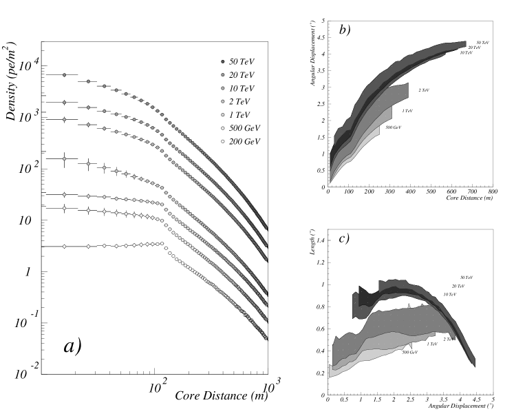
Figure 1: a) Simulated average Čerenkov lateral distribution for showers initiated by gamma-rays of various energies, convolved with atmospheric extinction, mirror reflectivity and typical photomultiplier tube efficiency. All simulated showers were generated from a zenith angle of 0^∘ with an assumed observation level for detection of 2400 m above sea level. b) Image angular displacement ($\mathcal{D}$) as a function of core distance and c) image length ($\mathcal{L}$) as a function of angular displacement for 0.5, 1, 2, 10, 20 and 50 TeV gamma-ray showers. The shaded bands include 68$\%$ of the events about the median. The observed turn-over of the image length distribution for higher energies and larger displacements is due to image truncation by the camera edge (with a radius of $\sim$5^∘).

Extensive air showers induced by primary gamma-rays in the regime near 1 TeV are known to produce a lateral distribution of Čerenkov light at sea level with a relatively constant photon density for distances within $\sim$130 m from the shower core Hillas1996 . By a distance of $\sim$200 m from the core, the density falls by a factor of 2-3 from this value. Consequently, ACTs have generally concentrated on measuring showers landing within the “inner light pool,” where the $\sim$constant photon intensity is at its maximum and its relation to the primary gamma-ray energy is not particularly dependent on a precise knowledge of the core location. This naturally confines the effective areas of individual telescopes to the order of a few times $10^{4}$ m². However, this form of the lateral distribution is also known to change as a function of both detection altitude and primary energy. As an example, figure 1a shows that, for an altitude of 2400 m above sea level and for primary energies of $\sim$2 TeV or more, there is no longer any distinctive plateau at smaller core distances and the density falls in a nearly continuous $\sim$exponential fashion. Therefore, the choice of a fiducial radius for analysis becomes somewhat arbitrary.

If one were to instead base this fiducial radius purely on the observable light level, figure 1a also indicates that the ability of current ACTs to easily trigger for energies of less than 1 TeV would imply that a 10 TeV gamma-ray could be seen beyond a distance of $\sim$500 m. This would correspond to an effective area more than an order of magnitude larger than existing ACTs, and it is this attractive possibility which motivates this present work. Owing to simple geometry, images from showers at larger core distances tend to have an average angle in the camera which is more displaced from the source position. As shown in figure 1b, an image corresponding to a core distance of 500 m would be displaced by approximately 4 degrees. For point-sources tracked in the center of the field of view, this would require a camera with an angular radius of $\sim$5 degrees to contain such images. This raises practical concerns regarding the need to balance this with a large enough density of photomultiplier tubes (PMTs) to adequately define shower image parameters as well as the potential impact of mirror aberrations on such images. On the other hand, as indicated by figure 1c, shower images become elongated by approximately a factor of two at these larger core distances, which should loosen the constraints related to these issues to some extent. Another concern is the need to not only maintain the background rejection capability for large image displacements, but to actually improve it, since lower intensity images will now have to “compete” with a much larger flux of low energy cosmic-ray background showers (mostly due to protons) which bombard the earth from all angles. Finally, there is the question of how well the primary gamma-ray energies corresponding to images with large displacements can be reconstructed.

3 Simulated Configuration

In order to address the issues previously raised, computer simulations were used to investigate the “wide-angle” concept in the context of a practical instrument. The simulation package used Biller1997 was developed based on the EGS4 SLAC and SHOWERSIM Wrotniak codes. The simulated shower development was checked against various analytic treatments and image characteristics were compared both with results from other simulation packages and with actual data from the Whipple imaging ACT Calle2002 . For the purposes of this paper, a baseline telescope configuration was chosen which was similar to that of the Whipple ACT (e.g. Finley2000 ), which has a well-documented history of performance characteristics for a variety of different camera designs and, thus, allows for easy comparison with this device. Accordingly, the model involved a 10 m diameter Davies-Cotton mirror design at an altitude of 2400 m above sea level and wavelength-dependent mirror reflectivity and PMT quantum efficiencies similar to those measured for the Whipple 10 m ACT. However, a slightly longer $f=1$ focal length was used (compared with $f=0.7$), which is more in line with current telescope designs and reduces some of the optical aberrations at large image displacements. Each PMT was modelled with a light concentrator on the front face, possessing a wavelength-independent reflectivity of 80%. The signal recorded in each channel of electronics per event was simply assumed to consist of the earliest detected photon arrival time and the summed number of photoelectrons (pe) for the corresponding PMT.

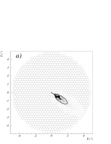
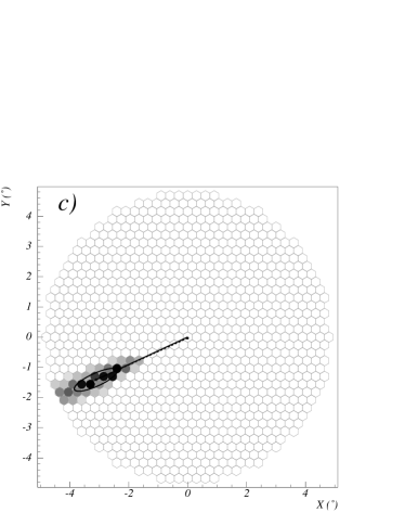
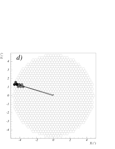
Figure 2: Representative images of simulated 20 TeV gamma-ray showers with increasing distance parameter, going from a), 0.61^∘ through b), 2.44^∘ c), $3.42^{\circ}$ and d), 4.41^∘. Different shaded pixels indicate light intensity.

Based on the previous discussion, the nominal camera design simulated was taken to have an angular radius of 5 degrees, or a full field of view angle of 10 degrees. This is roughly twice the angular diameter of the cameras used for the HESS ACTs Bernlohr2003 and nearly three times those of the VERITAS project Weekes2002 . The cameras for each of these other instruments are composed of an array of PMTs which, individually, have a full field of view angle of $\sim$0.15 degrees. However, as indicated earlier, gamma-ray images corresponding to shower cores which land a few hundred meters away from the ACT are elongated by roughly a factor of two relative to those landing within 100 m (see figure 1c). Hence, it is reasonable to suspect that PMTs with twice the angular acceptance (i.e. 0.3 degrees) might be appropriate for the approach explored here. This would also keep the number of PMTs to less than 1000 per ACT, which is certainly in line with current ACT camera design and couches this study in very practical terms. Consequently, for the purposes of this paper, the nominal simulated camera design consisted of 935 PMTs, each with an angular acceptance of 0.3 degrees, as illustrated in figure 2. Subsequent studies confirmed this PMT density to be sufficient and even suggested it could be somewhat reduced without substantial impact (section 6). We have chosen to model a camera with uniform PMT density (as opposed to one with graded spacing) as it both simplifies image analysis and provides a more uniform sensitivity for sources across the field of view of the instrument. The minimum event trigger conditions required at least any two PMTs in the camera to record a signal in excess of 20 pe above fluctuations in the night sky background, the latter of which was scaled from the recorded data of the Whipple 10 m camera and corresponded to a Gaussian with an RMS of 3 pe for a PMT with a full field of view of 0.25^∘ (15$\mu sr$).

4 Sampling

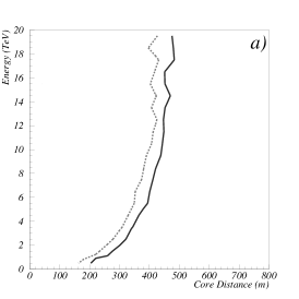
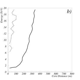
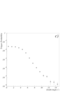
Figure 3: Trigger probability as a function of energy and core distance for simulated gamma-ray events a) and background events b), where the solid line and dashed line indicate the 10$\%$ and 50$\%$ trigger probability contours, respectively, in the case of gamma events, and 10$\%$ and 20$\%$ in the case of background events. c) Trigger probability for proton showers as a function of zenith angle.

In this work, we have concentrated mainly on assessing the performance of the hypothetical instrument to point-sources of gamma-rays and have assumed such a source to be tracked in the center of the field of view of the camera. Table 1 summarises the primary simulation data set used in this work. For simplicity, gamma-ray events have been generated from the zenith, with shower cores randomly sampled over an area on ground within 800 m from the detector. Further increase to the effective area for gamma-rays on the order of a factor of $\sim$3 (though this is energy-dependent) can be achieved when viewing sources at larger zenith angles Petry2001 , but the studies here have been limited to what might be achieved relative to the minimum shower ‘footprint’ from overhead sources. The largest core distance used was chosen to ensure that the probability of triggering the ACT at the highest gamma-ray energies falls to $\sim$zero, so that effective areas can be accurately assessed (figure 3a).

Gamma-rays with energies between 300 GeV and 20 TeV were generated based on a power-law with a differential spectral index of 2.5, which is indicative of many known TeV sources (e.g. Aharonian2001 , Hillas1998 , Aharonian2005d ). A smaller sample of 10 fix energies was also generated for the study of image characteristics at those particular energies. Background images were assumed to be predominantly due to primary proton interactions in the atmosphere, which constitute the majority ($\sim$75%) of cosmic-ray showers that trigger ACTs in the TeV regime. Heavier nuclei are expected to produce shower images which can be rejected at least as easily as those from proton primaries. Images from isolated muons are not explicitly considered in this study as these tend to be readily identifiable for the energy regime considered here. The simulated proton events were generated from a power-law with a differential spectral index of 2.7 Horandel2003 and sampled over the same area on ground as for gamma-ray showers. To insure a reasonable statistical sample in different energy ranges so as to more accurately characterise the nature of these backgrounds in these regimes, proton showers were generated over several, distinct energy intervals with their contributions appropriately weighted to represent the full spectrum. Cosmic-rays are essentially isotropic with respect to the earth, however, in practise, these events can only trigger an ACT within a restricted angular range relative to the telescope orientation. Accordingly, simulated proton-induced background showers were sampled within an angular range of 15 degrees from the telescope axis, which was found to be sufficient (see figure 3c).

To increase the effective statistics, both, gamma-ray and background showers were used 100 times each by sampling the Čerenkov photons over different regions on ground. On average, local variations in the shower properties should be relatively uncorrelated. However, within a given shower, all such sampled densities are correlated with the first few interactions of the primary particle, which determines the height of shower development. Thus, in order to verify that the sampling used did not noticeably bias the results of this study, table 2 compares the average proton and gamma-ray acceptances for different event selection criteria (described below) with the case in which repeated sampling of each shower was not used. As can be seen, there is no evidence of any bias to within the level of the statistical uncertainties of the test. Therefore, repeated sampling was used for increased statistics in order to better study the differential behaviour of the ACT performance. In cases of low statistics in particular parameter regimes, the effect of weighted sampling on the extracted differential behaviour was also directly studied to insure there was no significant bias due to a handful of heavily-weighted showers.

5 Image Analysis

For those images which triggered the detector, we arbitrarily chose to use the same 2-level image cleaning and image parameterisation approach employed by the Whipple group for a camera with a similar individual PMT acceptance (0.25 degrees as opposed to 0.3 degrees) Reynolds1993 . This required a 4.25$\sigma$ signal above sky noise background for “picture” pixels and 2.25$\sigma$ for neighbouring “boundary” pixels. In addition, to ensure that enough information was available to reconstruct the image parameters reliably, accepted images were required to have at least 5 picture pixels.

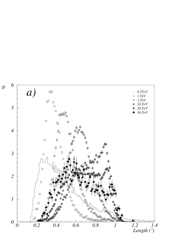
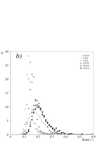
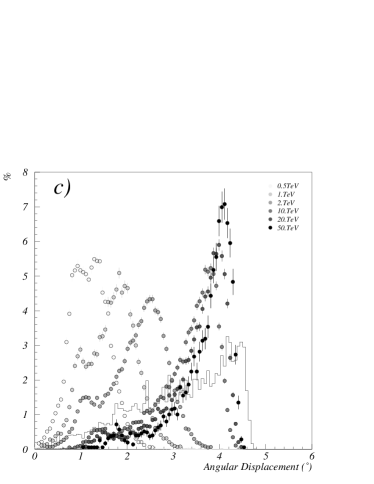
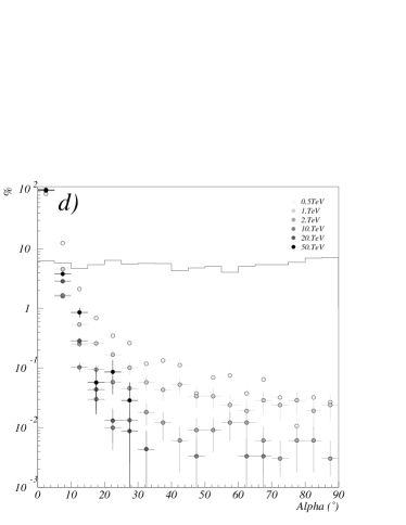
Figure 4: Image parameter distributions for simulated triggering gamma-ray events of 6 different energies (not normalised according to spectral shape) and background events summed over all energies (see table 1).

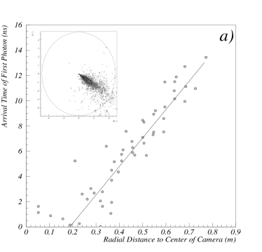
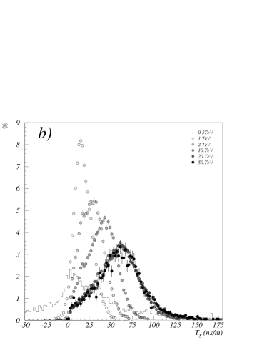
Figure 5: a) Arrival photon time on the camera for a simulated gamma-ray event. Each point in the graph corresponds to the arrival time of the first photon at a particular PMT. Only image pixel are used to derive the slope, $\mathcal{T}_{S}$. The corresponding gamma-ray image is shown in the in-set figure. b) Distribution of $\mathcal{T}_{S}$ for simulated triggering gamma-ray images of different 6 energies (not normalised to account for spectral shape). The continuous line is the equivalent distribution of $\mathcal{T}_{S}$ for simulated background events summed over all energies (see table 1).

Images were then analysed in terms of moments according to the Hillas prescription Hillas1985 . The relevant image parameters used in this study were: 1) the summed number of detected photoelectrons in the image, $\mathcal{S}$; 2) the average angular displacement in the camera relative to the source position, $\mathcal{D}$; 3) the mean length of the image, as measured along its major axis, $\mathcal{L}$; 4) the mean width of the image, as measured along its minor axis, $\mathcal{W}$; and 5) the angle of the major axis with respect to the line linking the image centroid with the assumed source position, $\alpha$. All of these parameters were couched in units of degrees. Figure 4 shows the distributions of these image parameters for gamma-ray and background events. In addition, a further image parameter, $\mathcal{T}_{S}$, was defined as the slope extracted from a linear fit to the earliest photon arrival time in each PMT as a function of the angular distance of that PMT from the assumed source position. This characterises the projection of distances to Čerenkov-emitting regions along the axis of shower development, given the expected primary gamma-ray direction. Figure 5 illustrates the definition of $\mathcal{T}_{S}$ for a particular event.

6 Dependence on Pixel Size

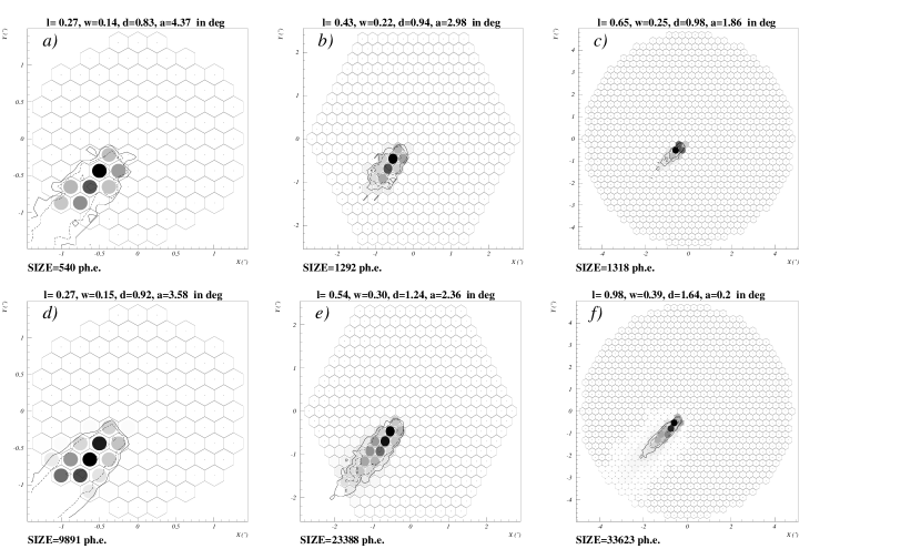
Figure 7: Simulated 1 TeV gamma-ray event at d_core=120 m (top panel), and 20 TeV gamma-ray event at d_core=120 m (bottom panel) as recorded by cameras with different field-of-view (FOV). From left to right, $\sim 3^{\circ}$, $\sim 5^{\circ}$ and $\sim 10^{\circ}$ FOV. The first two are similar in FOV to Whipple cameras and the third one, corresponds to the wide field of view camera used in the simulations presented in this work. Note as well that the pixel size is different for each camera (from left to right, $\sim 0.19^{\circ}$, $\sim 0.23^{\circ}$ and $\sim 0.3^{\circ}$ FOV). Superimposed on top of the shower images are 5% (outer line), 10%, 50% and 90% photon density contours.

The impact of pixel size (PMT density) on ACT sensitivity enters primarily though the ability to characterise image shape and orientation so as to aid in background rejection. Consequently, we have explored the ability to reconstruct the parameters $\mathcal{L}$, $\mathcal{W}$ and $\alpha$ as a function of $\mathcal{D}$ for simulated cameras corresponding to pixel sizes of 0.22, 0.3, 0.4 and 0.82 degrees in diameter. These were also compared with values from actual Whipple and VERITAS data for cameras with various pixel sizes over their limited range in $\mathcal{D}$. The results are shown in figure 6. Several characteristics are worth noting: 1) The ability to determine image orientation ($\alpha$) is substantially improved at larger image displacements. 2) The ability to characterise image parameters is noticeably improved for pixel sizes of 0.4^∘ compared to 0.8^∘, but any further improvement from using even smaller pixels is relatively modest. This is consistent with the findings of Aharonian et al. Aharonian1995 . 3) The fact that very small pixel sizes even appear to do worse in determining $\alpha$ at larger image displacements is an artifact of trigger selection owing to the decreasing photon levels in smaller PMTs and the specific trigger requirements assumed. 4) Data from actual ACTs seem to have generally larger values of $\alpha$ in the angular displacement range of $\sim$1^∘ than is predicted by the simulation. Once more, this appears to be largely due to the field of view and the fact that smaller cameras tend to truncate more of the outer parts of these images. This effect is illustrated in figure 7, in which comparisons are made with simulations using different fields of view.

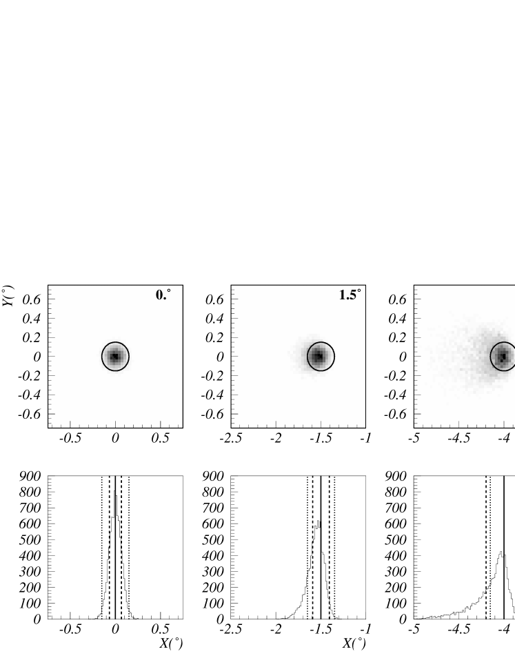
Figure 8: Distribution of photons on the camera plane for an on-axis point source and for two different off-set positions, 1.5^∘ and 4.^∘. The circle corresponds to the individual PMT area. The solid lines in the three bottom plots indicate the expected peak position, the dashed lines are the 1 $\sigma$ region along the radial direction ($\sigma_{r}$) and the dotted lines indicate the PMT size.

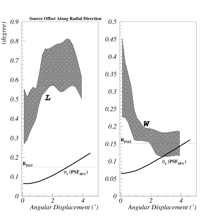
Figure 9: a) RMS of the PSF ($\sigma_{r}$) along the radial direction for different source offset positions. The shaded region includes 68$\%$ of the events about the median length, $\mathcal{L}$, as a function of radial distance for a subset of simulated 2 TeV gamma-ray showers. b) Similar plot for the RMS of the PSF along the angular direction ($\sigma_{\phi}$), where the shaded region includes 68$\%$ of the events about the median width, $\mathcal{W}$, for the same showers.

In addition, the Point Spread Function (PSF) of the detector due to mirror aberrations, has been calculated as a function of the source offset angle (figure 8). Figure 9 shows the PSF together with the median length ($\mathcal{L}$) and width ($\mathcal{W}$) as a function of the angular displacement ($\mathcal{D}$). The figure indicates that the PSF should not affect the ability to reconstuction the image angular size.

Based on the above studies, the choice of the 0.3^∘ pixel size used to explore the wide-field concept in this current paper would appear to be more than adequate. Indeed, it is likely that a camera with even larger pixels could be used without significantly affecting the performance of the instrument.

7 Single Telescope Performance

We will first consider a single, isolated, wide-angle telescope and assess its performance in terms of background rejection, energy resolution, and effective area. Based on this, the sensitivity of the instrument to a hypothetical point-source will be estimated for both long term (50 hours) and short term (1 hour) observation periods, which will be compared with that of other ACT instruments.

7.1 Image Selection Criteria

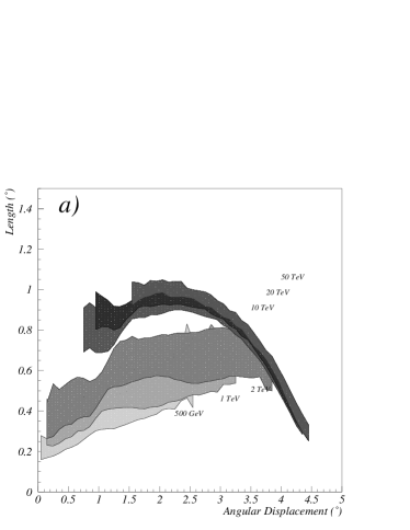
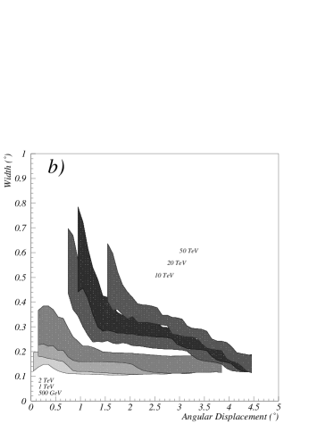
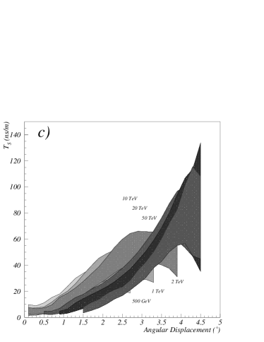
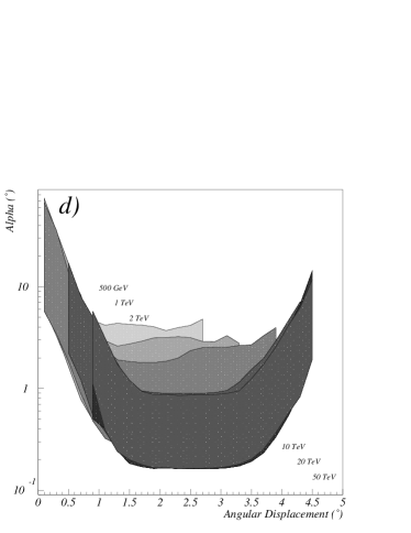
Figure 10: Image parameters as a function of angular displacement on the camera for triggering gamma-ray showers of 6 different energies. The shaded regions include 68$\%$ of the events about the median.

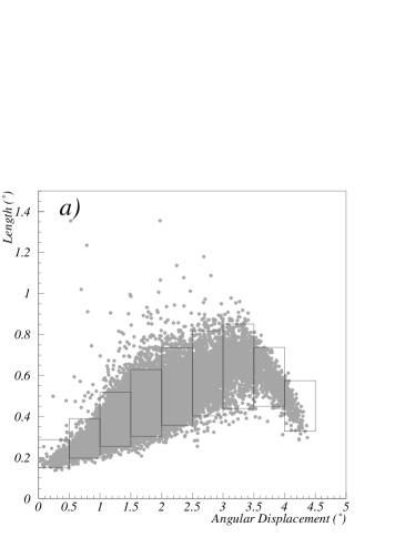
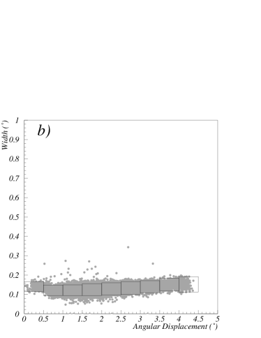
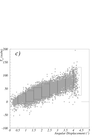
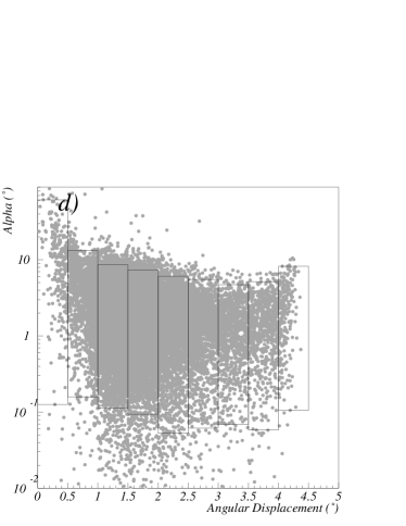
Figure 12: Acceptance intervals for each of four image parameters used in this work for background rejection as a function of angular displacement, $\mathcal{D}$, for a given range in $\log_{10}(\mathcal{S}$). The dots correspond to individual gamma-ray images. The width of each box indicates the angular displacement interval over which median values are obtained (see text for details), while the length of the box corresponds to the 95$\%$ acceptance interval about the median.

In the approach followed here, the goal is to attain good background rejection without sacrificing collection area for events over a large range of energies and core distances from the ACT. These latter properties are most directly related to the parameters $\mathcal{S}$ and $\mathcal{D}$. Figures 10 and 11 show the image parameter distribution as a function of angular displacement ($\mathcal{D}$) for gamma-ray and background events respectively. Hence, simulated gamma-ray images were first categorised into 10 intervals of $\mathcal{D}$ (each spanning 0.5^∘) and 20 logarithmic intervals in $\mathcal{S}$ (each spanning 0.5 in log10($\mathcal{S}$)). For each division defined by the resulting 2-D matrix, symmetric acceptance intervals about the median of each of the remaining image parameters were defined so as to arbitrarily contain 95% of the gamma-ray images. Figure 12 illustrates the definition of image selection for events within a given log10($\mathcal{S}$) interval. The intervals for the parameters $\mathcal{L}$ and $\mathcal{W}$ define images which have shapes typical of gamma-ray images, whereas the intervals corresponding to $\alpha$ and $\mathcal{T}_{S}$ define images whose orientation is characteristic of a primary which came from the assumed source position. In particular, $\alpha$ is related to the angular resolution and $\mathcal{T}_{S}$ characterises the extent to which the value of $\mathcal{D}$ is due to the displacement of the shower core as opposed to a nearby shower with a larger relative inclination angle which, therefore, is not associated with the source. In addition, $\mathcal{T}_{S}$ was required to be positive in order to remove low energy events landing very near the detector for which the value of $\mathcal{T}_{S}$ is poorly defined. Table 2 shows the efficiency of each one of the acceptance cuts individually applied to independent simulated gamma-ray and proton spectra. From this, it can be seen that the introduction of $\mathcal{T}_{S}$ yields an extra factor of between 2 and 3 in background rejection.

7.2 Shower Core and Energy Resolutions

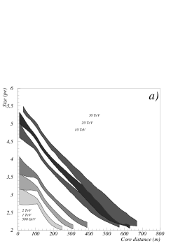
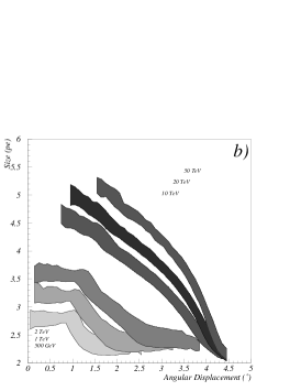
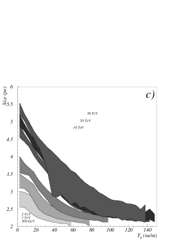
Figure 13: Image size, $\mathcal{S}$, as a function of a) core distance b) angular displacement $\mathcal{D}$ and c) $\mathcal{T}_{S}$ for gamma-ray showers of 6 different energies. The shaded regions include 68$\%$ of the events about the median.

A $\chi^{2}$ minimisation method was employed to simultaneously reconstruct the core position and gamma-ray energy of each event so as to explore resolution properties of the hypothetical ACT. This approach also has the advantage of being trivially extended for use with multiple telescopes, which will be explored in section 8. Three image characteristics were used in this fit (see figures 13 and 14): $\mathcal{D}$, $\log_{10}(\mathcal{S}$) and $\log_{10}(\mathcal{T}_{S}/\mathcal{D}$). The factor of $\mathcal{D}$ in the latter expression removes the first-order dependence on this parameter and allows the $\chi^{2}$ to be better approximated by a linear sum of independent contributions from each of these characteristics. To define the $\chi^{2}$ model, simulated gamma-ray events were first categorised into 10 m intervals of core distance and logarithmic intervals of primary gamma-ray energy using 4 bins per decade. The model was extended in energy, with respect to our standard data set (table 1), down to 30 GeV and up to 55 TeV to reduce reconstruction biases for events near the boundaries of this set. For each division of this 2-D matrix, the median value of each image characteristic was determined, along with “equivalent” upper and lower one standard deviation values, defined as those values which bound $\pm$34% of images about this median. The $\chi^{2}$ function was then defined as:

$$\chi^{2}\equiv\sum_{i=1}^{3}\left[\frac{m_{i}-m_{i}^{0}(E,R)}{\sigma_{i}^{0}(E,R)}\right]^{2}$$

where $m_{i}$ is the measured median value of the $i$th image characteristic for the event; and $m_{i}^{0}(E,R)$ and $\sigma_{i}^{0}(E,R)$ are the model predictions for the median and effective standard deviation for this characteristic, respectively, as a function of primary energy, $E$, and distance from the shower core, $R$. Appropriate $\sigma_{i}^{0}(E,R)$ values were used depending on whether the $m_{i}$ was above or below $m_{i}^{0}(E,R)$

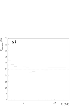
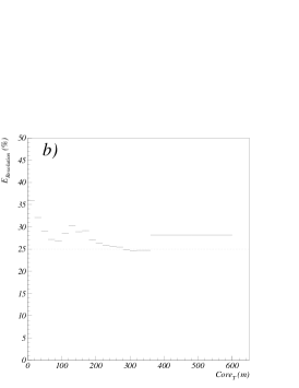
Figure 16: RMS energy and Core resolution as a function of true energy (E_T) and true core distance (Core_T) for a single wide-angle telescope.

Using an independent simulated data set (300 GeV-20 TeV) from that used to generate the model (30 GeV-55 TeV), this $\chi^{2}$ was then minimised with respect to $E$ and $R$ for each event, using values from the 2-D matrix described above. Despite the approximations of independent image characteristics and normal errors, the resulting distribution of $\chi^{2}$, shown in figure 15, is in reasonable agreement with the expected 1 degree of freedom. To remove poorly defined images, those events with values of the $\chi^{2}$ probabilities less than 10% were eliminated from the data set as well as those with reconstructed energies outside the considered energy range 300 GeV-20 TeV. Together, these cuts remove $\sim$27% of the gamma-ray events that passed image cuts and $\sim$66% of proton events. Based on this procedure, figure 16 shows the derived core and energy resolutions as a function of actual primary gamma-ray energy and true core distance from the ACT. For a single telescope, an energy resolution of $\sim$25% is achieved above 1 TeV, essentially independent of the core distance.

7.3 Effective Areas

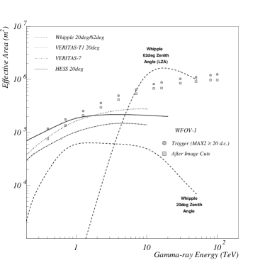
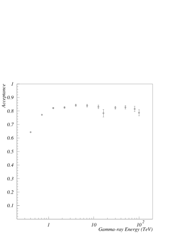
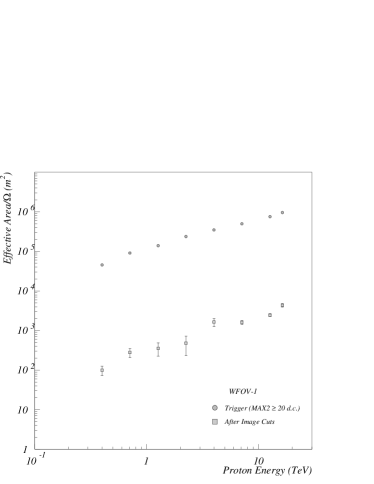
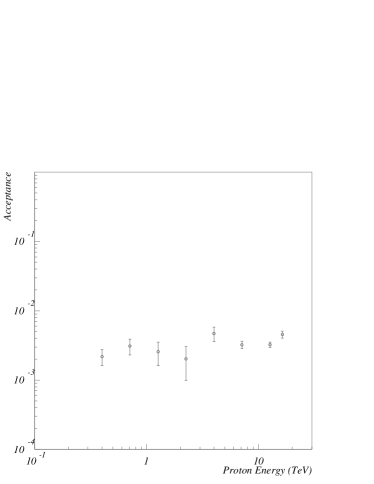
Figure 17: a) Gamma-ray collection areas, both at the trigger level and after image cuts, for a single wide-angle camera (WFOV-1). The different lines correspond to effective areas after image cuts for Whipple-490 and Whipple-490 at Large Zenith Angle (LZA) Petry2001 (dashed line), HESS Benbow2005 (continuous line) and VERITAS-T1 Maier2005 (dotted line), VERITAS-7 Weekes2002 (dotted-dashed line). b) Gamma-ray acceptance as a function of energy. c) Background collection areas, both at the trigger level and after image cuts, for a single wide-angle camera (WFOV-1). The collection area for protons has been normalised to the solid angle subtended by the camera. d) Background acceptance as a function of energy.

The “effective area” for a given class of events was computed as the projected area on the ground over which simulated core locations are uniformly sampled with respect to the ACT, times the fraction of such events which are retained in the data sample. Figure 17 shows the derived effective areas for gamma-ray and proton showers as a function of the true primary energy for triggered showers both before and after image selection. As expected, approximately $(0.95)^{4}\sim$80% of gamma-ray images are retained after selection based on the 4 image parameters. The effective collection area for gamma-rays after this selection is $\sim 2\times 10^{5}$ m² at primary energies of 1 TeV and exceeds $\sim 5\times 10^{5}$ m² above 5 TeV. This is roughly an order of magnitude larger than a conventional, single telescope and about twice that of the HESS or VERITAS arrays. At higher energies, the relative gain in effective area is even greater.

For proton-induced showers, the effective collection areas are suppressed by roughly a factor of $10^{3}$ following image selection. However, it should be noted that background rejection factors cannot be directly implied from these figures since the true primary energy is not an observable. Thus, the resolution of “equivalent” gamma-ray energies and their effect on assumed background and source spectra must be taken into consideration.

The raw trigger rate from background showers based on an assumed proton flux of $\Phi_{p}(E)=8.73\times 10^{-2}E_{TeV}^{-2.7}$ m^-2 s^-1 sr^-1 TeV^-1 Horandel2003 , is found to be $\sim 1~{}kHz$, using the basic trigger scheme assumed here. A simple pattern trigger can further reduce this by a factor of $\sim$2 Bradbury1999 , making it easily manageable by relatively standard data acquisition electronics (see e.g. Funk2004 ).

7.4 Single Telescope Flux Sensitivity

The image selection and energy reconstruction procedures previously described were applied to simulated proton and gamma-ray spectra sampled from differential power laws of the form $E^{-2.7}$ and $E^{-2.5}$, respectively. In order to couch the derived quantities in terms of typical detection rates, the simulated spectra were initially normalised according to $\Phi_{p}(E)=8.73\times 10^{-2}E_{TeV}^{-2.7}$  m^-2 s^-1 sr^-1 TeV^-1, based on cosmic ray primary measurements Horandel2003 ; and $J_{\gamma}(E)=3.2\times 10^{-7}E_{TeV}^{-2.5}$  m^-2 s^-1 TeV^-1, based on the measured high energy flux from the Crab Nebula near 1 TeV Hillas1998 . These were then convolved with the relevant effective collection areas and used to yield differential detection rates in terms of the reconstructed, effective gamma-ray energy, $E^{\gamma}_{Rec}$. These are shown in figure 18, for different ranges of $\mathcal{D}$.

These figures may be used to derive the detector “sensitivity” for such a source spectrum by first integrating the rates over a chosen time scale, then scaling the assumed gamma-ray flux until a given minimum significance level for detection over some defined effective energy range is reached. For the purposes of this paper, the sensitivity will be defined based on the integrated signal above a given effective energy threshold which yields a detection at a significance level of 5$\sigma$ and a minimum of 10 detected high-energy gamma-rays. It will also be assumed that the nominal background rate is well known. In practise, uncertainties in this background rate will reduce the significance level to some extent, so that the curves derived here may be more indicative of detection levels corresponding to $\sim$3-4$\sigma$.

Particularly for this type of camera, background levels will be highly dependent on both the reconstructed gamma-ray energy and the apparent core distance. To account for this, the average signal and background levels were first computed separately for the 3 regions of $\mathcal{D}$ shown in figure 18 (0-2.6^∘, 2.6^∘-3.7^∘ and 3.7^∘-4.5^∘) and in each of 8 logarithmic energy intervals between 300 GeV and 20 TeV. A maximum likelihood ratio, $L_{r}$, was then constructed relative to the zero-signal case. $-2logL_{r}$ is approximately distributed as a $\chi^{2}$ distribution Wilks1938 , from which the average detection significance was calculated assuming that three variable parameters of signal strength, power-law index and spectral cut-off may be fit to the data. This approach appropriately weights the contributions from the different signal/background regimes.

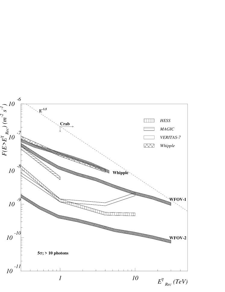
Figure 19: Integral sensitivity curve for a 50 h exposure for the detectors simulated in this work assuming an integral $E^{-1.5}$ source spectrum. WFOV-1 refers to a single detector while WFOV-2 refers to the tandem telescope configuration described in the text. Also shown is the sensitivity curve for a Whipple-like detector derived using the same simulation software used to explore the wide-angle telescope considered in this work. These are compared with the stated sensitivity curves for other experiments from Weekes2002 and Hofmann2001 .

The resulting sensitivity curves as a function of $E^{\gamma}_{Rec}$ are shown in figures 19 and 20 for exposure times of 50 hours and 1 hour, respectively. These are compared with similar curves for the Whipple, MAGIC, VERITAS and HESS instruments, taken from Weekes2002 and Hofmann2001 . To verify the consistency of the methods used to obtain the following results, the sensitivity of the Whipple telescope was also independently estimated for 50 hours exposure time using the same simulation software and similar analysis procedure as employed for the wide-angle camera study. As can be seen in figure 19, the results are in excellent agreement with published values.

For continuous sources based on 50 hours of exposure, the wide-angle camera is found to be approximately a factor of two more sensitive than the Whipple instrument, even at energies as low as 300 GeV. This stems from the fact that, even at these low energies, the collection area for the larger field of view is roughly a factor of two larger than the Whipple instrument and the $\mathcal{T}_{S}$ selection (made more effective by the larger field of view) suppresses the background by an addition factor of $\sim$2. As the sensitivity is proportional to the square root of both these factors, the overall improvement in sensitivity by a factor of two is as expected.

For this same exposure, the device becomes comparable to VERITAS and HESS at energies above 10 TeV, despite backgrounds, owing to the greatly increased collection area. For studies based on 1 hour of exposure (as might be characteristic of transient emission from AGN), the wide-angle camera surpasses the sensitivity of the arrays above 2-3 TeV, despite being only a single telescope with a $\sim$30% smaller mirror area than each element of the arrays. This is due to the fact that, with it’s much larger collection area, the wide-angle camera tends to be background dominated rather than statistics limited. Thus, any decrease in the relative background level (whether through improved background rejection or higher source fluxes over shorter exposure times) results in greater improvement relative to conventional cameras, which become starved for signal above $\sim$1 TeV (as indicated by the upwards turn in their sensitivity curves in figure 20).

8 Tandem Telescope Configuration

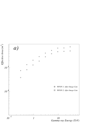
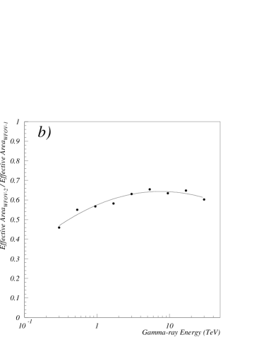
Figure 21: a) Comparison of the gamma-ray collection areas (after image cuts) of a single wide-angle camera detector (WFOV-1) and the tandem telescope configuration (WFOV-2) simulated on this work. b) Ratio of these effective areas.

Background rejection is clearly a key factor to instrumental sensitivity. This is particularly true for the wide-field concept, which seeks to extend the dynamic range by essentially swapping a statistically limited regime for one which is more background limited, as previously mentioned. One obvious way to gain further background rejection and also improved energy resolution is with the use of multiple telescopes. In order to explore the potential gain in sensitivity by this approach, we have limited our consideration here to a tandem configuration in which identical wide-field ACTs are separated by 125 m, which is close to the optimum distance suggested by Aharonian et al. based on trigger rates Aharonian1997 . However, note that we have not specifically optimised this configuration in terms of background rejection versus effective collection area for the instrument considered here, but have only chosen this as a “representative” configuration to explore the basic characteristics. We have also not optimised the trigger for a 2-telescope system, but have simply imposed the same single telescope trigger and image analysis/rejection previously described to both cameras (figure 21). The simulated data set used for this study is summarised in table 3. As with the case of protons in the previous study, showers were generated over several different energy intervals and joined via an appropriate weighting to represent full spectra so as to improve the statistical characterisation in very different energy regimes.

8.1 Tandem Shower Core and Energy Resolution

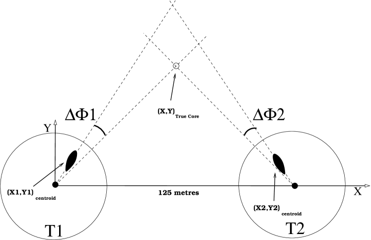
Figure 22: Illustration of the model parameter $\Delta\Phi$ used for core reconstruction with the tandem telescope configuration.

The $\chi^{2}$ approach for determining primary energy and core location was modified for the 2-telescope case to simultaneously fit both camera images. This was done by fitting for the 2-dimensional core location (as opposed to simply radius) and introducing a 4th image characteristic, $\Delta\Phi$, which is sensitive to the angular orientation of the core with respect to the coordinates of each telescope. This parameter was defined as the angular deviation between the core direction and the direction of the image centroid, both relative to the centre of the particular camera (which is assumed to track the source). This definition is illustrated in figure 22. Thus, the $\chi^{2}$ function for the “jth” telescope becomes:

$$\chi^{2}_{j}\equiv\sum_{i=1}^{4}\left[\frac{m_{i}-m_{i}^{0}(E,R)}{\sigma_{i}^{0}(E,R)}\right]^{2}$$

where the sum is over each of the 4 image parameters. The overall $\chi^{2}$ function for an array of $n$ telescopes is therefore:

$$\chi^{2}_{array}=\sum_{j=1}^{n}\chi^{2}_{j}$$

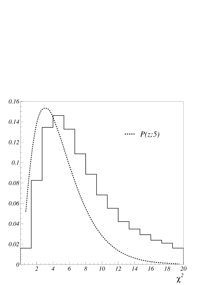
Figure 23: $\chi^{2}$ distribution of reconstructed tandem-telescope events. Only events which energy falls in the 300 GeV-20 TeV energy range are represented here. The dashed line is the probability density function for the $\chi^{2}$ distribution with 5 degrees of freedom.

Given the three free fit parameters (the 2-D core location plus primary gamma-ray energy), for the case of 2 telescopes (each involving 4 measured characteristics), this should nominally correspond to 5 degrees of freedom. However, this once more assumes that the image characteristics are completely uncorrelated and that the uncertainties are normally distributed, neither of which is strictly true. The actual $\chi^{2}$ distribution is compared with the idealised case in figure 23.

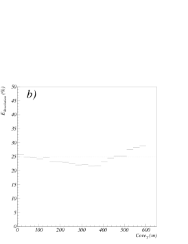
Figure 24: RMS energy and Core resolution as a function of true energy (E_T) and true core distance (Core_T) for the tandem telescope configuration.

In applying this fitting procedure to simulated data, as in the case of a single telescope, events with values of $\mathcal{D}$ greater than 4.5^∘ or fit $\chi^{2}$ values less than 10% likely were eliminated from the data set in order to remove poorly defined images. Figure 24 shows the derived core and energy resolutions as a function of actual primary gamma-ray energy and true core distance from the ACT. An energy resolution of $\sim$20% is achieved, as compared to the single telescope value of $\sim$25%.

8.2 Inter-Telescope Timing and Shower Maximum

The relative arrival times of the Čerenkov signal in different telescopes can also provide valuable information. The thickness of the Čerenkov wavefront from an extensive air shower is expected to be $\sim$5-10 ns and the Davies-Cotton design considered here results in light paths to the camera which differ by as much as 5 ns. However, a typical gamma-ray image involves several hundred photoelectrons, such that the statistical sampling should allow a sub-nanosecond measurement of the relative wavefront arrival time. For an array of telescopes spread over a baseline of $\sim$100-200 m, this alone could provide a determination of the shower arrival direction with an accuracy comparable to or better than that based on image orientation. However, even for the case of two telescopes explored here, the relative arrival times of the Čerenkov signal can be combined with the reconstructed shower core position to yield information on the height of shower maximum and also provide another useful discriminant against background showers.

In particular, if it is assumed that the Čerenkov light is emitted from a height of maximum shower development, $h_{max}$, above the detector level, for the simple case here in which the source is at zenith, the time at which the telescope receives the light is then just given by:

$$t=\frac{n}{c}\sqrt{h_{max}^{2}+R^{2}}$$

where n is the refractive index of air and $R$ is the distance from that telescope to the shower core at the detection level. Thus, in the limit where $h_{max}\gg R$ and $n=1.0$, the difference in time between two different telescope measurements is given by:

$$\Delta t\simeq\frac{1}{2ch_{max}}(R_{2}^{2}-R_{1}^{2})$$

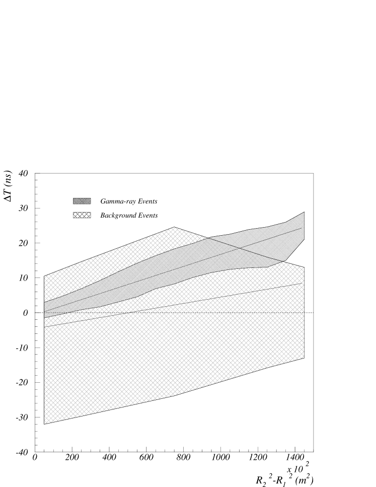
Figure 25: Relative shower arrival time as a function of relative squared distance to the shower core to the different telescopes. The dark-shaded band corresponds to the 95$\%$ gamma-ray events which have passed image selection. The light-shaded band is the equivalent for background events, where only events which have passed the trigger condition and have at least 5 picture pixels and $\mathcal{T}_{S}\geq 0.$ are represented.

Thus, a plot of $\Delta t$ versus $(R_{2}^{2}-R_{1}^{2})$ should yield a well-defined linear relation for gamma-rays, whose slope is proportional to the height of shower maximum (figure 25). In practise, the lateral extent of the gamma-ray shower at the point of maximum development means that much of the light arrives from distances somewhat closer to the detector than is implied by the shower core. This causes the apparent $h_{max}$ derived from the simplistic expression above to be overestimated. In order to apply this to a simulated data set, the reconstructed core locations were used (as previously described) and the relative “image time” in each telescope was defined as that of the image centroid, using the linear fit parameters derived in the determination of $\mathcal{T}_{S}$. Results are shown in figure 25 for a simulated gamma-ray source.

A selection criteria based on this to discriminate against background was formed by defining a range of $\Delta t$ as a function of $(R_{2}^{2}-R_{1}^{2})$ which contains 95% of the gamma-rays. This was found to reject $\sim$85% of proton events which would otherwise pass data selection.

8.3 Factorised Background Rejection

The very large background rejection associated with a multi-telescope system can impose statistical limitations on the ability to extract detailed information about the behaviour of the expected background from a finite set of simulations. However, many of the image selection criteria are independent of each other to a very large extent, thus allowing their individual effects to be well determined and then combined as a product. To explicitly verify this approach for the current case, we first consider the background rejection of a single camera for proton events which have triggered both telescopes and pass the selections $\mathcal{D}<4.5^{\circ}$, $\mathcal{T}_{S}>0$ and npicture $\geq$ 5. Table 5 shows the fraction of such events which pass different data selection criteria, both individually and in various combinations. These numbers indicate that selections based on 1) image shape ($\mathcal{L}$ and $\mathcal{W}$), 2) image orientation $\alpha$, and 3) $h_{max}$, based on relative image times (in this case making use of information from the second telescope), are all largely independent of each other.

We now consider these data selection criteria applied to the case of two telescopes. While the effect of any given selection is generally correlated between both cameras, the joint application of each selection will still be independent from the joint application of another selection. Table 6 lists the two-telescope proton rejection factors for each the three selections listed above.

Furthermore, the effect of a selection based on the $\chi^{2}$ goodness of fit to the gamma-ray energy and core location can also be separately applied as a factor since the parameters involved ($\mathcal{S}$, $\mathcal{D}$ and $\mathcal{T}_{S}$) are independent of the three selections above: Image shape and orientation selections are parameterised as a function of $\mathcal{S}$ and $\mathcal{D}$ to explicitly remove any dependence, while the relative image times are, by construction, independent of individual telescope time measurements. For the case of two telescopes, a $\chi^{2}$ selection chosen to keep 90% of gamma-ray images was found to reject $\sim$85% of proton shower images.

The combination of these factors for the case of two-telescope analysis is shown in table 6 for 2 different ranges of reconstructed gamma-ray energy. As no clear dependence on this reconstructed energy is seen, a single, average rejection factor will be applied to scale the detection rates from the one telescope to the two telescope case.

8.4 Tandem Telescope Sensitivity

Following a similar procedure to that employed for a single telescope, figures 19 and 20 show the sensitivity of a tandem, wide-angle instrument to a hypothetical point-source with an $E^{-2.5}$ differential spectrum, both for 50 hours and 1 hour exposure times, respectively. This is compared with similar curves for the VERITAS/HESS instruments. The scaling relative to the single telescope case is consistent with the factor expected from comparing the Whipple with the VERITAS/HESS sensitivities Weekes2002 (figure 19), with an additional factor of $\sim$2 gained from the $h_{max}$ selection. For the 50 hour exposure, the sensitivity of the tandem wide-angle design is a factor of $\sim$4 times more sensitive over the range above 300 GeV, with extended sensitivity above 10 TeV. For the case of 1 hour exposure, the sensitivities are comparable at 300 GeV and exceed an order of magnitude improvement in sensitivity above 5 TeV.

9 Summary and Conclusions

The study presented here suggests that the sensitivity of ACT instruments could be substantially improved in the regime above 300 GeV through the use of cameras with much larger fields of view for the same PMT density than are currently employed. Particularly for the tandem telescope design considered in this paper, the ability to image showers further “off-axis” leads to a significant gain in effective area with no significant loss in energy resolution compared with current instruments, even for showers with cores landing much further from the telescopes. The ability to suppress background events also appears to be substantial for such a design and yields a very good sensitivity over a remarkably large dynamic range. This background rejection has been enhanced by the introduction of additional imaging parameters based on both intra- and inter- telescope timing characteristics. These parameters may be of some use even for current instruments, though they are particularly well suited for cameras with larger fields of view.

To be explicit, the conclusions of this study rely on four basic premises: 1) That the simulations are accurate and that the analysis techniques applied are valid. In this regard we have verified the simulation by comparing with analytical calculations, alternative simulations and actual experimental data. We have been able to reproduce trends seen in other, independent studies and replicate parameter distributions and published sensitivity curves from existing experiments. 2) That the repeated sampling of showers employed does not lead to significant biases. To this end, we have explicitly tested this with regard to image selection (Table 2) and have found no evidence of any bias to within the limits our statistical uncertainties. Furthermore, throughout this analysis, we have specifically checked to insure that resulting distributions were not unduly influenced by a handful of independent showers with unusually high “weights.” 3) That the background rejection factor for the tandem WFOV design can be factorised into groups of largely independent contributions which can be separately assessed and combined as a product. However, in addition for there being logical arguments for why this ought to be the case for the parameters used, we have also explicitly verified the independence of these parameters to within the limits of our statistical uncertainties (Table 5). 4) That the predicted rejection factors due to newly introduced timing parameters are accurate, even though this is yet to be experimentally tested. We find no reason to doubt these factors given that the photon timing is largely governed by basic air-shower development and geometry, though we certainly encourage future experimental efforts to explicitly explore this. Consequently, we believe the basic results of this study to be robust.

These results predict the 2-telescope design considered here to be more than $\sim$3 times more sensitive than existing/planned arrays in the regime above 300 GeV for continuously emitting sources; up to $\sim$10 times more sensitive for hour-scale emission (relevant for episodic sources, such as AGN); significantly more sensitive in the regime above 10 TeV; and possessing a sky coverage which is roughly an order of magnitude larger than existing instruments. This is despite the fact that the overall mirror area for the instrument modelled here is nearly three times smaller than that of either the current HESS or VERITAS-4 designs. This study also suggests that the approach could be extended even further by using larger fields of view, mirror areas more comparable to the current devices and a more optimised array configuration to both increase the effective area further and potentially take better advantage of inter-telescope timing so as to improve the angular resolution, even at lower energies. These latter issues will be explored in a future paper.

This research has been supported by the Particle Physics and Astronomy Research Council (PPARC).

Primary	Number	Energy	Core Distance	Integral	Zenith
	of Showers	Range	Range	Spectral Index	Angle
		(TeV)	(m)		(deg)
Gamma	4.8 $\cdot$ 106	0.3-20	0.-800.	1.5	0.
Proton	9.56 $\cdot$ 106	0.2-5	0.-800.	1.7	0. - 15.
	1.08 $\cdot$ 106	5-10	0.-800.	1.7	0. - 15.
	0.70 $\cdot$ 106	10-15	0.-800.	1.7	0. - 15.
	0.65 $\cdot$ 106	15-20	0.-800.	1.7	0. - 15.
	12.0 (9.59) $\cdot$ 106	0.2-20	0.-800.	1.7	0. - 15.

Table 1: Summary of principle shower simulations used in this study for a single telescope (WFOV-1). The numbers in parenthesis are the effective number of events used after normalising according to the energy spectrum.

Selection	$\kappa_{\gamma}$		$\kappa_{bkg}$
Parameter	100 Throws	1 Throw	100 Throws	1 Throw
$\mathcal{L}$	0.852$\pm$0.002	0.84$\pm$0.02	0.174$\pm$0.003	0.18$\pm$0.03
$\mathcal{W}$	0.852$\pm$0.002	0.85$\pm$0.02	0.222$\pm$0.003	0.28$\pm$0.04
$\alpha$	0.875$\pm$0.002	0.87$\pm$0.02	0.037$\pm$0.001	0.03$\pm$0.01
$\mathcal{T}_{S}$	0.842$\pm$0.002	0.84$\pm$0.02	0.127$\pm$0.002	0.15$\pm$0.03
($\mathcal{T}_{S}\geq$0	0.879$\pm$0.002	0.87$\pm$0.02	0.367$\pm$0.005	0.37$\pm$0.04)
All Cuts	0.750$\pm$0.002	0.74$\pm$0.02	0.0017$\pm$0.0003	0.0041$\pm$0.0041
All but $\mathcal{T}_{S}$	0.795$\pm$0.002	0.78$\pm$0.02	0.0051$\pm$0.0005	0.0044$\pm$0.0041

Table 2: Effects of image selection as defined in the text, comparing the case where each shower is sampled once with that in which each is sampled 100 times. $\kappa_{\gamma,bkg}$ are the acceptance values, with respect triggered events, for gamma and background events, respectively. Note that only events with 5 or more picture pixels are parameterised (which, by itself, removes about 10$\%$ of triggered gamma events and about 40$\%$ of triggered proton events).

Primary	Number	Energy	Core Distance	Integral	Zenith
	of Showers	Range	Range	Spectral Index	Angle
		(TeV)	(m)		(deg)
Gamma	0.88 $\cdot$ 106	0.3-1	0.-400.	1.5	0.
	3.03 $\cdot$ 106	1-5	0.-500.	1.5	0.
	0.75 $\cdot$ 106	5-10	0.-600.	1.5	0.
	0.74 $\cdot$ 106	10-15	0.-600.	1.5	0.
	0.66 $\cdot$ 106	15-20	0.-700.	1.5	0.
	6.06 (1.05) $\cdot$ 106	0.3-20	0.-700.	1.5	0.
Proton	0.15 $\cdot$ 106	0.2-5	0.-800.	1.7	0. - 15.
	0.26 $\cdot$ 106	5-10	0.-800.	1.7	0. - 15.
	0.18 $\cdot$ 106	10-15	0.-800.	1.7	0. - 15.
	0.13 $\cdot$ 106	15-20	0.-800.	1.7	0. - 15.
	0.72 (0.15) $\cdot$ 106	0.2-20	0.-800.	1.7	0.- 15.

Table 3: Summary of principle shower simulations used in this study for the tandem configuration (WFOV-2). The numbers in parenthesis are the effective number of events used after normalising according to the energy spectrum.

Background rejection factors for a single wide-angle telescope.
Energy (TeV)	0.3-20
Image Cut	Values Relative to Trigger + $\mathcal{D}$
$\mathcal{L,W}$	(7.1$\pm$0.4)$\cdot$10-2
$\alpha$	(1.01$\pm$0.05)$\cdot$10-1
$\mathcal{L,W,\alpha}$	(1.1$\pm$0.1)$\cdot$10-2
Product of
($\mathcal{L,W,\alpha}$)	(5.3$\pm$0.3)$\cdot$10-3
and $\chi^{2}$

Table 4: Background rejection factors for a single wide-angle telescope (WFOV-1) and different combinations of image selection criteria. The cut in distance, $\mathcal{D}$, includes the conditions $\mathcal{T}_{S}>0$ and $\geq$5 picture pixels in the image. Events are only considered as having passed image selection if the $E^{\gamma}_{Rec}$ is within the considered energy range. The $\chi^{2}$ cut alone removes $\sim$25% of the background events (see text for details).

Background rejection factors for a single
wide-angle telescope given a two telescope trigger.
Energy (TeV)	0.3-20
Image Cut	Values Relative to Trigger + $\mathcal{D}$
$\mathcal{L,W}$	(1.4$\pm$0.3)$\cdot$10-1
$\alpha$	(1.4$\pm$0.3)$\cdot$10-1
hmax	(2.1$\pm$0.4)$\cdot$10-1
$\mathcal{L,W,\alpha}$	(4.9$\pm$1.7)$\cdot$10-2
$\mathcal{L,W}$, hmax	(4.4$\pm$1.6)$\cdot$10-2
$\alpha$, hmax	(4.3$\pm$1.5)$\cdot$10-2
$\mathcal{L,W,\alpha}$, hmax	(2.4$\pm$1.2)$\cdot$10-2
Product of
($\mathcal{L,W,\alpha}$, hmax)	(4.1$\pm$1.5)$\cdot$10-3
and $\chi^{2}$

Table 5: Background rejection factors for a single wide-angle telescope and different combinations of image selection criteria. Note that a second telescope has to be used to evaluate the trigger and the h_max cut, but that only one telescope is used to evaluate the rest of the cuts. The cut in distance, $\mathcal{D}$, includes the conditions $\mathcal{T}_{S}>0$ and $\geq$5 picture pixels in the image. Events are only considered as having passed image selection if the $E^{\gamma}_{Rec}$ is within the considered energy range.

Background rejection factors for the tandem telescope configuration.
				T2/T1
Energy (TeV)	0.3-3	3-20	0.3-20	0.3-20
Image Cut	Values Relative to Trigger + $\mathcal{D}$
$\mathcal{L,W}$	(1.7$\pm$0.1)$\cdot$10-2	(3.4$\pm$0.2)$\cdot$10-2	(2.5$\pm$0.1)$\cdot$10-2	(3.5$\pm$0.2)$\cdot$10-1
$\alpha$	(8.2$\pm$1.1)$\cdot$10-3	(5.9$\pm$1.0)$\cdot$10-3	(7.1$\pm$0.7)$\cdot$10-3	(7.0$\pm$0.8)$\cdot$10-2
hmax	(1.32$\pm$0.05)$\cdot$10-1	(1.52$\pm$0.05)$\cdot$10-1	(1.41$\pm$0.03)$\cdot$10-1	(1.41$\pm$0.03)$\cdot$10-1
Product of
($\mathcal{L,W,\alpha}$, hmax)	(2.8$\pm$0.4)$\cdot$10-6	(4.6$\pm$0.8)$\cdot$10-6	(3.7$\pm$0.4)$\cdot$10-6	(6.9$\pm$0.4)$\cdot$10-4
and $\chi^{2}$
Relative
Trigger + $\mathcal{D}$				(2.9$\pm$0.2)$\cdot$10-1

Table 6: Background rejection factors for the tandem telescope configuration and different combinations of image selection criteria. The cut in distance, $\mathcal{D}$, includes the conditions $\mathcal{T}_{S}>0$ and $\geq$5 picture pixels in the image. Events are only considered as having passed image selection if the $E^{\gamma}_{Rec}$ is within the considered energy range shown in column 1. The $\chi^{2}$ cut alone removes $\sim$85% of the background events (see text for details). The relative rejection factor of WFOV-2 to WFOV-1 (table 4) is shown in the last column of the table (T2/T1).

Figure 6: a) Median alpha and b) median length as a function of the image angular displacement for cameras with a $\sim$10.^∘ FOV but using 4 different pixel sizes. For comparison, data from four different Čerenkov telescope cameras, with different pixel sizes and FOVs, have been added to the plots, Whipple-490 Finley2000 , VERITAS-T1 Maier2005 , Whipple-109 Mohanty1998 and Whipple-37 Weekes1989 . Effect of a limited FOV on c) alpha and d) length. For simplicity, only 1 TeV gamma-ray images are considered on these two bottom plots.

Figure 11: Image parameters as a function of angular displacement on the camera for triggering proton showers summed over all energies. The shaded regions include 68$\%$ of the events about the median.

Figure 14: Distribution of image centroids on the camera plane for different gamma-ray energy showers.

Figure 15: $\chi^{2}$ distribution of reconstructed single wide-angle telescope events. Only events which energy falls in the 300 GeV-20 TeV energy range are represented here. The dashed line is the probability density function for the $\chi^{2}$ distribution with 1 degree of freedom.

Figure 18: Differential rates for a) gamma-ray and b) background events as a function of reconstructed gamma-ray energy, E${}^{\gamma}_{Rec}$. d1, d2 and d3 refer to the three angular displacement intervals defined in the text.

Figure 20: Scaled 1 h integral sensitivity curves for the detector simulated in this work assuming an integral $E^{-1.5}$ source spectrum. WFOV-1 refers to a single detector while WFOV-2 refers to the tandem telescope configuration described in the text. Also shown is the expected response of VERITAS-7 for a 1 h exposure.

References

- (1) Weekes, T. C., et al. 1989; ApJ 342, 379.
- (2) Aharonian, F. A., et al. 2001; AA, 370, 112.
- (3) Aharonian, F. A., et al. 2005; AA in press
- (4) Horan, D., and Weekes, T. C., 2004; NewAR, 48, 527.
- (5) Aharonian, F. A., et al. 2002; AA, 393, 37L.
- (6) Aharonian, F. A., et al. 2005; AA 442, 1.
- (7) Aharonian, F. A., et al. 2004; AA, 425, 13L.
- (8) Aharonian, F. A., et al. 2005; Science, 307, 1839.
- (9) Bergström, L., Ullio, P. and Buckley, J. H. 1998; Astroparticle Physics, 9, 137.
- (10) Biller, S. D., et al. 1998; Physical Review Letters, 80, 14.
- (11) Biller, S. D., et al. 1999; Physical Review Letters, 83, 2108.
- (12) Aharonian, F. A., et al. 2004; ApJ, 614, 897.
- (13) Conference Proceedings of Towards a Major Atmospheric Cherenkov Detector VII, April 2005, Palaiseau, France (in preparation). Ed. Bernard Degrange (http://polywww.in2p3.fr/actualites/cogres/cherenkov2005/).
- (14) Maccarone, M.C., et al. 2005; Proc. 29th ICRC, International Cosmic Rays Conference, Pune, India, 5 295
- (15) Biller, S. D., 2000; Oxford internal memo, August 2000.
- (16) Rowell, G., Aharonian, F. and Plyasheshnikov, A. 2005; astro-ph/0512523.
- (17) Hillas, A. M., 1996; Space Science Reviews 75, 17.
- (18) Biller, S. D., 1997; Oxford internal memo.
- (19) Nelson, W. R., Hirayama, H. and Rogers, D. W. O., 1985; Report SLAC 265, Standford Linear Accelerator Center. unpublished
- (20) Wrotniak, A., 1985; University of Maryland Report No. PP.85-191. unpublished
- (21) de la Calle Peréz, I., et al. 2002; PhD Thesis.
- (22) Finley, J. P., et al. 2000; AIP Conference Proceedings 515, 301.
- (23) Bernlohr, K., et al. 2003; Astroparticle Physics 20, 111.
- (24) Weekes, T. C., et al. 2002; Astroparticle Physics 17, 221.
- (25) Petry, D., et al. 2001; 27th ICRC, Hamburg, 7, 2848.
- (26) Hillas, A. M., et al. 1998; ApJ, 503, 744.
- (27) Aharonian, F. A., et al. 2005; AA 432, L25.
- (28) Hörandel, J. R., 2003; Astroparticle Physics, 19, 193.
- (29) Reynolds, P. T., et al. 1993; ApJ, 404, 206.
- (30) Hillas, A. M., 1985; 19th ICRC, La Jolla, 3, 445.
- (31) Aharonian, F. A., et al. 1995; J. Phys. G, 21 985.
- (32) Bradbury, S. M., et al. 1999; 26th ICRC, Salt Lake City, 5, 263.
- (33) Funk, S., et al. 2004; Astroparticle Physics 22, 285.
- (34) Wilks, S. S., 1938; Ann. Math. Stat, 9, 60.
- (35) Hofmann, W., et al. 2001; 27th ICRC, Hamburg, 7, 2785.
- (36) Aharonian, F. A., et al. 1997; Astroparticle Physics 6, 343.
- (37) Maier, G., et al. 2005; 29th ICRC, Pune, 0, 101.
- (38) Mohanty, G., et al. 1998; Astroparticle Physics 9, 15.
- (39) Benbow, W. et al., 2005; 2nd High Energy Gamma-ray Symposium, AIP Conference Proceedings, 745, 611.