Temperature-dependent pulsations of superfluid neutron stars

Abstract

We examine radial oscillations of superfluid neutron stars at finite internal temperatures. For this purpose we generalize the description of relativistic superfluid hydrodynamics to the case of superfluid mixtures. We show that in a neutron star at hydrostatic and beta-equilibrium the red-shifted temperature gradient is smoothed out by neutron superfluidity (but not by proton superfluidity). We calculate radial oscillation modes of neutron stars assuming “frozen” nuclear composition in the pulsating matter. The resulting pulsation frequencies show a strong temperature dependence in the temperature range $(0.1-1)T_{c{\rm n}}$, where $T_{c{\rm n}}$ is the critical temperature of neutron superfluidity. Combining our results with thermal evolution, we obtain a significant evolution of the pulsation spectrum, associated with highly efficient Cooper pairing neutrino emission, for 20 years after superfluidity onset.

1 Introduction

It is commonly accepted that a neutron star becomes superfluid (superconducting) at a certain stage of its thermal evolution (see, e.g., Lombardo and Schulze 2001). It is believed, in particular, that protons pair in the spin singlet (${}^{1}S_{0}$) state, while neutrons pair in the spin triplet (${}^{3}P_{2}$) state in the neutron star core. A large number of different models of nucleon pairing have been proposed in literature (references to original papers can be found in Yakovlev et al. 1999 and in Lombardo and Schulze 2001). These models predict very different density profiles of neutron (n) and proton (p) critical temperatures, $T_{c{\rm n}}(\rho)$ and $T_{c{\rm p}}(\rho)$, respectively.

In spite of the many theoretical uncertainties in the theory, it is clear that superfluidity strongly affects the neutron star evolution, for example, its cooling (see, e.g., Yakovlev and Pethick 2004, Page et al. 2004), neutron star pulsations (see e.g., Mendell 1991a,b, Lindblom and Mendell 1994, Lee 1995, Andersson and Comer 2001a, Andersson et al. 2002, Prix et al. 2004), and is probably related to pulsar glitches (see Alpar et al. 1984, Andersson et al. 2003, Mastrano and Melatos 2005, Peralta et al. 2005).

In this paper we discuss the effect of superfluidity on neutron star dynamics. The hydrodynamics of a superfluid liquid, composed of identical particles, was formulated by Khalatnikov (1952) within Tisza’s (1938) two-fluid model, which was elaborated by Landau (1941, 1947). This “orthodox” two-fluid model is based on the assumption of two independent velocity fields: the “normal” velocity of thermal excitations ${\boldsymbol{V}}_{\rm q}$ and the “superfluid” velocity ${\boldsymbol{V}}_{\rm s}$, each carrying some part of the mass of liquid, so that the mass current density ${\boldsymbol{j}}$ can be written as

$${\boldsymbol{j}}=(\rho-\rho_{\rm s})\,{\boldsymbol{V}}_{\rm q}+\rho_{\rm s}\,{\boldsymbol{V}}_{\rm s},$$ (1)

where $\rho_{\rm s}$ is known as the superfluid density. The superfluid component moves without friction and does not interact with the normal fluid. The hydrodynamic equations in this case include the equation of motion for the superfluid component, in addition to the energy and momentum conservation laws and the continuity equations for mass density and entropy (see, e.g., Putterman 1974, Landau and Lifshitz 1987, Khalatnikov 1989).

Obviously, the hydrodynamics described above cannot be applied directly to superfluid neutron stars. The stellar core consists of, at least, three kinds of particles (neutrons, protons, and electrons), and neutrons and protons may be superfluid. The superfluid hydrodynamics was extended to superfluid mixtures by Arkhipov and Khalatnikov (1957) and Khalatnikov (1973) and later, more accurately, by Andreev and Bashkin (1975).

The main element of hydrodynamics and kinetics of superfluid mixtures is the entrainment matrix $\rho_{ik}$, which naturally appears in the theory as a generalization of the superfluid density $\rho_{\rm s}$ to the case of superfluid mixtures. If the only baryons in the core are neutrons and protons, the matrix $\rho_{ik}$ can be found from the relations (Andreev and Bashkin 1975):

$${\boldsymbol{j}}_{\rm n} = (\rho_{\rm n}-\rho_{\rm nn}-\rho_{\rm np})\,{\boldsymbol{V}}_{\rm q}+\rho_{\rm nn}\,{\rm{\boldsymbol{V}}}_{{\rm n}{\rm s}}+\rho_{\rm np}\,{\rm{\boldsymbol{V}}}_{{\rm p}{\rm s}}\,,$$ (2)

$${\boldsymbol{j}}_{\rm p} = (\rho_{\rm p}-\rho_{\rm pp}-\rho_{\rm pn})\,{\boldsymbol{V}}_{\rm q}+\rho_{\rm pp}\,{\rm{\boldsymbol{V}}}_{{\rm p}{\rm s}}+\rho_{\rm pn}\,{\rm{\boldsymbol{V}}}_{{\rm n}{\rm s}}\,.$$ (3)

Here $\rho_{i}=m_{i}n_{i}$, $m_{i}$ is the mass of a free particle and $n_{i}$ is the number density of particle species $i$ with $i=$ n or p; ${\boldsymbol{j}}_{i}$ and ${\boldsymbol{V}}_{i{\rm s}}$ are the mass current density and the superfluid velocity of particle species $i$, respectively. Since “normal” protons and neutrons will be locked together by friction, we assume that their velocities ${\boldsymbol{V}}_{\rm q}$ are identical. In other words we assume that the characteristic time $\tau_{\rm np}$ of neutron-proton collisions is negligible in comparison with the typical hydrodynamic time (e.g., the inverse frequency $\omega^{-1}$ of stellar pulsations). For example, for non-superfluid matter $\tau_{\rm np}\sim(10^{-18}-10^{-19})\,T_{9}^{-2}$ s (see, e.g., Yakovlev and Shalybkov 1991) is much smaller than $\omega^{-1}\sim 10^{-4}$ s (see Section 6), where $T_{9}=T/(10^{9}{\rm K})$ is the temperature in units of $10^{9}$ K.

It follows from the phenomenological analysis of Andreev and Bashkin (1975) that the matrix $\rho_{ik}$ is symmetric: $\rho_{\rm np}=\rho_{\rm pn}$. Moreover, at zero temperature the equalities

$$\rho_{\rm nn}+\rho_{\rm np}=\rho_{\rm n},\quad\rho_{\rm pp}+\rho_{\rm pn}=\rho_{\rm p}$$ (4)

must hold (see, e.g., Borumand et al. 1996), in order for the system to be invariant under Galilean transformations.

The entrainment matrix $\rho_{ik}$ for a non-relativistic neutron-proton mixture was calculated by Borumand et al. (1996) at zero temperature and by Gusakov and Haensel (2005) for any temperature. At $T=0$ entrainment coefficients analogous to the matrix $\rho_{ik}$ have also been calculated by Comer and Joynt (2003). Even though neutrons (and certainly protons) can be considered non-relativistic with good accuracy up to the densities $\rho\;\raise 1.29167pt\hbox{$<$\kern-7.5pt\raise-4.73611pt\hbox{$\sim$}}\;10^{15}$ g cm^-3, a fully relativistic calculation of Comer and Joynt (2003) is more self-consistent. Nevertheless, we will use the results obtained by Gusakov and Haensel (2005), because we deal with dynamic effects associated with finite temperatures in the neutron star core.

The hydrodynamics of superfluid mixtures presented by Andreev and Bashkin (1975) cannot be applied directly to neutron stars, since it is an essentially non-relativistic theory. We need to generalize the description to take into account the effects of General Relativity which are important to neutron stars. Landau’s two-fluid model, initially applied to liquid helium II, was extended to General Relativity by Carter (1976, 1979, 1985) using a convective variational principle and by Khalatnikov and Lebedev (1982) and Lebedev and Khalatnikov (1982) on the basis of a potential variational principle. The equivalence of these two approaches in the non-dissipative limit has been demonstrated by Carter and Khalatnikov (1992a,b). The former approach was extended by Carter and collaborators to analyze superfluid mixtures, in particular, neutron star matter (see, e.g., Langlois et al. 1998, Carter and Langlois 1998). The hydrodynamic equations derived from the convective variational principle impose restrictions on the “canonical” coordinates and momenta. They include various phenomenological coefficients, which need to be related to parameters that are actually calculated from microscopic theory, for example, the superfluid densities. For this reason we will not use Carter’s elegant framework here, even though all available calculations of superfluid oscillations in General Relativity have so far been made within this approach (see Comer et al. 1999, Andersson and Comer 2001b, Andersson et al. 2002, Yoshida and Lee 2003). Instead, we will employ a version of superfluid hydrodynamics derived by Son (2001) from microscopic theory (see also Pujol and Davesne 2003, Zhang 2003). Slightly modified, this approach has the advantage of offering an easy interpretation of the various physical quantities entering the hydrodynamic equations. Although one can show that our equations are formally equivalent to those of Carter, it is clear that further work is needed to connect his formulation with the microphysics.

The aim of the present study is to analyze the effect of finite temperatures on pulsations of superfluid neutron stars. Pulsations may be excited during the star’s formation or during its evolution under the action of external perturbations (e.g., accretion, gravitational perturbations) or internal instabilities (associated with unstable pulsation modes). A possible signature of these pulsations would be the modulation of the electromagnetic radiation from the neutron star surface or the detection (in the future) of gravitational radiation generated by nonaxisymmetric fluid motion. It will be shown that the effect of finite temperatures may essentially influence the pulsation spectrum in the temperature range $T\sim(0.1-1)T_{c{\rm n}}$, because in this range the entrainment matrix $\rho_{ik}$ changes considerably and cannot be treated as a constant. This, in turn, affects the hydrodynamic equations for superfluid mixtures and, hence, the oscillations of the star. To simplify the problem, we restrict ourselves to the case of radial pulsations and examine a simple one-fluid model of the non-elastic neutron star crust consisting of normal matter. The core will be assumed to consist of neutrons, protons and electrons (npe-matter), with both types of nucleons being superfluid.

We would like to note that all previous calculations of global pulsations of superfluid neutron stars were made in a zero-temperature approximation. We believe that this is too idealized for two reasons. First, even an initially cold star can be heated by pulsations because of the transformation of the pulsation energy into heat (for example, due to viscous dissipation, see Gusakov et al. 2005). Second, the critical temperatures of nucleons depend on the density. This is a bell-shaped curve, which shows that the critical temperature first rises with the density and then decreases after reaching a maximum. Thus, for any given temperature $T$ there is usually a region in the star with $T\sim T_{c{\rm n}}$. This is an important point that is worth emphasizing.

This paper is organized as follows. In Section 2 we extend Son’s equations to superfluid mixtures and rewrite them using more appropriate variables. In Section 3 we consider equilibrium configurations of neutron stars. In Section 4 we discuss equations for radial pulsations taking into account a finite temperature in the core. In Section 5 we analyze short wavelength solutions to these equations, i.e., sound waves in the superfluid neutron star. In Section 6 we examine the numerical solutions to the pulsation equations and the eigenfrequency spectrum as a function of temperature. In addition, we study the evolution of the oscillation spectrum during the star cooling.

2 Relativistic equations for non-dissipative hydrodynamics of superfluid mixtures

In this section, the relativistic equations suggested by Son (2001) for a one-component superfluid liquid at finite temperature will be extended to multicomponent mixtures, and rewritten in a form which is better suited for our application. For simplicity, let us consider a mixture of three kinds of particles, assuming that two kinds are superfluid and one kind is normal. In a neutron star, for example, neutrons and/or protons may be superfluid, while electrons (with species index ${\rm e}$) are normal.

It is well known that, in superfluid matter, several independent motions with different velocities may coexist without dissipation (see, e.g., Khalatnikov 1989). When a mixture is composed of two superfluids and one normal fluid (in principle, there may be many normal species), the system is fully defined by three 4-velocities $u^{\mu}$, $w_{({\rm n})}^{\mu}$, and $w_{({\rm p})}^{\mu}$. The latter two arise from additional degrees of freedom associated with superfluidity. The velocity $u^{\mu}$ refers to electrons as well as “normal” neutrons and protons (Bogoliubov excitations of neutrons and protons).

If there are several independent motions, the question arises how to define the comoving frame in order to determine the basic thermodynamic quantities: the energy density $\varepsilon$ and the particle number densities $n_{l}$ ($l={\rm n,p,e}$). Without any loss of generality, we can assume that the reference frame in which the velocity $u^{\mu}$ equals to $u^{\mu}=(1,0,0,0)$ is comoving. This assumption imposes certain restrictions on the particle 4-current $j^{\mu}_{(l)}$ and the energy-momentum tensor $T^{\mu\nu}$

$$u_{\mu}j^{\mu}_{(l)}=-n_{l},\,\,\,\,\,\,\,u_{\mu}u_{\nu}T^{\mu\nu}=\varepsilon.$$ (5)

The full set of hydrodynamic equations for superfluid mixtures which satisfy these conditions is

$$\mbox{d}\varepsilon = T\,\mbox{d}S+\mu_{i}\,\mbox{d}n_{i}+\mu_{\rm e}\,\mbox{d}n_{\rm e}+{Y_{ik}\over 2}\,\mbox{d}\left(w^{\alpha}_{(i)}w_{(k)\alpha}\right),$$ (6)

$$j^{\mu}_{(l);\,\mu} = 0,\quad j^{\mu}_{(i)}=n_{i}u^{\mu}+Y_{ik}w^{\mu}_{(k)},\quad j^{\mu}_{({\rm e})}=n_{\rm e}u^{\mu},$$ (7)

$$T^{\mu\nu}_{;\,\mu} = 0,\quad T^{\mu\nu}=(P+\varepsilon)\,u^{\mu}u^{\nu}+Pg^{\mu\nu}+Y_{ik}\left(w^{\mu}_{(i)}w^{\nu}_{(k)}+\mu_{i}\,w^{\mu}_{(k)}u^{\nu}+\mu_{k}\,w^{\nu}_{(i)}u^{\mu}\right),\,\,\,\,\,$$ (8)

$$u_{\mu}\,w^{\mu}_{(i)} = 0.\,\,\,$$ (9)

Here and below, the subscripts $i$ and $k$ refer to nucleons: $i,k={\rm n,p}$. Unless otherwise stated, a summation is assumed over repeated spacetime indices (Greek letters) $\mu$, $\nu$, $\alpha$ and nucleon species indices (Latin letters) $i$, $k$. Eq. (6) represents the second law of thermodynamics for superfluid mixtures, while Eqs. (7) and (8) describe particle and energy-momentum conservation laws, respectively. Finally, Eq. (9) is the additional equation for a superfluid component; it is a necessary condition for Eq. (5) to hold.

In Eqs. (6)–(9) $g^{\mu\nu}$ is the metric tensor; $S$ is the entropy per unit volume; $\mu_{l}$ is the relativistic chemical potential of particle species $l={\rm n,p,e}$; $P$ is the pressure which is defined in the same way as for ordinary (non-superfluid) matter:

$$P=-\varepsilon+\mu_{i}n_{i}+\mu_{\rm e}n_{\rm e}+TS.$$ (10)

Finally, $Y_{ik}=Y_{ki}$ is a $2\times 2$ symmetric matrix, whose elements are the functions of temperature $T$ and the number densities of neutrons and protons. Using Eqs. (6) and (10), we can write the Gibbs-Duhem relation for a superfluid mixture:

$$\mbox{d}P=S\,\mbox{d}T+n_{i}\,\mbox{d}\mu_{i}+n_{{\rm e}}\,\mbox{d}\mu_{\rm e}-{Y_{ik}\over 2}\,\mbox{d}\left(w^{\alpha}_{(i)}w_{(k)\alpha}\right).$$ (11)

The requirement of constant total entropy of the mixture imposes an additional constraint on the 4-velocities $w_{(i)}^{\mu}$. Namely, we obtain the correct hydrodynamic equations for a perfect superfluid mixture if the 4-velocities $w_{(i)}^{\mu}$ have the form

$$w^{\mu}_{(i)}={\partial\phi_{i}\over\partial x_{\mu}}-q_{i}A^{\mu}-\mu_{i}u^{\mu},$$ (12)

where $\phi_{i}$ is an arbitrary scalar function, $A^{\mu}$ is the 4-potential of the electromagnetic field, and $q_{i}$ is the electric charge of nucleon species $i$. It is easy to demonstrate that with the quantity $w^{\mu}_{(i)}$ given by Eq. (12), the set of equations (6)–(9) leads to entropy conservation:

$$(Su^{\mu})_{;\mu}=0.$$ (13)

Obviously, the entropy is carried with the same velocity $u^{\mu}$ as the normal fluid, i.e., the entropy of the superfluid fraction in the mixture is zero.

Let us now specify the physical meaning of the quantities $\phi_{i}$, $u^{\mu}$, and $Y_{ik}$. For this aim we will examine how they are related in the non-relativistic limit to the superfluid velocity ${\boldsymbol{V}}_{i{\rm s}}$, the normal velocity ${\boldsymbol{V}}_{\rm q}$, the wave function phase of the Cooper-pair condensate $\Phi_{i}$, and the entrainment matrix $\rho_{ik}$ (these quantities appear in the non-relativistic hydrodynamics of superfluid mixtures discussed in detail by Andreev and Bashkin 1975). One can demonstrate that the following relations hold:

$${\boldsymbol{V}}_{i{\rm s}} = {1\over m_{i}}\left({\boldsymbol{\triangledown}}\phi_{i}-q_{i}{\bf A}\right),\quad\quad{\boldsymbol{\triangledown}}\phi_{i}={\hbar\over 2}\,{\boldsymbol{\triangledown}}\Phi_{i},$$ (14)

$${\boldsymbol{V}}_{\rm q} = {\boldsymbol{u}},\quad\quad Y_{ik}=Y_{ki}={\rho_{ik}\over m_{i}m_{k}}.$$ (15)

Here and below, the speed of light is assumed to be $c=1$. For convenience, a brief glossary of symbols is presented in Table 1.

Let us discuss in more detail the properties of the matrix $Y_{ik}$. In the absence of superfluidity, when the temperature $T$ is higher than the critical temperatures of neutrons $T_{c{\rm n}}$ and protons $T_{c{\rm p}}$, we have $Y_{ik}=0$. Then the expressions for the 4-currents (7) and for the energy-momentum tensor (8) take the standard form and describe a normal perfect fluid (see, e.g., Landau and Lifshitz 1987). If, for example, the inequality $T_{c{\rm n}}<T<T_{c{\rm p}}$ holds, i.e., if we have only superfluid protons, the only non-vanishing matrix element is $Y_{\rm pp}$. In contrast, at $T=0$ all neutrons and protons form Cooper pairs. In other words, there are no nucleons moving with the normal fluid component at velocity $u^{\mu}$. A 4-current $j^{\mu}_{(i)}$, therefore, is independent of $u^{\mu}$, and we have the condition (see Eqs. 7 and 12):

$$\mu_{k}\,Y_{ik}(T=0)=n_{i}.$$ (16)

Unfortunately, to our best knowledge, results for the matrix $Y_{ik}$ at finite temperatures have not yet been presented in the literature. Nevertheless, Gusakov and Haensel (2005) calculated the entrainment matrix $\rho_{ik}(T)$. As we have already mentioned, the matrices $Y_{ik}$ and $\rho_{ik}$ are interrelated by Eq. (15) in the non-relativistic limit. Thus, we will use an approximate expression for the matrix $Y_{ik}$, which satisfies Eq. (15) in the non-relativistic limit and at the same time meets the condition (16):

$$Y_{\rm np}=Y_{\rm pn}={\rho_{\rm np}\over m_{\rm n}m_{\rm p}},\quad Y_{\rm nn}={\rho_{{\rm nn}}+\rho_{\rm np}-m_{\rm n}\mu_{\rm p}Y_{\rm np}\over m_{\rm n}\mu_{\rm n}},\quad Y_{\rm pp}={\rho_{{\rm pp}}+\rho_{\rm pn}-m_{\rm p}\mu_{\rm n}Y_{\rm pn}\over m_{\rm p}\mu_{\rm p}}.$$ (17)

The condition (16) can be derived from these formulas, if we take into account that Eqs. (4) must hold at $T=0$.

Table 1: A brief glossary of symbols describing superfluid hydrodynamics in both the non-relativistic and the relativistic domains. Subscripts $i$ and $k$ refer to nucleons: $i,k$=n, p.

$T_{c}$	critical temperature
$\rho$	density
$\rho_{\rm s}$	superfluid density
${\boldsymbol{V}_{\rm q}}$	velocity of thermal excitations (Bogoliubov quasiparticles)
${\boldsymbol{V}_{\rm s}}$	superfluid velocity
${\boldsymbol{j}}$	mass current density
$T_{ci}$	critical temperature of particles $i$
$\rho_{i}$	density of particles $i$
$\rho_{ik}$	entrainment matrix
$\Phi_{i}$	wave function phase of the Cooper-pair condensate of particles $i$
${\boldsymbol{V}_{i{\rm s}}}$	superfluid velocity of particles $i$
${\boldsymbol{j}}_{i}$	mass current density of particles $i$
$n_{i}$	number density of particles $i$
$Y_{ik}$	relativistic entrainment matrix, in the non-relativistic limit $Y_{ik}=\rho_{ik}/m_{i}m_{k}$
$u^{\mu}$	4-velocity of electrons and neutron and proton thermal excitations
$\phi_{i}$	scalar potential related to $\Phi_{i}$ by ${\boldsymbol{\triangledown}}\phi_{i}=\hbar\,\,{\boldsymbol{\triangledown}}\Phi_{i}/2$
$w_{(i)}^{\mu}$	4-velocity which reduces to ${\boldsymbol{w}}_{(i)}=m_{i}({\boldsymbol{V}}_{i{\rm s}}-{\boldsymbol{V}}_{\rm q})$ in the non-relativistic limit
$j^{\mu}_{(i)}$	4-current of particles $i$
$A^{\mu}$	4-potential of the electromagnetic field
$q_{i}$	electric charge of particles $i$

3 Equilibrium configurations of superfluid neutron stars

Let us now use the above formulas to describe neutron stars. For simplicity, consider a non-rotating star. We will often refer to the results of the pioneering work of Chandrasekhar (1964) devoted to radial pulsations of non-superfluid stars in General Relativity. The metric for a spherically symmetric star, which experiences radial pulsations, can be written as (see, e.g., Chandrasekhar 1964)

$$\mbox{d}s^{2}=-{\rm e}^{\nu}\mbox{d}t^{2}+r^{2}\mbox{d}\Omega^{2}+{\rm e}^{\lambda}\,\mbox{d}r^{2},$$ (18)

where $r$ and $t$ are the radial and time coordinates, respectively; $\mbox{d}\Omega$ is a solid angle element in a spherical frame with the origin at the stellar center. The metric functions $\nu$ and $\lambda$ depend only on $r$ and $t$. The quantities referring to a star in hydrostatic equilibrium will be marked with the subscript “0”; in particular, the metric coefficients of an unperturbed star will be denoted as $\nu_{0}(r)$ and $\lambda_{0}(r)$.

In the equilibrium neutron star the measurable physical quantities (e.g., the number densities) must be time-independent. Thus, the continuity equation for electrons (7) and the expression for the 4-velocity of the normal component

$$u^{\mu}={\mbox{d}x^{\mu}\over\mbox{d}s}$$ (19)

yield (for a spherically symmetric star!)

$$u^{0}={\rm e}^{-\nu_{0}/2},\quad u^{1}=u^{2}=u^{3}=0.$$ (20)

Next, the continuity equations for neutrons and protons (7) give

$$w^{1}_{(i)}=w^{2}_{(i)}=w^{3}_{(i)}=0.$$ (21)

Finally, in view of Eq. (20), one obtains from Eq. (9)

$$w^{0}_{(i)}=0.$$ (22)

It is clear from Eqs. (20)–(22) that the energy-momentum tensor (8) of an equilibrium superfluid star is the same as that of a non-superfluid one. Therefore, the formulas that describe hydrostatic equilibrium of non-superfluid stars can be applied to our case as well. In particular, the following formula is valid (see, e.g., equation 21 of Chandrasekhar 1964)

$${\mbox{d}P_{0}\over\mbox{d}r}=-{1\over 2}\,\left(P_{0}+\varepsilon_{0}\right)\,{\mbox{d}\nu_{0}\over\mbox{d}r}.$$ (23)

New information can be obtained from Eq. (22). When written for neutrons, it gives, together with Eq. (12),

$${\partial\phi_{\rm n0}\over\partial t}=-\mu_{{\rm n}0}\,{\rm e}^{\nu_{0}/2}.$$ (24)

On the other hand, from Eqs. (12), (20) and (21) one finds

$${\partial\phi_{\rm n0}\over\partial r}=0.$$ (25)

It follows from Eqs. (24) and (25) that

$${\mbox{d}\over\mbox{d}r}\left(\mu_{{\rm n}0}\,{\rm e}^{\nu_{0}/2}\right)=0.$$ (26)

It should be emphasized that the application of conditions (21) and (22) to protons will not yield a constraint similar to Eq. (26) for $\mu_{{\rm p}0}$, because Eq. (12) for the protons depends, additionally, on the 4-potential of the electromagnetic field. We are not interested here in the relation between $A^{\mu}$ and $\mu_{{\rm p}0}$ that can be derived from Eqs. (21) and (22).

Assuming that a star at hydrostatic equilibrium meets, in addition, the quasineutrality condition, $n_{{\rm e}0}=n_{{\rm p}0}$, one gets from Eqs. (10) and (11)

$$P_{0}+\varepsilon_{0} = \mu_{{\rm n}0}n_{{\rm b}0}+\delta\mu_{0}n_{\rm e0}+T_{0}S_{0},$$ (27)

$${\mbox{d}P_{0}\over\mbox{d}r} = n_{{\rm b}0}\,{\mbox{d}\mu_{{\rm n}0}\over\mbox{d}r}+n_{{\rm e}0}\,{\mbox{d}\delta\mu_{0}\over\mbox{d}r}+S_{0}\,{\mbox{d}T_{0}\over\mbox{d}r},$$ (28)

where $n_{\rm b0}\equiv n_{\rm n0}+n_{\rm p0}$ is the baryon number density; $\delta\mu_{0}\equiv\mu_{\rm p0}+\mu_{\rm e0}-\mu_{\rm n0}$. Substituting the expression for $\mbox{d}\nu_{0}/\mbox{d}r$ from Eq. (26) into Eq. (23) and using Eq. (27), one obtains

$${\mbox{d}P_{0}\over\mbox{d}r}=n_{{\rm b}0}\,{\mbox{d}\mu_{{\rm n}0}\over\mbox{d}r}-{1\over 2}\,\left(\delta\mu_{0}n_{\rm e0}+T_{0}S_{0}\right)\,{\mbox{d}\nu_{0}\over\mbox{d}r}.$$ (29)

A comparison of Eqs. (28) and (29) leads to the equality

$$n_{\rm e0}\,{\mbox{d}\over\mbox{d}r}\left(\delta\mu_{0}{\rm e}^{\nu_{0}/2}\right)+S_{0}\,{\mbox{d}\over\mbox{d}r}\left(T_{0}{\rm e}^{\nu_{0}/2}\right)=0.$$ (30)

Note that, to derive this formula we have considered a star in hydrostatic equilibrium (but not necessarily in thermal, diffusive, or beta-equilibrium). If we assume, in addition, that in some region of the star ($i$) the thermal equilibrium condition is fulfilled

$${\mbox{d}\over\mbox{d}r}\left(T_{0}{\rm e}^{\nu_{0}/2}\right)=0,$$ (31)

and ($ii$) neutrons are superfluid, then Eq. (30) tells us that this region must be in diffusive equilibrium (the opposite statement is also correct: diffusive equilibrium means thermal equilibrium for the problem in question). Indeed, in this case we have from Eqs. (26) and (30)

$${\mbox{d}\over\mbox{d}r}\left(\mu_{{\rm n}0}\,{\rm e}^{\nu_{0}/2}\right)=0,\quad{\mbox{d}\over\mbox{d}r}\left[\left(\mu_{{\rm p}0}+\mu_{{\rm e}0}\right)\,{\rm e}^{\nu_{0}/2}\right]=0.$$ (32)

These conditions describe the diffusive equilibrium of npe-matter and are quite standard (see, e.g., Landau and Lifshitz 1980). The second condition of Eq. (32) is nothing but a sum of the diffusive equilibrium conditions written for protons and electrons. Each of them includes a self-consistent electrostatic potential to ensure quasineutrality (the most recent discussion of diffusive equilibrium as applied to npe-matter of neutron stars is given by Reisenegger et al. 2006). We are not interested here in determining this potential: it cancels out after the summation.

In this paper we assume that an unperturbed star is at hydrostatic and beta-equilibrium (i.e. $\delta\mu_{0}=0$). In this special case one immediately obtains from Eq. (30) the thermal equilibrium condition (31). Thus, we arrive at the conclusion that a (red-shifted) temperature gradient cannot exist in any region of a hydrostatically and beta-equilibrated neutron star which contains superfluid neutrons. This situation is identical to that for pure helium II (see, e.g., Khalatnikov 1989). Note that, proton superfluidity imposes no such restrictions on the temperature gradient.

4 Radial pulsations of superfluid neutron stars

In this section we consider a star with small radial perturbations. Accordingly, in all the equations we shall neglect the quantities which are second order and higher in the pulsation amplitude and retain the linear terms. In addition, we will use the hypothesis of a frozen nuclear composition, neglecting the effect of beta-processes on the chemical composition of the core during the pulsations. This assumption is justified if the radial pulsation frequencies are $\omega\gg 1/\tau$, where $\tau$ is the characteristic time of beta-equilibration. Recall that for non-superfluid matter and under the condition $|\mu_{\rm p}+\mu_{\rm e}-\mu_{\rm n}|\ll T$ it can be estimated that $\tau\sim T_{9}^{-6}$ months if beta-relaxation proceeds via the modified Urca process (see, e.g., Yakovlev et al. 2001); for superfluid matter beta-relaxation rates were calculated by Haensel et al. (2000, 2001), and by Villain and Haensel (2005). The final assumption we make is the validity of the quasineutrality condition in a pulsating star,

$$n_{\rm e}=n_{\rm p},$$ (33)

which should hold since $\omega$ is much smaller than the plasma frequency of electrons, $\omega_{\rm pe}$. In the following, the quantities containing no “0” subscript refer to a perturbed star. If $A$ is a physical quantity in a perturbed star and $A_{0}$ the same quantity in the unperturbed star, then we denote $A-A_{0}\equiv\delta A$.

The quasineutrality condition leads to equal 4-currents of electrons and protons:

$$j^{\mu}_{({\rm e})}=j^{\mu}_{({\rm p})}.$$ (34)

By substituting the expressions for the currents from Eq. (7), one gets

$$Y_{{\rm p}k}w^{\mu}_{(k)}=0.$$ (35)

We will also need the continuity equation for baryons, which can be found by summing the continuity equations (7) for protons and neutrons. With Eq. (35), we obtain

$$\left(n_{\rm b}u^{\mu}+Y_{{\rm n}k}w^{\mu}_{(k)}\right)_{;\mu}=0.$$ (36)

4.1 Basic equations

Using the metric (18), one can write the linearized 4-velocity $u^{\mu}$ as

$$u^{0}={\rm e}^{-\nu/2},\quad\quad u^{1}={\rm e}^{-\nu_{0}/2}\,v,\quad\quad u^{2}=u^{3}=0,$$ (37)

where $v\equiv dr/dt$ is the velocity of the normal component of the mixture in the radial direction. (Note a misprint in formula 25 of Chandrasekhar 1964: the expressions for $u^{0}$ and $u_{0}$ must have $\nu$ instead of $\nu_{0}$.) Using Eq. (37), one can find directly from Eq. (9)

$$w^{0}_{(i)}=0.$$ (38)

In addition, because particles move only in the radial direction, we have

$$w^{2}_{(i)}=w^{3}_{(i)}=0.$$ (39)

Therefore, the only non-zero components of the energy-momentum tensor are

$$T_{0}^{\,0} = -\varepsilon,\quad\quad\quad T_{1}^{\,1}=T_{2}^{\,2}=T_{3}^{\,3}=P,$$ (40)

$$T_{0}^{\,1} = -(P_{0}+\varepsilon_{0})\,v+\Delta T_{0}^{\,1},$$ (41)

$$T_{1}^{\,0} = {\rm e}^{\lambda_{0}-\nu_{0}}\,(P_{0}+\varepsilon_{0})\,v-{\rm e}^{\lambda_{0}-\nu_{0}}\,\Delta T_{0}^{\,1}.$$ (42)

These formulas differ from those for the normal liquid only by the term $\Delta T_{0}^{\,1}$, which is (see Eq. 8)

$$\Delta T_{0}^{\,1}=\mu_{k0}Y_{ik}\,\,u_{0}\,w^{1}_{(i)}=-\mu_{\rm n0}Y_{{\rm n}i}\,\,w^{1}_{(i)}\,{\rm e}^{\nu_{0}/2}.$$ (43)

When writing the last equality, we have used Eq. (35) and the expression $u_{0}=-{\rm e}^{\nu/2}$ (Eq. 9 yields $w^{1}_{(i)}\sim v$, so that $\nu$ can be substituted for $\nu_{0}$ in Eq. 43). Note an important consequence of Eq. (43): if neutrons in a star are normal ($Y_{{\rm n}i}=0$), its pulsations will be indiscernible from those of a common non-superfluid star, no matter whether the protons are superfluid or not.

Let us analyze Eq. (38) for neutrons. With Eq. (12) it can be rewritten as

$$-{\rm e}^{-\nu}\,{\partial\phi_{\rm n}\over\partial t}-\mu_{\rm n}\,{\rm e}^{-\nu/2}=0.$$ (44)

By substituting $\nu=\nu_{0}+\delta\nu(r,t)$, $\phi_{\rm n}=\phi_{\rm n0}+\delta\phi_{\rm n}(r,t)$, $\mu_{\rm n}=\mu_{\rm n0}+\delta\mu_{\rm n}(r,t)$ into Eq. (44) and using Eq. (24), we get

$${\partial\delta\phi_{\rm n}\over\partial t}=-\left(\delta\mu_{\rm n}\,+{1\over 2}\,\,\mu_{\rm n0}\,\delta\nu\right)\,{\rm e}^{\nu_{0}/2}.$$ (45)

On the other hand, in the linear approximation and in view of Eq. (25), we have

$$w^{1}_{\rm(n)}={\rm e}^{-\lambda}{\partial\phi_{\rm n}\over\partial r}-\mu_{\rm n}u^{1}={\rm e}^{-\lambda_{0}}{\partial\delta\phi_{\rm n}\over\partial r}-\mu_{\rm n0}\,{\rm e}^{-\nu_{0}/2}\,v.$$ (46)

By combining Eqs. (45) and (46), we find

$${\partial\over\partial t}\left({\rm e}^{\lambda_{0}}\,w^{1}_{({\rm n})}+\mu_{\rm n0}\,{\rm e}^{\lambda_{0}-\nu_{0}/2}\,v\right)=-{\partial\over\partial r}\left(\delta\mu_{\rm n}\,{\rm e}^{\nu_{0}/2}+{1\over 2}\,\,\mu_{\rm n0}\,{\rm e}^{\nu_{0}/2}\,\delta\nu\right).$$ (47)

Let us introduce new variables $z_{i}$ and $\xi$ according to (there is no summation over $i$ here!):

$$w^{1}_{(i)} = \mu_{i0}\,{\rm e}^{-\nu_{0}/2}\,{\partial z_{i}\over\partial t},$$ (48)

$$v = {\partial\xi\over\partial t}.$$ (49)

The time integration of Eq. (35) gives the relation between the variables $z_{\rm n}$ and $z_{\rm p}$

$$\mu_{k0}\,Y_{{\rm p}k}\,z_{k}=0.$$ (50)

Assuming now that all perturbations vary with time as ${\rm exp}(i\omega t)$, we rewrite Eq. (47) in the form:

$$\mu_{\rm n0}\,\,{\rm e}^{\lambda_{0}-\nu_{0}/2}\,\,\omega^{2}\,\left(z_{\rm n}+\xi\right)={\partial\over\partial r}\left(\delta\mu_{\rm n}\,{\rm e}^{\nu_{0}/2}+{1\over 2}\,\,\mu_{\rm n0}\,{\rm e}^{\nu_{0}/2}\,\delta\nu\right).$$ (51)

Thus, we have derived one of the equations that describe pulsations of a relativistic superfluid star. There is no analogue of this equation for non-superfluid stars. In order to determine the unknown eigenfunctions $z_{i}$ and $\xi$ and the frequency spectrum, it is necessary to find an additional pulsation equation. In principle, this can be done by writing Einstein’s equations with the energy-momentum tensor given by Eqs. (40)–(42). However, the situation can be considerably simplified because this energy-momentum tensor does not essentially differ from that used by Chandrasekhar (1964) in the analysis of pulsations of non-superfluid stars (see his Eqs. 27 and 28). By adjusting his derivation to our case, we find the following expressions for the quantities $\delta\lambda$, $\delta\varepsilon$, and $\partial\delta\nu/\partial r$:

$$\delta\lambda = \widetilde{T}_{0}^{\,1}\,\,{1\over P_{0}+\varepsilon_{0}}\,\,{\mbox{d}\over\mbox{d}r}\left(\lambda_{0}+\nu_{0}\right),$$ (52)

$$\delta\varepsilon = {1\over r^{2}}\,{\partial\over\partial r}\left(r^{2}\,\widetilde{T}_{0}^{\,1}\right),$$ (53)

$${\partial\delta\nu\over\partial r} = {1\over P_{0}+\varepsilon_{0}}\,\left[\delta P+\left({\mbox{d}\nu_{0}\over\mbox{d}r}+{1\over r}\right)\,\widetilde{T}_{0}^{\,1}\right]\,{\mbox{d}\over\mbox{d}r}\left(\lambda_{0}+\nu_{0}\right).$$ (54)

Here, the quantity $\widetilde{T}_{0}^{\,1}$ is defined by

$$T_{0}^{\,1}={\partial\widetilde{T}_{0}^{\,1}\over\partial t}$$ (55)

and is found to be (see Eqs. 41, 43, 48, and 49)

$$\widetilde{T}_{0}^{\,1}=-\left(P_{0}+\varepsilon_{0}\right)\xi-\mu_{\rm n0}\mu_{i0}Y_{{\rm n}i}\,z_{i}.$$ (56)

Eqs. (52)–(54) are generalizations of the expressions (36), (37), and (41) from the paper by Chandrasekhar (1964). The pulsation equation (43) of his work can be rewritten in our case as

$$-{\rm e}^{\lambda_{0}-\nu_{0}}\,\omega^{2}\,\widetilde{T}_{0}^{\,1}={\partial\delta P\over\partial r}+\delta P\,{\mbox{d}\over\mbox{d}r}\left({1\over 2}\lambda_{0}+\nu_{0}\right)+{1\over 2}\,\delta\varepsilon\,{\mbox{d}\nu_{0}\over\mbox{d}r}+{1\over 2}\,\widetilde{T}_{0}^{\,1}\,\left({\mbox{d}\nu_{0}\over\mbox{d}r}+{1\over r}\right)\,{\mbox{d}\over\mbox{d}r}\left(\lambda_{0}+\nu_{0}\right).$$ (57)

Eqs. (51) and (57) fully describe radial pulsations of superfluid neutron stars. What remains to be done is to find the unknown functions $\delta P$ and $\delta\mu_{\rm n}$ entering these equations.

4.2 The functions $\delta P$ and $\delta\mu_{\rm n}$

With the quasineutrality condition, which is valid in a pulsating neutron star, any thermodynamic function (for a stellar core composed of neutrons, protons, and electrons) can be represented as a function of three thermodynamic variables, say, $n_{\rm b}$, $n_{\rm e}$, and $S$ (the quadratically small dependence of the thermodynamic parameters on $w^{\alpha}_{(i)}w_{(k)\alpha}$ is neglected). Since the pulsations are assumed to be small, the pressure $P(n_{\rm b},n_{\rm e},S)=P_{0}+\delta P$ and the neutron chemical potential $\mu_{\rm n}(n_{\rm b},n_{\rm e},S)=\mu_{\rm n0}+\delta\mu_{\rm n}$ can be expanded in the vicinity of their equilibrium values,

$$\delta P = {\partial P(n_{\rm b0},n_{\rm e0},S_{0})\over\partial n_{\rm b0}}\,\delta n_{\rm b}+{\partial P(n_{\rm b0},n_{\rm e0},S_{0})\over\partial n_{\rm e0}}\,\delta n_{\rm e}+{\partial P(n_{\rm b0},n_{\rm e0},S_{0})\over\partial S_{\rm 0}}\,\delta S,$$ (58)

$$\delta\mu_{\rm n} = {\partial\mu_{\rm n}(n_{\rm b0},n_{\rm e0},S_{0})\over\partial n_{\rm b0}}\,\delta n_{\rm b}+{\partial\mu_{\rm n}(n_{\rm b0},n_{\rm e0},S_{0})\over\partial n_{\rm e0}}\,\delta n_{\rm e}+{\partial\mu_{\rm n}(n_{\rm b0},n_{\rm e0},S_{0})\over\partial S_{\rm 0}}\,\delta S.$$ (59)

Let us find $\delta n_{\rm b}$, $\delta n_{\rm e}$, and $\delta S$ from the continuity equations for baryons (36), electrons (7), and entropy (13), respectively. Writing explicitly the covariant derivative in the metric of Eq. (18) and keeping only terms linear in the perturbations, one can rewrite the continuity equation for baryons (36) as

$${\rm e}^{-\nu_{0}/2}\,{\partial\delta n_{\rm b}\over\partial t}+{1\over r^{2}}\,{\partial\over\partial r}\left(r^{2}\,n_{\rm b0}\,{\rm e}^{-\nu_{0}/2}\,v\right)+{1\over 2}\,\,n_{\rm b0}\,{\rm e}^{-\nu_{0}/2}\,\,{\partial\delta\lambda\over\partial t}+{1\over 2}\,\,n_{\rm b0}\,{\rm e}^{-\nu_{0}/2}\,\,v\,{\mbox{d}\over\mbox{d}r}\left(\lambda_{0}+\nu_{0}\right)$$

$$+{1\over r^{2}}\,{\partial\over\partial r}\left(r^{2}\,Y_{{\rm n}k}w^{1}_{(k)}\right)+{1\over 2}\,\,Y_{{\rm n}k}w^{1}_{(k)}\,{\mbox{d}\over\mbox{d}r}\left(\lambda_{0}+\nu_{0}\right)=0.\quad$$ (60)

The time integration of this equation using Eqs. (48), (49), (52), and the equality (27) with $\delta\mu_{0}=0$ will yield

$$\delta n_{\rm b}=-{{\rm e}^{\nu_{0}/2}\over r^{2}}\,{\partial\over\partial r}\left(r^{2}\,n_{\rm b0}\,\xi\,{\rm e}^{-\nu_{0}/2}\right)-{{\rm e}^{\nu_{0}/2}\over r^{2}}\,{\partial\over\partial r}\left(r^{2}\,\mu_{k0}Y_{{\rm n}k}\,z_{k}\,{\rm e}^{-\nu_{0}/2}\right).$$ (61)

The expressions for $\delta n_{\rm e}$ and $\delta S$ can be derived in a similar way:

$$\delta n_{\rm e} = -{{\rm e}^{\nu_{0}/2}\over r^{2}}\,{\partial\over\partial r}\left(r^{2}\,n_{\rm e0}\,\xi\,{\rm e}^{-\nu_{0}/2}\right),$$ (62)

$$\delta S = -{{\rm e}^{\nu_{0}/2}\over r^{2}}\,{\partial\over\partial r}\left(r^{2}\,S_{0}\,\xi\,{\rm e}^{-\nu_{0}/2}\right).$$ (63)

Eqs. (61)–(63) are generalizations of Chandrasekhar’s (1964) equation (50). Note that, Eq. (61) can be rewritten in a more compact form. By multiplying its left- and right-hand sides by $\mu_{\rm n0}$ and using Eqs. (26), (27), (31), (53), and (56), we find

$$\mu_{\rm n0}\,\delta n_{\rm b}=\delta\varepsilon-T_{0}\,\delta S.$$ (64)

This is just the second law of thermodynamics (6) with the quasineutrality ($n_{\rm e0}=n_{\rm p0}$) and beta-equilibrium ($\delta\mu_{0}=0$) conditions valid for an equilibrium star taken into account.

The substitution of Eqs. (61)–(63) into (58) and (59) gives, after standard transformations,

$$\delta P = -{\mbox{d}P_{0}\over\mbox{d}r}\,\xi-\gamma_{1}\,P_{0}\,\Phi-\beta_{1}\,P_{0}\,\Psi,$$ (65)

$$\delta\mu_{\rm n} = -{\mbox{d}\mu_{\rm n0}\over\mbox{d}r}\,\xi-\gamma_{2}\,\mu_{\rm n0}\,\Phi-\beta_{2}\,\mu_{\rm n0}\,\Psi,$$ (66)

with

$$\Phi = {{\rm e}^{\nu_{0}/2}\over r^{2}}\,{\partial\over\partial r}\left(r^{2}\,\xi\,{\rm e}^{-\nu_{0}/2}\right),\quad\quad\Psi={{\rm e}^{\nu_{0}/2}\over n_{\rm b0}r^{2}}\,{\partial\over\partial r}\left(r^{2}\,\mu_{k0}Y_{{\rm n}k}\,z_{k}\,{\rm e}^{-\nu_{0}/2}\right),$$ (67)

$$\gamma_{1} = {n_{\rm b0}\over P_{0}}\,{\partial P(n_{\rm b0},x_{\rm e0},x_{\rm s0})\over\partial n_{\rm b0}},\quad\quad\gamma_{2}={n_{\rm b0}\over\mu_{\rm n0}}\,{\partial\mu_{\rm n}(n_{\rm b0},x_{\rm e0},x_{\rm s0})\over\partial n_{\rm b0}},$$ (68)

$$\beta_{1} = {n_{\rm b0}\over P_{0}}\,{\partial P(n_{\rm b0},n_{\rm e0},S_{0})\over\partial n_{\rm b0}},\quad\quad\beta_{2}={n_{\rm b0}\over\mu_{\rm n0}}\,{\partial\mu_{\rm n}(n_{\rm b0},n_{\rm e0},S_{0})\over\partial n_{\rm b0}},$$ (69)

where $x_{\rm e0}\equiv n_{\rm e0}/n_{\rm b0}$ and $x_{\rm s0}\equiv S_{0}/n_{\rm b0}$. It should be noted that the partial derivatives in Eq. (68) are taken at constant values of $x_{\rm e0}$ and $x_{\rm s0}$. The new parameter $\gamma_{1}$ is just an adiabatic index of matter that describes pulsations of normal (non-superfluid) stars. When calculating the partial derivatives of thermodynamic parameters, one can neglect the temperature effects and put $S_{0}=0$ and $x_{\rm s0}=0$ everywhere.

Thus, we have found the functions $\delta\mu_{\rm n}$ and $\delta P$ under the assumption of frozen nuclear composition. In this work, all actual calculations of the eigenfrequency spectrum are based on this assumption. Still, we would like to make a comment on how one could find these functions in the opposite case when $\omega\ll 1/\tau$ (when the core is in beta-equilibrium during pulsations). The pressure $P$ and the neutron chemical potential $\mu_{\rm n}$ are then functions of $n_{\rm b}$ and $S$ only, whereas the electron number density $n_{\rm e}(n_{\rm b},S)$ is derived from the beta-equilibrium condition. Using Eqs. (61) and (63), one can write

$$\delta P = {\partial P(n_{\rm b0},S_{0})\over\partial n_{\rm b0}}\,\delta n_{\rm b}+{\partial P(n_{\rm b0},S_{0})\over\partial S_{0}}\,\delta S,$$ (70)

$$\delta\mu_{\rm n} = {\partial\mu_{\rm n}(n_{\rm b0},S_{0})\over\partial n_{\rm b0}}\,\delta n_{\rm b}+{\partial\mu_{\rm n}(n_{\rm b0},S_{0})\over\partial S_{0}}\,\delta S.$$ (71)

If we now neglect the entropy dependence of thermodynamic parameters (as is justified for the frozen nuclear composition), we will arrive at a qualitatively wrong result, where one of the branches of the pulsation spectrum is missing. Indeed, the pulsation equation (57) will then depend only on the eigenfunction $\widetilde{T}_{0}^{\,1}$ (see Eqs. 53, 64, and 70). Therefore, the pulsation eigenfrequencies can be found just from Eq. (57) alone, independently of Eq. (51). [It will be shown in the next section that the boundary conditions for the pulsation equations 51 and 57 can also be formulated only in terms of the eigenfunction $\widetilde{T}_{0}^{\,1}$.] The obtained branch of the pulsation spectrum practically coincides with the spectrum of a non-superfluid star, while the specifically “superfluid” pulsation modes will be lost. To the best of our knowledge, such “temperature” pulsation modes have not been discussed previously in the neutron-star literature.

4.3 Boundary conditions

Pulsation equations (51) and (57) together with Eqs. (50), (53), (54), (56), (65), and (66) enable one to determine the unknown functions $z_{\rm n}$, $z_{\rm p}$, $\xi$ and the frequency spectrum, provided that the boundary conditions are known.

To formulate the boundary conditions, we should specify the model problem to be solved. We assume neutrons to be superfluid inside a sphere of circumferential radius $R_{0}$ with $R_{0}\leq R_{\rm cc}$, where $R_{\rm cc}$ is the radial coordinate of the crust-core interface. Outside the sphere, neutrons are assumed to be normal. The parameters related to the outer ($r>R_{0}$) region of the star will be marked with the letter “${\rm c}$”. On the stellar surface, we have a standard boundary condition:

$$P_{\rm c}(R+\xi_{\rm c}(R))=0,$$ (72)

which can be rewritten as

$$\left[\delta P_{\rm c}+{\mbox{d}P_{0}\over\mbox{d}r}\,\xi_{\rm c}\right]_{r=R}=0.$$ (73)

Here $R$ is the circumferential radius of an unperturbed star; $\xi_{\rm c}$ is the Lagrangian displacement of matter in the outer region. In Eq. (73) we defined $P_{\rm c}(R)\equiv P_{0}(R)+\delta P_{\rm c}$. All derivatives with respect to $r$ at the stellar center must be finite, which means that the following limits are finite

$$\lim\limits_{r\rightarrow 0}\xi/r<\infty,\quad\quad\lim\limits_{r\rightarrow 0}z_{i}/r<\infty.$$ (74)

The other boundary conditions should be formulated at the superfluid-normal interface. First, the electron current at the interface must be continuous. It follows then from Eq. (62) that the Lagrangian displacement of “normal” particles is continuous, which leads to

$$\xi(R_{0})=\xi_{\rm c}(R_{0}).$$ (75)

In addition, the energy and momentum currents through the interface must also be continuous. These conditions lead to the following equalities (see Eqs. 40 – 42 together with the expressions 49 and 56):

$$P(R_{0}+\xi(R_{0})) = P_{\rm c}(R_{0}+\xi_{\rm c}(R_{0})),$$ (76)

$$\left[\left(P_{0}+\varepsilon_{0}\right)\xi+\mu_{\rm n0}\mu_{i0}Y_{{\rm n}i}\,z_{i}\right]_{r=R_{0}} = \left[\left(P_{0}+\varepsilon_{0}\right)\xi_{\rm c}\right]_{r=R_{0}}.$$ (77)

With Eq. (75), the equalities (76) and (77) can be written:

$$\left[\delta P-\delta P_{\rm c}\right]_{r=R_{0}} = 0,$$ (78)

$$\mu_{i0}Y_{{\rm n}i}\,z_{i}\mid_{r=R_{0}} = 0.$$ (79)

Eqs. (73), (74), (75), (78), and (79) cover all boundary conditions that are to be imposed on Eqs. (51) and (57) in order to find the frequency spectrum for the present neutron star model.

5 Sound waves in superfluid mixtures

Before discussing the numerical solutions to the pulsation equations (51) and (57), let us analyze sound waves in superfluid neutron stars. One would expect the numerical solutions to resemble a “plane” sound wave when the number of nodes $N$ of the eigenfunctions $\xi$ and $z_{i}$ is large, so that the wave number is large, $k\sim N/R\gg 1/R$. Taking into account the estimate $\omega/k\sim u$, where $u$ is the sound velocity, we see that the eigenfrequencies of such “sound-like” modes must obey the inequality

$$\omega\gg u/R.$$ (80)

Figure 1: Sound velocities $u_{1,2}$ (in units of $c$) as a function of temperature $T$ for two models of the nucleon-nucleon potential: BJ v6 (solid lines) and Reid v6 (dashed lines). The $u_{1}(T)$ and $u_{2}(T)$ curves are marked as “normal” and “superfluid”, respectively. The neutron and proton critical temperatures are indicated by vertical dot-and-dashed lines. The baryon number density is $n_{\rm b0}=3n_{0}$=0.48 fm^-3.

We now simplify Eqs. (51) and (57) to the case of short wavelength oscillations. Since the characteristic scale $R$ of variation of the equilibrium parameters (marked with the subscript “0”) is much larger than the characteristic scale $1/k$ of the variation of the eigenfunctions, we can neglect the spatial derivatives of the “equilibrium” quantities and rewrite the pulsation equations as

$$\mu_{\rm n0}\,{\rm e}^{\lambda_{0}-\nu_{0}}\,\omega^{2}\,\left(z_{\rm n}+\xi\right) = {\partial\delta\mu_{\rm n}\over\partial r},$$ (81)

$$-{\rm e}^{\lambda_{0}-\nu_{0}}\,\omega^{2}\,\widetilde{T}_{0}^{\,1} = {\partial\delta P\over\partial r}.$$ (82)

Under the assumption of a frozen nuclear composition, the functions $\delta P$ and $\delta\mu_{\rm n}$ are defined by Eqs. (65) and (66), as before, but now we have

$$\Phi={\partial\xi\over\partial r},\quad\quad\Psi={\mu_{k0}Y_{{\rm n}k}\over n_{\rm b0}}\,{\partial z_{k}\over\partial r}.$$ (83)

The functions $\xi$ and $z_{i}$ can be presented in the form

$$\xi=\xi_{0}(r)\,{\rm e}^{i(kr-\omega t)},\quad\quad z_{i}=z_{i0}(r)\,{\rm e}^{i(kr-\omega t)}.$$ (84)

The derivatives of the slowly varying functions $\xi_{0}(r)$ and $z_{i0}(r)$ can be ignored. By substituting the expressions (84) into Eqs. (81) and (82), one can find from the compatibility condition of the resulting set of equations, a biquadratic equation for the local sound velocity $u={\rm e}^{(\lambda_{0}-\nu_{0})/2}\,\omega/k$ :

$$y\,u^{4}+\left[{P_{0}\over\mu_{\rm n0}n_{\rm b0}}\,\left(\beta_{1}-\gamma_{1}-\gamma_{1}y\right)+\gamma_{2}-\beta_{2}\right]u^{2}+{P_{0}\over\mu_{\rm n0}n_{\rm b0}}\,\left(\beta_{2}\gamma_{1}-\beta_{1}\gamma_{2}\right)=0.$$ (85)

This equation has two nontrivial solutions for two possible sound velocities (see Andersson and Comer 2001a for a similar discussion). The dimensionless parameter $y$ is defined as

$$y={Y_{\rm pp}\,n_{\rm b0}\over\mu_{\rm n0}\,\left(Y_{\rm nn}Y_{\rm pp}-Y_{\rm np}Y_{\rm pn}\right)}-1.$$ (86)

At $T\rightarrow T_{c{\rm n}}$, we have $Y_{\rm nn}$, $Y_{\rm np}$, $Y_{\rm pn}$ $\rightarrow 0$, hence, $y\approx n_{\rm b0}/(\mu_{\rm n0}\,Y_{\rm nn})\rightarrow\infty$. In this case the roots of Eq. (85) are approximately given by

$$u_{1}\approx\sqrt{{P_{0}\gamma_{1}\over\mu_{\rm n0}n_{\rm b0}}},\quad\quad u_{2}\approx\sqrt{{\mu_{\rm n0}\,Y_{\rm nn}\over n_{\rm b0}\,\gamma_{1}}\,\left(\beta_{2}\gamma_{1}-\beta_{1}\gamma_{2}\right)}.$$ (87)

The first root describes the velocity of perturbations similar to the familiar sound propagating through a medium with non-superfluid neutrons. The second root indicates the existence of an additional pulsation mode specific to superfluid matter. For the second mode to be stable the condition $\beta_{2}\gamma_{1}\geq\beta_{1}\gamma_{2}$ must be fulfilled. The second pulsation mode vanishes at $T>T_{c{\rm n}}$ ($Y_{\rm nn}=Y_{\rm np}=Y_{\rm pn}=0$), while the velocity of the first mode is still defined by Eq. (87). In that case, the first mode is just the usual sound.

The results of a numerical solution of Eq. (85) for matter with baryon number density $n_{\rm b0}=3n_{0}$ are presented in Fig. 1 ($n_{0}=0.16$ fm^-3 is the baryon number density in atomic nuclei). In determining these data we used critical temperatures for neutrons and protons equal to $T_{c{\rm n}}=6\times 10^{8}$ K and $T_{c{\rm p}}=5\times 10^{9}$ K, respectively, and employed the equation of state of Heiselberg and Hjorth-Jensen (1999) to calculate the thermodynamic parameters and their derivatives. The velocities $u_{1,2}$ (in units of $c$) are plotted as a function of temperature $T$ for two models of nucleon-nucleon potential: BJ v6 (solid lines) and Reid v6 (dashed lines). Note that, the choice of the model potential determines the entrainment matrix $\rho_{ik}$ and, hence, the matrix $Y_{ik}$ (see the paper by Gusakov and Haensel 2005; the microphysics is described by Jackson et al. 1982). The $u_{2}(T)$ curves are marked “superfluid” and the $u_{1}(T)$ curves are marked “normal”. One can see that the sound velocity $u_{1}(T)$ is practically insensitive to the model potential chosen: the solid and dashed lines in the figure coincide.

The analysis of Fig. 1 shows that the results of a numerical solution of Eq. (85) are generally consistent with the above conclusions. We would like to stress that the sound velocity $u_{1}$ does not significantly differ from that calculated from Eq. (87) even at $T\ll T_{c{\rm n}}$. It is also important that the velocity of the second mode $u_{2}$ becomes comparable to the velocity $u_{1}$ at low temperatures, in contrast to the case of pure helium II. At $T\;\raise 1.29167pt\hbox{$<$\kern-7.5pt\raise-4.73611pt\hbox{$\sim$}}\;0.5T_{c{\rm n}}$ the velocity $u_{2}$ rapidly approaches its asymptotic value $u_{2}(T=0)$.

Let us discuss briefly sound in beta-equilibrated matter. It is easy to verify that all the formulas derived in this section remain valid, provided that the thermodynamic parameters and their derivatives are considered as functions of only the baryon number density $n_{\rm b0}$ and entropy $S_{0}$. (We recall that the electron number density $n_{\rm e0}$ is not an independent variable in this case; it is determined by the beta-equilibrium condition.) In particular, the adiabatic index is now: $\gamma_{1}=(n_{\rm b0}/P_{0})\,\,\partial P(n_{\rm b0},x_{\rm s0})/\partial n_{\rm b0}$.

Using $n_{\rm b0}$ and $S_{0}$ as independent variables instead of $n_{\rm b0}$ and $x_{\rm s0}$ in the functions $\gamma_{1}$ and $\gamma_{2}$ and expressing the derivatives $\partial\mu_{\rm n}(n_{\rm b0},S_{0})/\partial n_{\rm b0}$ and $\partial\mu_{\rm n}(n_{\rm b0},S_{0})/\partial S_{0}$ in Eq. (85) with the help of the Gibbs-Duhem relation, $\mbox{d}P=S_{0}\,\mbox{d}T+n_{\rm b0}\,\mbox{d}\mu_{\rm n}$, we get

$$y\,u^{4}-{1\over\mu_{\rm n0}n_{\rm b0}}\,\left(S_{0}^{2}\,{\partial T\over\partial S_{0}}+yn_{\rm b0}\,{\partial P\over\partial n_{\rm b0}}+S_{0}y\,{\partial P\over\partial S_{0}}\right)u^{2}+{S_{0}^{2}\over\mu_{\rm n0}^{2}n_{\rm b0}}\,\left({\partial P\over\partial n_{\rm b0}}\,{\partial T\over\partial S_{0}}-{\partial P\over\partial S_{0}}\,{\partial T\over\partial n_{\rm b0}}\right)=0.$$ (88)

An approximate solution to this equation can be easily found if we keep in mind that we always have $u_{1}\gg u_{2}$:

$$u_{1}\approx\sqrt{{1\over\mu_{\rm n0}}\,{\partial P\over\partial n_{\rm b0}}},\quad\quad u_{2}\approx\sqrt{{S_{0}^{2}\over\mu_{\rm n0}n_{\rm b0}\,y}\,{\partial T\over\partial S_{0}}}.$$ (89)

Figure 2: The velocity of the second sound $u_{2}$ (in units of $c$) in beta-equilibrated matter as a function of temperature $T$ for the same models of the nucleon-nucleon potential, neutron and proton superfluidity, and baryon number density $n_{\rm b0}$ as in Fig. 1.

Again, the first root describes the velocity of sound in non-superfluid matter (the first sound) and the second root describes the velocity of the so-called second sound. It should be noted that the first sound cannot, in fact, propagate with the velocity $u_{1}$ defined by Eq. (89), because this velocity is so high that no beta-equilibrium can exist in such a wave. If we use Eq. (89) to describe the sound in a one-component liquid, the expression for $u_{2}$ in the non-relativistic limit will coincide with that for the second sound in liquid helium II (see, e.g., Khalatnikov 1989).

The function $u_{2}(T)$ for matter with baryon number density $n_{\rm b0}=3n_{0}$ is shown in Fig. 2. We used the same models of superfluidity and the nucleon-nucleon potentials and the same equation of state as in the discussion of sound in matter with frozen nuclear composition. The speed of sound was calculated numerically. While doing the calculations we used the formula $C=T\,\partial S/\partial T$, where $C$ is the heat capacity of superfluid matter (an expression for $C$ can be found, e.g., in Yakovlev et al. 1999).

It follows from Eq. (89) and Fig. 2 that the velocity $u_{2}$ goes to zero at both $T=T_{c{\rm n}}$ and $T=0$. However, beta-processes are so suppressed at low temperatures that the second sound will not be able to propagate, because matter cannot approach beta-equilibrium on a timescale comparable with the pulsation period. Therefore, the second sound can only exist in a range of temperatures near $T\;\raise 1.29167pt\hbox{$<$\kern-7.5pt\raise-4.73611pt\hbox{$\sim$}}\;T_{c{\rm n}}$.

To conclude, three types of sound waves can exist in superfluid npe-matter. The speed of two of them is so high that they propagate in matter with a frozen nuclear composition, while the waves of the third type can exist only in beta-equilibrated matter at temperatures in the vicinity of the neutron critical temperature $T_{c{\rm n}}$.

6 Results for radial pulsations

Let us now discuss the solutions to the pulsation equations (51) and (57). We have integrated the equations in a standard way, using the Runge-Kutta method. We employed the equation of state of Negele and Vautherin (1973) in the stellar crust and that of Heiselberg and Hjorth-Jensen (1999) in the core. The latter is a convenient analytical approximation to the equation of state proposed by Akmal and Pandharipande (1997). For this equation of state, the most massive stable neutron star has central density $\rho_{\rm c}=2.76\times 10^{15}$ g cm^-3, circumferential radius $R=10.3$ km, and gravitational mass $M=M_{\rm max}=1.92\,M_{\odot}$. The powerful direct Urca process of neutrino emission is open in the core of a star of mass $M>1.83\,M_{\odot}$. When calculating the matrix $Y_{ik}$ we have used the model BJ v6 of nucleon-nucleon potential (see Section 5).

For illustration, we consider a neutron star model with mass $M=1.4M_{\odot}$ ($R=12.17$ km, $\rho_{\rm c}=9.26\times 10^{14}$ g cm^-3). For such a star the crust-core interface is at $R_{\rm cc}=10.88$ km. The frequencies of the first three modes of radial pulsations of a non-superfluid star with this mass are $\omega_{1}=1.703\times 10^{4}$ s^-1, $\omega_{2}=4.081\times 10^{4}$ s^-1, and $\omega_{3}=5.732\times 10^{4}$ s^-1.

To reduce the number of factors affecting the pulsation spectrum, we consider a simplified superfluidity model in which the critical red-shifted temperatures of nucleons do not vary with the density and are equal to $T_{c{\rm n}}^{\infty}\equiv T_{c{\rm n}}{\rm e}^{\nu_{0}/2}=6\times 10^{8}$ K and $T_{c{\rm p}}^{\infty}\equiv T_{c{\rm p}}{\rm e}^{\nu_{0}/2}=5\times 10^{9}$ K. Consequently, superfluid matter is contained in the stellar core: $R_{0}=R_{\rm cc}$. This means that the boundary at $R_{0}$ is “attached” to matter and, for example, is independent of temperature variations. (Note that, in the more general case of density dependent profiles of critical temperatures, the superfluid-normal boundary can depend on $T$ and temperature perturbations.) Numerical tests have shown that the approximation of critical temperatures $T_{c{\rm n,p}}^{\infty}$ as constant throughout the core describes reality well if these temperatures smoothly depend on the density. This is consistent with the predictions of some microscopic models of nucleon pairing known in literature (see, e.g., Yakovlev et al. 1999).

Figure 3: The pulsation eigenfrequencies $\omega$ (in units of $\omega_{0}=c/R$) of a neutron star as a function of the red-shifted core temperature $T^{\infty}$. The neutron critical temperature $T_{c{\rm n}}^{\infty}$ is indicated by the vertical dot-and-dashed line; the horizontal dotted lines changing into solid lines at $T^{\infty}>T^{\infty}_{c{\rm n}}$ indicate the first three eigenfrequencies (I, II, III) of a non-superfluid star. No spectrum was plotted in the shaded region. The dashed curves correspond to “superfluid” modes at $T^{\infty}\ll T^{\infty}_{c{\rm n}}$ and the solid curves correspond to “normal” modes at $T^{\infty}\ll T^{\infty}_{c{\rm n}}$ (see text).

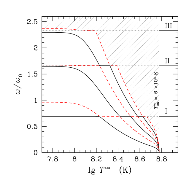
Fig. 3 shows the dependence of the pulsation eigenfrequencies $\omega$ on the red-shifted temperature $T^{\infty}\equiv T_{0}{\rm e}^{\nu_{0}/2}$ (we recall that the superfluid core is isothermal, in accordance with Eq. 31). The vertical dot-and-dashed line indicates the neutron critical temperature $T^{\infty}_{c{\rm n}}$. The horizontal dotted lines show the first three eigenfrequencies $\omega_{1}$, $\omega_{2}$, and $\omega_{3}$ for a non-superfluid star. No attempt to determine the spectrum in the shaded region was made. At $T^{\infty}>T^{\infty}_{c{\rm n}}$, the star pulsates as a normal fluid (no matter whether the protons are paired or not). Hence, the spectrum contains only normal, temperature-independent pulsation modes (the first three modes I, II, and III are shown as solid lines). At $T^{\infty}\;\raise 1.29167pt\hbox{$<$\kern-7.5pt\raise-4.73611pt\hbox{$\sim$}}\;0.1T^{\infty}_{c{\rm n}}$, a pulsating star can be described in the zero-temperature approximation. The spectrum of a cold superfluid star is doubled, as compared with that of a normal star (see Comer et al. 1999). In addition to “normal” pulsation modes, whose eigenfrequencies are close to those for a non-superfluid star (solid lines), the spectrum contains specific “superfluid” modes (dashed lines). Note that, the first “superfluid” mode is quite different from the “normal” one but the second and third “superfluid” modes are already sufficiently close to their “normal” counterparts (see Fig. 3).

As the temperature increases, starting from approximately $T^{\infty}\sim 10^{8}$ K, the frequency of each mode begins to decrease. When a mode reaches one of the horizontal dotted lines, it changes behavior and becomes temperature-independent, imitating the behavior of one of the non-superfluid modes. As the temperature rises further, the frequency of the higher mode approaches that of the mode in question, which in turn begins to decrease again (see avoiding crossings in Fig. 3). As a result, the two different modes of the spectrum will never intersect. One can conclude that a given mode may behave either as “superfluid” or “normal” with increasing temperature.

The behavior of the frequency spectrum at temperatures close to $T^{\infty}_{c{\rm n}}$ is of particular interest. It is clear from Fig. 3 that the frequency of any mode goes to zero at $T^{\infty}=T^{\infty}_{c{\rm n}}$. This is not surprising if we keep in mind that high order pulsation modes represent sound-like waves (see Section 5), and that the frequency of the “superfluid” sound also goes to zero at the transition point into the superfluid state (Fig. 1). It might seem that the spectrum does not contain eigenfrequencies of non-superfluid stars at the transition point when all neutrons in the star are normal. However, this is not the case. The point is that at $T^{\infty}\rightarrow T^{\infty}_{c{\rm n}}$, the number of modes with frequencies in any given interval, say, $[0,\omega_{1}]$, becomes infinitely large. As a result, at any temperature $T^{\infty}$ and any eigenfrequency of a normal star, there is a mode which is temporarily “normal-like”, i.e., it has the same frequency as in the normal fluid.

Since the temperature of neutron stars changes with time, it would be interesting to discuss how the pulsation frequencies vary with time. Suppose that the pulsation energy is much lower than the thermal energy. We can then neglect the star heating due to the conversion of pulsation energy into heat (see Gusakov et al. 2005 for details). The star will cool down, and to determine the dependence of the internal temperature $T^{\infty}$ on time $t$ one should use the cooling theory of superfluid neutron stars (see, e.g., Yakovlev et al. 1999, Yakovlev and Pethick 2004).

Since the direct Urca process is forbidden for the chosen neutron star model, the main cooling mechanisms (at $T^{\infty}<T^{\infty}_{c{\rm n}}$) will be neutrino emission due to Cooper pairing of neutrons, neutron-neutron bremsstrahlung, and the photon emission from the stellar surface. One can easily find the function $T^{\infty}(t)$ by solving the thermal balance equation (see, e.g., Yakovlev et al. 1999) under the assumption that the stellar core is isothermal. If the dependencies $\omega(T^{\infty})$ and $T^{\infty}(t)$ are known, it is possible to plot the frequency spectrum $\omega$ as a function of time $t$ (Fig. 4). Here the time (in units of $10^{3}$ years) is counted from the moment of neutron superfluidity onset (at $T^{\infty}=T^{\infty}_{c{\rm n}}$).

Figure 4: The dependence of the pulsation spectrum of a superfluid neutron star on time $t$, counted from the moment of neutron superfluidity onset (at $T^{\infty}=T^{\infty}_{c{\rm n}}$). The time is in units of $10^{3}$ years. Notations are the same as in Fig. 3.

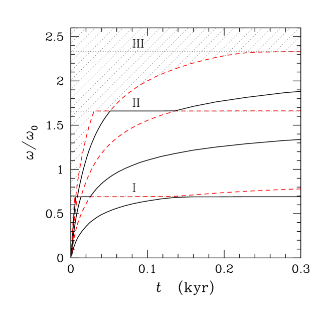
The analysis of Fig. 4 shows a significant change in the pulsation spectrum for 20 years after superfluidity turns on. This is associated with the highly efficient Cooper pairing neutrino emission (the detailed discussion of this process and its influence on the neutron star cooling is given by Gusakov et al. 2004). For example, the frequency of the third “superfluid” mode changes during this period of time from $0$ to the eigenfrequency $\omega_{2}$ of a non-superfluid star. The Cooper pairing neutrino emission process quickly becomes weaker with time, the cooling slows down and the variation in $\omega(t)$ becomes smoother. We would like to emphasize that the fast change of the pulsation frequencies for the first few dozens of years is due to the high critical temperature of neutrons, $T^{\infty}_{c{\rm n}}=6\times 10^{8}$ K. We could make the $\omega(t)$ dependence less dramatic by choosing lower critical temperatures.

7 Summary

The aim of the present study was to analyze radial pulsations of superfluid neutron stars at finite core temperatures. We used the equations for one-component superfluid hydrodynamics suggested by Son (2001), rewritten in terms of more convenient variables, and extended to the case of superfluid mixtures in General Relativity. A simple model of npe-matter was employed to show that a necessary condition for a star to be at hydrostatic and beta-equilibrium is constancy of the red-shifted temperature in the region of the star where the neutrons are superfluid: $T{\rm e}^{\nu_{0}/2}={\rm constant}$. Proton superfluidity does not impose any restrictions on the temperature, because protons are “coupled” with normal electrons by electromagnetic forces and behave as a normal fluid, no matter whether they are superfluid or not.

The hydrodynamics of superfluid mixtures was applied to investigate radial pulsations of neutron stars. It was assumed that the crust is non-superfluid, and neutrons and protons have red-shifted critical temperatures, which are constant throughout the core. The set of equations we have derived describes radial pulsations of superfluid stellar matter.

We have found the short wavelength solutions to this set of equations, representing sound waves in superfluid neutron star matter. The dependence of the speed of sound on the stellar temperature was examined in two limiting pulsation regimes: (1) in beta-equilibrated pulsating matter and (2) in pulsating matter with frozen nuclear composition. It was shown that three different kinds of sound waves may in principle exist, two of them propagate in the matter with frozen nuclear composition and one can exist only in beta-equilibrium. While the speeds of the former sound waves are comparable to each other (see Fig. 1) and to the speed of sound in the usual non-superfluid matter, the speed of the latter is 4–5 orders of magnitude lower (see Fig. 2); it can be excited only at temperatures $T$ close to $T_{c{\rm n}}$.

Generally, the pulsation equations were solved numerically, and the results show that the finite internal temperatures strongly affect the pulsation spectrum in the range of $T\sim(0.1-1)T_{c{\rm n}}$ (see Fig. 3). The frequency of any pulsation mode in this range decreases with increasing temperature. However, when the mode reaches one of the eigenfrequencies of a non-pulsating star, it becomes temperature independent for a while. One may say that it begins to mimic the behavior of a non-superfluid mode. At $T\rightarrow T_{c{\rm n}}$, all superfluid eigenfrequencies tend to zero. At $T\;\raise 1.29167pt\hbox{$<$\kern-7.5pt\raise-4.73611pt\hbox{$\sim$}}\;0.1T_{c{\rm n}}$, the pulsation spectrum is similar to that calculated in the zero temperature approximation.

In addition to the analysis of the temperature dependence of the pulsation spectrum, we discuss the temporal evolution of the eigenfrequencies during the star cooling (Fig. 4). In our analysis, we use the standard cooling theory of superfluid neutron stars (see, e.g., Yakovlev et al. 1999). The calculation shows that essential changes (within the present model) in the pulsation eigenfrequencies occur for the first 20 years following the moment of neutron superfluidity onset. This rather short (for the cooling theory) period of time is associated with the fast cooling due to the effective Cooper pairing neutrino emission process. It will be even shorter if the powerful direct Urca process operates in the stellar core.

The consideration of the problem presented here is based on a simplified model. In particular, we discuss only the simplest case of radial pulsations and assume critical temperatures of nucleons that are constant throughout the core. However, it would be important (and interesting) to understand how finite internal temperatures affect the frequency spectrum of non-radial pulsations and how the results would change if we analyzed more realistic density profiles for the critical temperatures. Finally, in a more realistic approach one should take into account ${}^{1}S_{0}$ neutron pairing in the stellar crust and more accurately treat the physics of the crust, especially if one deals with pulsation modes localized in the outer layers of the star. In spite of the considerable simplification of the problem discussed in this paper, we conclude that finite internal temperatures significantly affect the pulsation spectrum of not too cold superfluid neutron stars. Moreover, the pulsation frequencies can change dramatically for a period of several dozens of years, an effect that may potentially be observable.

References

- (1) Akmal A., Pandharipande V.R., 1997, Phys. Rev. C, 56, 2261
- (2) Alpar M.A., Langer Stephen A., Sauls J.A., 1984, ApJ, 282, 533
- (3) Andersson N., Comer G.L., 2001a, MNRAS, 328, 1129
- (4) Andersson N., Comer G.L., 2001b, Class. Quant. Grav., 18, 969
- (5) Andersson N., Comer G.L., Langlois D., 2002, Phys. Rev. D, 66, 104002
- (6) Andersson N., Comer G.L., Prix R., 2003, Phys. Rev. Lett., 90, 091101
- (7) Andreev A.F., Bashkin E.P., 1975, Zh. Eksp. Teor. Fiz., 69, 319 [1976, Sov. Phys. JETP, 42, 164]
- (8) Arkhipov R., Khalatnikov I., 1957, Zh. Eksp. Teor. Fiz., 33, 758
- (9) Borumand M., Joynt R., Kluniak W., 1996, Phys. Rev. C, 54, 2745
- (10) Carter B., in: Journes Relativistes 1976, edited by Cahen M., Debever R., Geheniau J. (Universit Libre de Bruxelles, Brussells, 1976), pp. 12–27
- (11) Carter B., in: Journes Relativistes 1979, edited by Moret-Baily I. and Latremolire C. (Facult des Sciences, Anger, 1979), pp. 166–182
- (12) Carter B., in: A Random Walk in Relativity and Cosmology, Proceedings of the Vadya-Raychaudhuri Festschrift, IAGRG, 1983, edited by Dadhich N., Krishna Rao J., Narlikar J.V., and Vishveshwara C.V. (Wiley Eastern, Bombay, 1985), pp. 48–62
- (13) Carter B., Khalatnikov I.M., 1992a, Phys. Rev. D, 45, 4536
- (14) Carter B., Khalatnikov I.M., 1992b, Ann. Phys., 219, 243
- (15) Carter B., Langlois D., 1998, Nucl. Phys. B, 531, 478
- (16) Chandrasekhar S., 1964, ApJ, 140, 417
- (17) Comer G.L., Langlois D., Lin L.M., 1999, Phys. Rev. D, 60, 104025
- (18) Comer G.L., Joynt R., 2003, Phys. Rev. D, 68, 023002
- (19) Gusakov M.E., Kaminker A.D., Yakovlev D.G., Gnedin O.Y., 2004, A&A, 423, 1063
- (20) Gusakov M.E., Haensel P., 2005, Nucl. Phys. A, 761, 333
- (21) Gusakov M.E., Yakovlev D.G., Gnedin O.Y., 2005, MNRAS, 361, 1415
- (22) Heiselberg H., Hjorth-Jensen M., 1999, ApJ, 525, L45
- (23) Haensel P., Levenfish K.P., Yakovlev D.G., 2000, A&A, 357, 1157
- (24) Haensel P., Levenfish K.P., Yakovlev D.G., 2001, A&A, 372, 130
- (25) Jackson A.D., Krotscheck E., Meltzer D.E., Smith R.A., 1982, Nucl. Phys. A, 386, 125
- (26) Khalatnikov I.M., 1952, Zh. Eksp. Teor. Fiz., 23, 169
- (27) Khalatnikov I.M., 1973, Pis’ma Zh. Eksp. Teor. Fiz., 17, 534
- (28) Khalatnikov I.M., Lebedev V.V., 1982, Phys. Lett. A, 91, 70
- (29) Khalatnikov I.M., 1989, An Introduction to the Theory of Superfluidity, Addison-Wesley, New York
- (30) Landau L.D., 1941, Zh. Eksp. Teor. Fiz., 11, 592
- (31) Landau L.D., 1947, J. Physics, 11, 91
- (32) Landau L.D., Lifshitz E.M., 1980, Statistical Mechanics, Part I, Course of Theoretical Physics, Pergamon Press, Oxford
- (33) Landau L.D., Lifshitz E.M., 1987, Fluid mechanics, Course of Theoretical Physics, Pergamon Press, Oxford
- (34) Langlois D., Sedrakian D.M., Carter B., 1998, MNRAS, 297, 1189
- (35) Lebedev V.V., Khalatnikov I.M., 1982, Zh. Eksp. Teor. Fiz., 83, 1623 [1982, Sov. Phys. JETP, 56, 923]
- (36) Lee U., 1995, A&A, 303, 515
- (37) Lindblom L., Mendell G., 1994, ApJ, 421, 689
- (38) Lombardo U., Schulze H.-J., 2001, in: Physics of Neutron Star Interiors, Springer Lecture Notes in Physics, Berlin, Eds. Blaschke D., Glendenning N.K., and Sedrakian A., v. 578, p. 30, astro-ph/0012209
- (39) Mastrano A., Melatos A., 2005, MNRAS, 361, 927
- (40) Mendell G., 1991a, ApJ, 380, 515
- (41) Mendell G., 1991b, ApJ, 380, 530
- (42) Negele J.W., Vautherin D., 1973, Nucl. Phys. A, 207, 298
- (43) Page D., Lattimer J.M., Prakash M., Steiner A.W., 2004, ApJS, 155, 623
- (44) Peralta C., Melatos A., Giacobello M., Ooi A., 2005, ApJ, 635, 1224
- (45) Prix R., Comer G.L., Andersson N., 2004, MNRAS, 348, 625
- (46) Pujol C., Davesne D., 2003, Phys. Rev. C, 67, 014901
- (47) Putterman S.J., 1974, Superfluid Hydrodynamics, North-Holland/American Elsevier, Amsterdam/New York
- (48) Reisenegger A., Jofr P., Fernndez R., Kantor E.M., ApJ, in press, astro-ph/0606322
- (49) Son D.T., 2001, Int. J. Mod. Phys., A16S1C, 1284
- (50) Tisza L., 1938, Nature, 141, 913
- (51) Villain L., Haensel P., 2005, A&A, 444, 539
- (52) Yakovlev D.G., Shalybkov D.A., 1991, A&SS, 176, 171
- (53) Yakovlev D.G., Levenfish K.P., Shibanov Yu.A., 1999, Physics-Uspekhi, 42, 737
- (54) Yakovlev D.G., Kaminker A.D., Gnedin O.Y., Haensel P., 2001, Phys. Rep., 354, 1
- (55) Yakovlev D.G., Pethick C.J., 2004, ARA&A, 42, 169
- (56) Yoshida S., Lee U., 2003, Phys. Rev. D, 67, 124019
- (57) Zhang S., 2003, Phys. Letters A, 307, 93