Likelihood Functions for Galaxy Cluster Surveys

Abstract

Galaxy cluster surveys offer great promise for measuring cosmological parameters, but survey analysis methods have not been widely studied. Using methods developed decades ago for galaxy clustering studies, it is shown that nearly exact likelihood functions can be written down for galaxy cluster surveys. The sparse sampling of the density field by galaxy clusters allows simplifications that are not possible for galaxy surveys. An application to counts in cells is explicitly tested using cluster catalogs from numerical simulations and it is found that the calculated probability distributions are very accurate at masses above several times $10^{14}h^{-1}M_{\odot}$ at $z=0$ and lower masses at higher redshift.

1. Introduction

The idea of using cluster surveys as probes of dark energy has generated considerable interest of late (Carlstrom et al., 2002; Haiman et al., 2001; Weller et al., 2001; Hu, 2003; Majumdar & Mohr, 2003; Lima & Hu, 2005). As the largest virialized objects in the universe, it is thought that clusters may be less affected by unknown or poorly understood astrophysical mechanisms and it is hoped that it will be reasonably straightforward to compare observed catalogs with theoretical estimates.

While many recent works have investigated the power of upcoming surveys and the challenges due to poorly understood selection effects, there has been relatively less attention in the literature to methods of analysis. It has been generally assumed that the problem can be separated into analyzing the differential number counts as a function of redshift and investigating the correlations (either angular or three-dimensional) in the cluster catalog. Studies of galaxy surveys have traditionally used either the power spectrum or $n$ point correlation functions to construct likelihood estimates, and most studies of the galaxy cluster abundance have assumed Poisson statistics. However, it has been recently emphasized that Poisson statistics for galaxy cluster surveys may not be a particularly good assumption (Hu & Kravtsov, 2003; Evrard et al., 2002).

The importance of sample variance considerations is two-fold. It broadens the probability distribution of the counts in cells, weakening constraints on the true number density, and the amount of this broadening is in principle directly calculable from theory, adding new information which in principle can be used to tighten constraints. As will be shown below, the effect of sample variance on cluster counts is not negligible and treating the counts as a Poisson process is incorrect.

In this work, we will go back to the work of White (1979) in galaxy clustering and update it to the context of galaxy cluster studies. In particular, we will derive the correct likelihood function to use for binned estimates of the cluster number counts and we write down an explicit expression for the likelihood of observing a particular galaxy cluster catalog as a function of theoretical models for the correlation structure of the density field. We will present some very preliminary tests using the catalogs from the Hubble volume simulation, demonstrating the regimes where these methods are robust and where more work clearly needs to be done.

2. Formalism

We adopt the formalism of Dodelson, Hui, & Jaffe (1997; hereafter DHJ97), which in turn closely follows the development of White (1979; hereafter W79). All that follows below is clearly outlined in W79 and the interested reader is referred to that paper for a full exposition.

The fundamental assumption is that the probability of observing an object at a particular location (in the absence of any other knowledge) is simply proportional to the number density of objects:

$$P(X_{1})=nw_{1}(\vec{x_{1}})dV_{1}$$ (1)

where $n$ is the number density, $w_{1}(\vec{x_{1}})$ is the survey weight at that point (the probability of detecting an object if it was at that point), and $dV_{1}$ is an infinitesimal volume around the position $\vec{x_{1}}$.

By similar reasoning, the probability of observing two objects at two points in space $\vec{x_{1}}$ and $\vec{x_{2}}$ can be expressed as

$$P(X_{1}X_{2})=n^{2}[w_{1}(\vec{x_{1}})w_{1}(\vec{x_{2}})+w_{2}(\vec{x_{1}},\vec{x_{2}})]dV_{1}dV_{2}$$ (2)

where $w_{2}(\vec{x_{1}},\vec{x_{2}})$ is the two-point correlation function, indicating the excess probability (over random) of detecting two objects at the given positions.

This reasoning can be extended to three objects:

$$P(X_{1}X_{2}X_{3}) = n^{3}\bigl{[}w_{1}(\vec{x_{1}})w_{1}(\vec{x_{2}})w_{1}(\vec{x_{3}})+$$

$$\sum w_{2}(\vec{x_{i}},\vec{x_{j}})w_{1}(\vec{x_{k}})+$$

$$w_{3}(\vec{x_{1}},\vec{x_{2}},\vec{x_{3}})\bigr{]}dV_{1}dV_{2}dV_{3}$$

with $w_{3}$ the three-point correlation function, and the sum refers to summing over all unique $i,j,k$. Obviously this can continue to even longer lists of objects.

A given catalog will contain $N$ objects, and the probability of detecting those $N$ objects at those positions can be constructed from the hierarchy of correlation functions, but a very useful component of the catalog is that there are no objects detected at other points. A quantity of interest is therefore the probability of detecting $N$ objects at observed $\vec{x_{i}}$ and no other objects at the other positions.

A recipe for incorporating this extra information was described in W79. Instead of using the functions $w_{i}$ that were used above, one can simply replace each occurrence of $w_{i}$ with $W_{i}$, where this latter quantity is simply

$$W_{i}(\vec{x_{1}},\vec{x_{2}},...,\vec{x_{i}})=\hskip 144.54pt$$ (4)

$$\sum_{j=0}^{\infty}{(-n)^{j}\over j!}\int...\int w_{i+j}(\vec{x_{1}},...\vec{x_{i+j}})dV_{i+1}...dV_{i+j}$$

It is nice to have an exact likelihood formulation for a given catalog, but a hierarchy of infinite sums can be a bit unwieldy. DHJ97 noted that for galaxy surveys there can easily be collections on the order of $10^{500}$ terms, even in the limit of Gaussianity and weak correlations. It will be shown below that galaxy cluster surveys the number of terms is quite manageable, at least in the limit of the cluster distribution being Gaussian and for a reasonably sparse survey. Cluster surveys can effectively be considered as perturbatively different from a Poisson distribution, allowing the probability distributions to be calculated quite efficiently.

In the Gaussian limit, it is useful to consider a few $W_{i}$:

$$W_{0}(V)=-nV+{n^{2}\over 2}\int dV_{1}dV_{2}w_{2}(\vec{x_{1}},\vec{x_{2}})$$ (5)

$$W_{1}(\vec{x_{1}})=1-n\int dV_{2}w_{2}(\vec{x_{1}},\vec{x_{2}})$$ (6)

$$W_{2}(\vec{x_{1}},\vec{x_{2}})=w_{2}(\vec{x_{1}},\vec{x_{2}})$$ (7)

where $V$ is the survey volume and the $w_{1}(\vec{x_{i}})$ have all been set to unity for simplicity. Note that this is not a requirement and is a straightforward way to include survey non-uniformity.

This allows an expression to be written down for observing a collection of points as a function of a theory which predicts the number density and two-point correlation function. To first order in the two-point function (DHJ97),

$$ln(P) = -nV+$$

$$\hskip-21.68121ptln\left[\prod_{a}W_{1}(\vec{x_{a}})+{1\over 2}\sum_{a}\sum_{b\neq a}{W_{2}(\vec{x}_{a},\vec{x}_{b})\over W_{1}(\vec{x}_{a})W_{1}(\vec{x}_{b})}\prod_{c}W_{1}(\vec{x}_{c})\right]$$

In the limit of sample variance being negligible (i.e., in the limit where $W_{i}$ approaches $w_{i}$), this approaches the likelihood one would expect for the number counts (the first term and the first term in brackets approaches the Poisson expression) combined independently with the correlation function. The second term in brackets closely resembles the likelihood one would obtain for the correlation function assuming that the probability of observing a pair at a given pair of locations is a Poisson process with mean given by $n^{2}(1+w_{2})$. When sample variance is not negligible, however, the probability will not be cleanly separable.

Furthermore, the same formalism was used by W79 to write down a compact expression for the counts-in-cells probability:

$$P[\Phi_{N}(V)]={(-nV)^{N}\over N!}{d^{N}\over dn^{n}}exp[W_{0}(V)]$$ (9)

where $\Phi_{N}(V)$ indicates observing $N$ objects (and only $N$) in a volume $V$.

Again, assuming weak correlations and working in the Gaussian limit, the counts in cells probability can be derived. Some details are derived in the appendix, but the result is straightforward. The probability of observing $N$ objects in a volume $V$ (to first order in the clustering) is

$$P[\Phi_{N}(V)]={x^{N}e^{-x}\over N!}\bigl{[}1-n^{2}V^{2}{\bar{w}\over 2}\bigl{(}{N-N^{2}\over x^{2}}+2{N\over x}-1\bigr{)}\bigr{]}$$ (10)

where $N$ is again the observed number, $x\equiv nV$, and $\bar{w}\equiv 1/V^{2}\int dV_{1}dV_{2}w_{2}(\vec{x_{1}},\vec{x_{2}})$ is the mean correlation function over the survey geometry. In calculations in this paper we use the second order expression to generate the figures, but a careful analysis of terms indicates that if the second order term is important then there is a good chance that all higher order terms must be included.

Where might this expression be expected to break down? In W79 it is clear that $W_{0}$ starts to become a challenging series when $nV\bar{w}$ becomes of order 0.1 or higher. We should therefore expect that this likelihood calculation will be most effective in that case and that it is suspect outside that regime. The breakdown appears to arise because the assumption of Gaussianity must always break down: the density field cannot be negative. With sparse sampling the probability of encountering a negative density is negligible and the assumption of Gaussianity is sufficient. However, at higher number densities the intrinsic non-Gaussianity becomes important.

Notice that this approach is straightforward to extend to objects that are tagged with an observable such as flux or richness. Going back to eqn 2, it should be sufficient to replace the initial number density with a sum over the individual number densities in each observable bin (e.g., theoretical number density as a function of optical richness or SZ flux), and then keep in mind that each $W_{i}$ will depend on the mass of the object or pairs of object under consideration. The efficacy of this technique is currently a topic of investigation.

3. Counts in Cells

We use the cluster catalogs derived from the Hubble volume simulations (Colberg et al., 2000) to test the range of validity of the likelihood expression derived for the counts in cells. A straightforward test is to use the $z=0$ cluster catalogs, where evolution effects can be neglected. We further specialize to the $\tau CDM$ simulation, where the transfer function is easy to reproduce. The simulation parameters are $\Omega_{m}=1.0,\sigma_{8}=0.6$ and $\Gamma=0.21$ and a box size of $2000h^{-1}Gpc$.

The volume is divided into subregions of cubic geometry and the above expressions are tested for a variety of cell sizes and mass thresholds. The number of clusters within each cell is then used to construct the probability distribution of the counts in cells. Mass thresholds were used to construct counts in cells for all objects above a threshold mass, with the mass defined as the number of particles (each of mass $2.2\times 10^{12}h^{-1}M_{\odot}$) found by the friends of friends algorithm with a linking parameter of 0.2.

The mean correlation function of the matter distribution was derived as

$$\bar{w} = {1\over V^{2}}\int dV_{1}dV_{2}w_{2}(\vec{x_{1}},\vec{x_{2}})$$

$$= {1\over 8\pi^{3}V^{2}}\int d^{3}kW(\vec{k})W^{*}(\vec{k})P(k)$$

where $W(\vec{k})$ is the window function for the cells (not related to the $W_{i}$ above!). For cubic cells, the window function is simply a product of $sinc$ functions.

The mean correlation function of the galaxy clusters needs to be corrected for the bias function. This is non-trivial; several fitting functions exist in the literature but typical errors appear to be on the order of 10% when applied in a regime where they have not been calibrated (Colberg et al., 2000). We use the bias relation of Sheth et al. (2001) with the mean bias for the cluster sample above a mass threshold derived using a mass function weighted bias factor. The mass function of Jenkins et al. (2001) was used, which has been calibrated using the simulation used here. In principle, given a mass correlation function one can estimate the bias as a function of an observable cluster property and use this to estimate the cluster mass as a function of cluster properties. However, current uncertainty in the theoretical understanding of bias as a function of mass in arbitrary cosmologies complicates any such undertaking.

An example is shown in figure 1. Taking a relatively high threshold of $6.6\times 10^{14}h^{-1}M_{\odot}$ and a cell size of 154 $h^{-1}$Mpc, the counts in cells distribution can be synthesized. We average over ten random cell offsets to smooth the observed distribution and compare it to the exact calculation of eqn 10. In the limit of massive (and therefore rare and sparse) clusters the likelihood for the counts in cells is quite accurate.

Figure 1.— Distribution of cell counts for clusters above $6.6\times 10^{14}H^{-1}M_{\odot}$ in Hubble Volume simulation compared to prediction from theory (broader distribution with lower peak) and corresponding result from same clusters with randomized positions (narrower distribution with higher peak).

The assumption of a Gaussian random field will break down when $nV\bar{w}$ is of order $10^{-1}$ (W79). To investigate the nature of the breakdown, we show in figure 2 the first breakdown for cells of size 100 Mpc and 133 Mpc. At higher masses (i.e., lower number densities) the theoretical result matches the simulations quite well. It is clear that there is noticeable deviation starting around $nV\bar{w}\gtrsim 0.5$. The mass thresholds were selected to straddle the transition. At yet lower masses, the theoretical result breaks down fairly comprehensively, developing bimodality. This is an indication that the theory is simply not well defined in this regime. It is impossible to set up a distribution of positive mass concentrations with vanishing correlation functions above the two-point function.

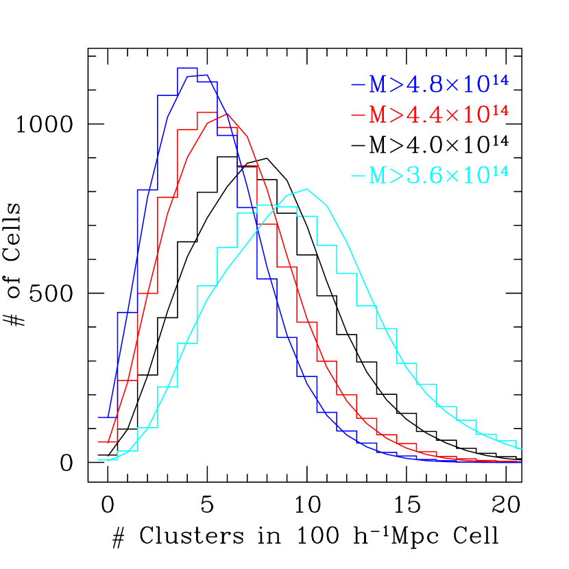
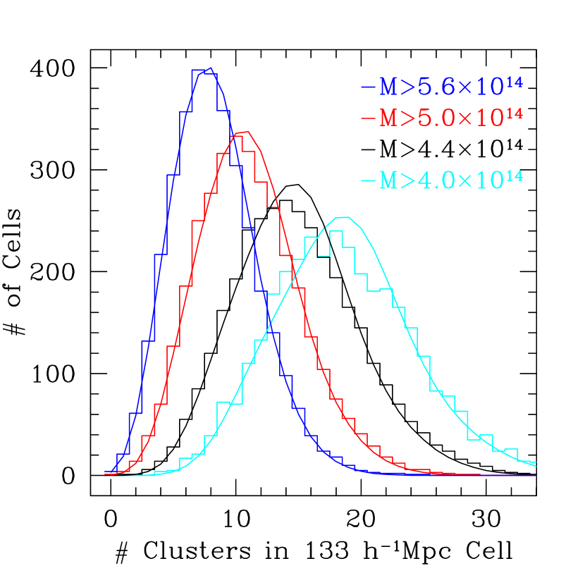
Figure 2.— Number of cells in simulation volume with given number of galaxy clusters above the mass threshold. The mass threshold is varied for two values of fixed cell size: 100 $h^{-1}$Mpc (left) and 133 $h^{-1}$Mpc (right). In the left panel, the values of $nV\bar{w}$ range from 0.44 to 0.68 (left to right in the figure) and in the right panel they range from 0.34 to 0.6

As the mass threshold is lowered, clusters become more numerous. As the cell size decreases, the mean number per cell will decrease but the mean correlation function over the cell volume will increase. For reasonable power spectra it turns out that the number per cell is slightly more important in this case for the purposes of calculating $nV\bar{w}$, making it slightly advantageous to move to smaller cell sizes.

To investigate the regime where this likelihood approach can be trusted, a grid of masses and cell sizes was investigated. The quantity $nV\bar{w}$ was calculated and the lines in figure 3 indicate the locus of pairs of $M$ and cell size that lead to $nV\bar{w}=0.5$. For a $\Lambda CDM$ model with $\sigma_{8}=0.9$ the likelihood approximation breaks down below $4\times 10^{14}h^{-1}M_{\odot}$, with the $\tau CDM$ breaking down around the same mass. However, this is a very steep function of the amplitude of the power spectrum. For example, using $\sigma_{8}=0.81$ drops the threshold of applicability to below $3\times 10^{14}h^{-1}M_{\odot}$. This is particularly relevant because this corresponds to the amplitude of fluctuations at $z=0.2$ if $\sigma_{8}=0.9$. Any survey for galaxy clusters at $z\gtrsim 0.2$ and targeting masses above a few $\times 10^{14}h^{-1}M_{\odot}$ is squarely is the regime where this likelihood calculation can be used.

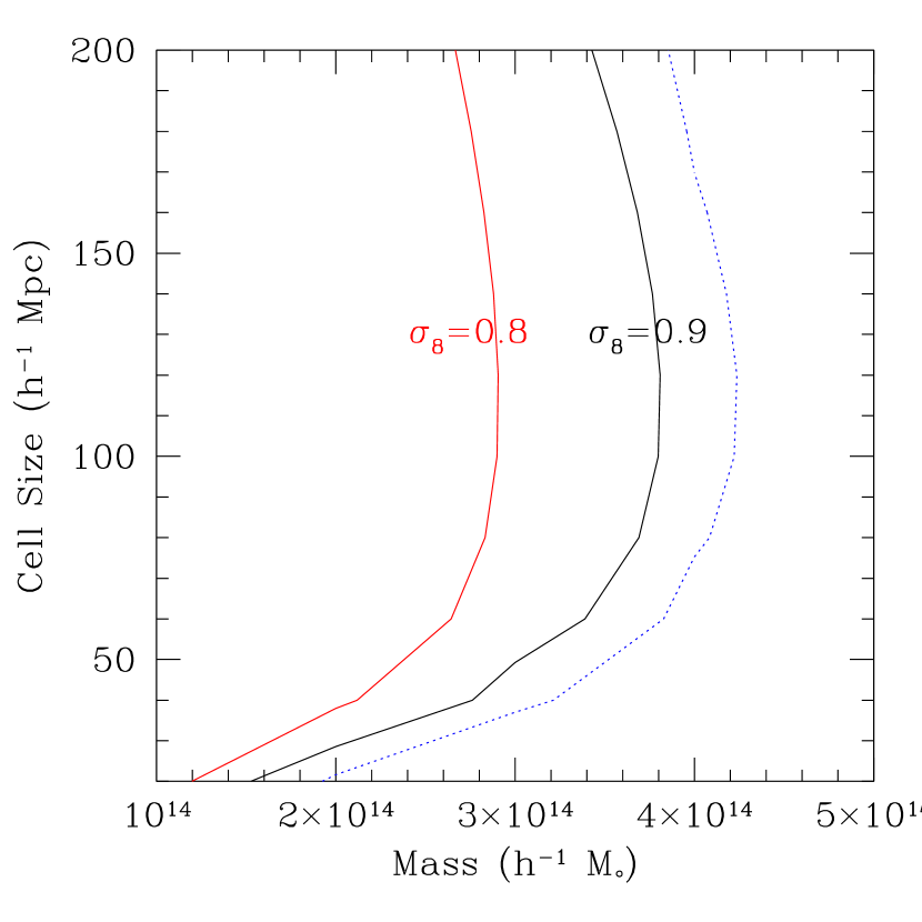
Figure 3.— Combinations of mass and cell size that lead to $nV\bar{w}=0.5$ assuming $\Omega_{M}=0.3,\Omega_{\Lambda}=0.7$, and power spectrum shape parameter $\Gamma=0.21$ for two values of $\sigma_{8}$. The dotted line corresponds to the $\tau CDM$ model that was used in the Hubble Volume simulations. The parameter space to the right of each line is in the regime of being easy to implement the likelihood formulation in this paper.

4. Outlook

The preliminary (and very highly idealized) tests outlined above demonstrate that many cluster surveys can be considered to be in the regime where catalog likelihood methods will be readily applicable. Tests on counts in cells at $z=0$ indicate that the non-Gaussianity of the cluster distribution becomes important around masses of several times $10^{14}h^{-1}M_{\odot}$. Applications of the cluster catalog likelihood (eqn 2) will likely have similar problems at lower masses and may also have difficulties at small separations. This is a topic of ongoing investigation.

The tests performed in this work used a $z=0$ simulation snapshot, rather than a lightcone selected volume. This was done to cleanly separate the possible complications and there is no conceptual problem with generalizing this to include redshift evolution. In fact, to generalize this one simply goes back to eqn 10 and allows $n,V,\bar{w}$ to be functions of $z$ and cosmological parameters, including the evolution of the relevant window functions. Non-cubic cell volumes that are functions of cosmological parameters and redshift will certainly complicate the analysis, but all the results presented here should be directly applicable.

There are several directions for more work in this area. Tests on existing cluster catalogs will yield insight into exactly how hard it is to implement these ideas in practice. One of the lessons learned is that this method works best on sparse catalogs (i.e., massive clusters), so in existing data it would be most easily tested on the most massive X-ray cluster surveys. It is unfortunate that the method appears to break down in a regime where there are high quality local cluster surveys.

On the theoretical side, an obvious next step is to apply these methods using clusters that have been additionally tagged with an observable such as X-ray or SZ flux or optical richness. Within this formalism such a modification is entirely straightforward, as all that is required are number densities and correlation strengths. Incorporating scatter in something like a mass-observable relation would be in principle straightforward, as would allowing for non-trivial (non power-law) evolution in such relations. However, uncertainty in the bias relations as a function of cosmology and mass must be improved to realize the full potential of these methods.

Given that the breakdown in this formalism appears to coincide with the onset of non-linearity, it may be possible to extend these results to lower masses with some modelling of the effects of weak non-linearity. The excellent match between theory and simulations at higher masses demonstrates that non-linearity and non-Gaussianity are not important in the high-mass regime.

5. Summary and Conclusions

In this paper we outlined a likelihood approach to galaxy cluster surveys that is uniquely applicable to the case of massive galaxy clusters. Essentially, for small enough sample and/or weak enough clustering strengths one can treat cluster catalogs as being expected to be drawn from a distribution that can be thought of as a Poisson distribution with some perturbations. By virtue of being only perturbatively different from a Poisson process, cluster catalogs lend themselves well to efficient likelihood estimation techniques that naturally include both shot noise and sample variance. This does not require an arbitrary conceptual breaking of the problem into “counts” and “clustering” but instead simply addresses the question of how likely it is to obtain a set of points given an assumed underlying correlation structure.

For galaxies, the number of terms involved in the estimate is prohibitive, and it is also important to understand the higher order correlations. That does not appear to be the case for massive galaxy clusters. The Gaussian weak correlation limit does a very good job of matching the counts in cells distribution for massive clusters in the Hubble volume simulation. As the mass threshold is lower, and the number density therefore increases, some disagreement arises, likely due to the number density becoming high enough that the distribution becomes sensitive to non-Gaussianity.

It should be emphasized that it is clearly not an advantage to have fewer clusters. One could always thin the number density of a sample until the catalog is in a regime where a catalog likelihood can be calculated. This would obviously be throwing away a huge amount of information and it seems unlikely that the gain in simplicity would be worth the loss of information.

These techniques are straightforward to generalize to explicitly include inhomogeneous survey selection and differential number densities and clustering strengths as a function of galaxy cluster properties.

With galaxy cluster surveys now being used for cosmological parameter estimation, it is essential to include the effects of sample variance to obtain accurate parameter estimates, so obtaining accurate probability distributions for counts in cells should be a high priority. The techniques here are a step in that direction, showing that such accurate distributions are easily calculated for massive galaxy clusters.

As this article neared completion, an article appeared by Hu & Cohn discussing very similar ideas from a slightly different perspective. The results here largely agree with theirs in the aspects where they overlap.

Appendix A Details of the Counts in Cells Likelihood

The calculation of the likelihood for counts in cells can be derived from equation 9 with straightforward algebra and accounting in the limit of weak clustering. Some of the details are spelled out below.

$$P[\Phi_{N}(V)]={(-nV)^{N}\over N!}{d^{N}\over dn^{n}}exp[W_{0}(V)]$$ (A1)

Define $x\equiv nV$ and using $W_{0}=-x+x^{2}\bar{w_{2}}/2$, the first step is to expand the exponential term as a Taylor series. For convenience, define $\alpha\equiv\bar{w_{2}}/2$ and the counts in cells probability distribution can be written

$$P[\Phi_{N}(V)]={(-x)^{N}\over N!}{d^{N}\over dx^{N}}\left(\sum_{i=0}^{\infty}{1\over i!}(-x)^{i}[1-\alpha x]^{i}\right)$$ (A2)

Expanding the part inside the sum with the binomial expansion gives

$$P[\Phi_{N}(V)]={(-x)^{N}\over N!}{d^{N}\over dx^{N}}\left(\sum_{i=0}^{\infty}\sum_{k=0}^{i}{1\over k!(i-k)!}(-x)^{i+k}\alpha^{k}\right)$$ (A3)

The effect of the derivatives is that all terms in the sums with $i+k<N$ are set to zero and all other terms are multiplied by $x^{-N}(i+k)!/(i+k-N)!$:

$$P[\Phi_{N}(V)]={(-x)^{N}\over N!}\left(\sum_{i=0}^{\infty}\sum_{k=max(0,N-i)}^{i}(-1)^{N}{(i+k)!\over k!(i-k)!(i+k-N)!}\alpha^{k}(-x)^{i+k-N}\right)$$ (A4)

Up to this point, the only assumption implicit in this analysis is that the correlation functions beyond the two-point function are negligible. To see the structure in the probability distribution, we now assume that $\alpha$ is small and investigate the relevant terms in the above equation. In particular, for small $\alpha$ the only important terms will be terms with small $k$. This immediately identifies the important terms as being the ones with $i$ close to $N$.

For the terms with $k=0$, we are left with the sum

$$k=0:\ \ \sum_{i=N}^{\infty}{1\over(i-N)!}(-x)^{i-N}=e^{-x}$$ (A5)

which reproduces the Poisson probability in the case of zero correlations.

To first order in $\alpha$, one can move to one lower value of $i$:

$$k=1:\ \ \alpha\sum_{i=N-1}^{\infty}{(i+1)!\over(i+1-N)!(i-1)!}(-x)^{i+1-N}=-\alpha e^{-x}(N^{2}-N-2xN+x^{2})$$ (A6)

and to second order in $\alpha$ we can continue down:

$$k=2:\ \ \alpha^{2}\sum_{i=N-2}^{\infty}{(i+2)!\over 2(i+2-N)!(i-2)!}(-x)^{i+2-N} = {\alpha^{2}\over 2}e^{-x}(-8xN+12xN^{2}+6x^{2}N^{2}-6x^{2}N-$$ (A7)

$$4x^{3}N+11N^{2}-6N^{3}-6N-4xN^{3}+x^{4}+N^{4})$$

with subsequent orders obtained similarly. These sums are straightforward to implement using software such as Maple but can become tedious. In all that was implemented in this work the series was truncated at second order.

The sums have an interesting property that each term seems to be of order $(\alpha x^{2})^{k}$, since $N$ is of the same order as $x$. At each level the terms are actually of lower order in $x$ due to cancellations in the sums. For example, for $x=N$ the expression in brackets in equation A7 reduces to $3N^{2}-6N$, making this term roughly $\alpha^{2}x^{2}$. Nonetheless, it is clear that simply having small $\alpha$ is not sufficient. For this formalism to be useful it is required that $\alpha x$ be small, at least, and it is preferable that $\alpha x^{2}$ be small to be sure that all higher order terms are negligible. It is apparent from the expression for $W_{0}$ that bad things are happening as $\alpha x$ is becoming large, since it is becoming dubious that the void probability function is bounded to be less than one (i.e., $W_{0}$ must be negative). This is likely a breakdown of the physical picture of Poisson sampling of a Gaussian random field, rather than a breakdown of any approximations. It is impossible to Poisson sample with a negative mean, which a Gaussian random field allows. The requirement that the density is non-negative necessitates some amount of non-Gaussianity. With enough samples, this non-Gaussianity must manifest itself in the observed distribution.

References

- Carlstrom et al. (2002) Carlstrom, J. E., , Holder, G. P., & Reese, E. D. 2002, ARA&A, 40, 643
- Colberg et al. (2000) Colberg, J. M., White, S. D. M., MacFarland, T. J., Jenkins, A., Pearce, F. R., Frenk, C. S., Thomas, P. A., & Couchman, H. M. P. 2000, MNRAS, 313, 229
- Dodelson et al. (1997) Dodelson, S., Hui, L., & Jaffe, A. 1997, ArXiv Astrophysics e-prints
- Evrard et al. (2002) Evrard, A. E., MacFarland, T. J., Couchman, H. M. P., Colberg, J. M., Yoshida, N., White, S. D. M., Jenkins, A., Frenk, C. S., Pearce, F. R., Peacock, J. A., & Thomas, P. A. 2002, ApJ, 573, 7
- Haiman et al. (2001) Haiman, Z., Mohr, J. J., & Holder, G. P. 2001, ApJ, 553, 545
- Hu (2003) Hu, W. 2003, Phys. Rev. D, 67, 081304
- Hu & Cohn (2006) Hu, W., & Cohn, J. D. 2006, ArXiv Astrophysics e-prints
- Hu & Kravtsov (2003) Hu, W., & Kravtsov, A. V. 2003, ApJ, 584, 702
- Jenkins et al. (2001) Jenkins, A., Frenk, C. S., White, S. D. M., Colberg, J. M., Cole, S., Evrard, A. E., Couchman, H. M. P., & Yoshida, N. 2001, MNRAS, 321, 372
- Lima & Hu (2005) Lima, M., & Hu, W. 2005, Phys. Rev. D, 72, 043006
- Majumdar & Mohr (2003) Majumdar, S., & Mohr, J. J. 2003, ApJ, 585, 603
- Sheth et al. (2001) Sheth, R. K., Mo, H. J., & Tormen, G. 2001, MNRAS, 323, 1
- Weller et al. (2001) Weller, J., Battye, R., & Kneissl, R. 2001, Phys. Rev. Lett., 88, 231301
- White (1979) White, S. D. M. 1979, MNRAS, 186, 145