The ESO-Spitzer Imaging extragalactic Survey (ESIS) I:
WFI B,V,R deep observations of ELAIS-S1 and comparison to Spitzer and GALEX data

Abstract

Context. The ESO-Spitzer extragalactic Imaging Survey (ESIS) is the optical follow up of the Spitzer Wide-Area InfraRed Extragalactic (SWIRE) survey in the ELAIS-S1 area.

Aims. The multiwavelength study of galaxy emission is the key to understand the interplay of the various components of galaxies and to trace their role in cosmic evolution. ESIS provides optical identification and colors of Spitzer IR galaxies and builds the bases for photometric redshift estimates.

Methods. This paper presents B, V, R Wide Field Imager observations of the first 1.5 square degree of the ESIS survey. Data reduction is described including astrometric calibration, illumination and color corrections. Synthetic sources are simulated in scientific and super-sky-flat images, with the purpose of estimating completeness and photometric accuracy for the survey. Number counts and color distributions are compared to literature observational and theoretical data, including non-evolutionary, PLE, evolutionary and semi-analytic $\Lambda$CDM galaxy models, as well as Milky Way stellar predictions. The ELAIS-S1 area benefits from extensive follow-up from X-ray to radio frequencies: some potential uses of the multi-wavelength observations are illustrated.

Results. Object coordinates are defined with an accuracy as good as $\sim 0.15$ $[$arcsec$]$ r.m.s. with respect to GSC 2.2; flux uncertainties are $\sim$2, 10, 20% at mag. 20, 23, 24 respectively (Vega); we reach 95% completeness at B,V$\sim$25 and R$\sim$24.5. ESIS galaxy number counts are in good agreement with previous works and are best reproduced by evolutionary and hierarchical $\Lambda$CDM scenarios. Optical-Spitzer color-color plots promise to be very powerful tools to disentangle different classes of sources (e.g. AGNs, starbursts, quiescent galaxies). Ultraviolet GALEX data are matched to optical and Spitzer samples, leading to a discussion of galaxy properties in the UV-to-24 $\mu$m color space. The spectral energy distribution of a few objects, from the X-rays to the far-IR are presented as examples of the multi-wavelength study of galaxy emission components in different spectral domains.

1 Introduction

The assembly and evolution of galaxies, galaxy clusters and cosmic large-scale structure (LSS) are currently major issues in both theoretical and observational cosmology. Tracing the history of cosmic star formation and the growth of the cosmic stellar mass density will lead to an understanding of the fundamental processes transforming the primordial diffuse plasma into the highly structured present-day Universe.

The multi-wavelength study of the emission of galaxies provides tools to disentangle their different physical components. Young stellar populations power the UV-optical light, old stars emit predominantly in the near-IR, while dust — heated by either starburst activity or an active galactic nucleus (AGN) — dominates the mid- and far-IR luminosity. X-ray and radio luminosities are also produced by starbursts or AGNs. Extending the analysis of galaxy properties to as wide a redshift range as possible is compulsory, in order to understand the interplay of the various components and to trace their role in cosmic galaxy evolution.

The two main instruments onboard Spitzer, observing in the mid- to far-IR ($3-8\ \mu$m for IRAC and 24, 70, 160 $\mu$m for MIPS), were specifically designed to probe the old stellar content and dust re-radiation from distant galaxies.

The cosmic Infra-Red Background (CIRB, Puget et al. 1996; Hauser et al. 1998), discovered by the COBE satellite in the mid 90’s, is the most energetic diffuse radiation after the CMB. Elbaz et al. (2002) and Franceschini et al. (2003) have shown that at least 50% of the CIRB emission is powered by luminous and ultra-luminous massive star-forming galaxies, at redshift $z=0.5-1.5$, strongly evolving in cosmic time. The Universe seems to have experienced a phase of enhanced activity of star-formation and gravitational accretion in the past, mostly visible in the infrared (e.g. Franceschini et al. 2001).

The Spitzer Multiband Imaging Photometer (MIPS, Rieke et al. 2004) provides the observations needed to push the study of mid- and far-IR sources to fainter luminosities and larger distances. Polycyclic Aromatic Hydrocarbon (PAH) emission, typical of starburst 7-13 $\mu$m restframe spectra, is sampled by MIPS up to redshift $\sim 3$, corresponding to an epoch when the Universe had only $\sim$15% of today’s age.

A central issue in modern cosmology is when galaxies assembled their baryonic mass. The hierarchical scenario (e.g. Kauffmann & Charlot 1998) predicts that the most massive systems (e.g. $M_{\textrm{stars}}>10^{11}$ M_⊙) formed relatively late through a slow process of merging of smaller galaxies. In monolithic-collapse models (Eggen et al. 1962), the bulk of stars formed in early-type galaxies at very high redshift, while subsequent merging and star formation are limited. Modern $\Lambda$CDM models and hydrodynamical simulations (e.g. Nagamine 2001) implement a mixture of the two.

Several studies have attempted to investigate the formation and evolution of massive systems and test model predictions (see, e.g., the recent works by Drory et al. 2005; Treu 2004; Fontana et al. 2004; Cimatti 2003), but a clear and coherent picture has not yet emerged. Very little is known about galaxy stellar mass assembly at redshift $z>1.5$ (e.g. Cimatti 2003; Daddi et al. 2004).

The Infrared Array Camera (IRAC, Fazio et al. 2004) onboard Spitzer observes in the $3.6-8.0$ $\mu$m wavelength range. The instrument was specifically designed for detecting galaxies’ restframe near-IR emission, up to redshift $z\geq 3$, hence directly probing their stellar mass assembly.

1.1 The SWIRE & ESIS Surveys

A significant fraction of the first year of Spitzer in-flight operations has been devoted to six different Legacy science Programs, representing projects of general and lasting importance to the broad astronomical community. Among these, SWIRE (Lonsdale et al. 2003, 2004) and GOODS (Dickinson et al. 2003) are dedicated to cosmology.

The Spitzer Wide-area Infra-Red Extragalactic survey (SWIRE) is the largest Spitzer Legacy Program. It consists of a wide-area, imaging campaign designed to trace the evolution of dusty, star-forming galaxies, evolved stellar populations, and AGN as a function of environment, from redshifts $z\sim 3$, down to the current epoch. SWIRE includes 6 high-latitude fields, totaling 49 $[$deg${}^{2}]$ in all the seven Spitzer bands.

The large sky area covered by the SWIRE survey implies large galaxy samples of all kinds, secures high statistical significance to clustering and galaxy evolution studies, and allows the possibility of rare object searches.

The ESO-Spitzer wide-area Imaging Survey (ESIS) is an ESO Large Programme (P.I. Alberto Franceschini), securing optical ground-based imaging follow-up to the SWIRE Spitzer survey in the ELAIS-S1 field.

The ELAIS-S1 region, together with Lockman Hole, is the highest priority region for SWIRE, thanks to the extremely low 100 $\mu$m cirrus emission (Schlegel et al. 1998). In fact, it includes the absolute minimum of the Galactic 100 $\mu$m emission in the Southern sky.

A broad wavelength coverage is required by the nature of the sources we are targeting, which are typically reddened, and/or with old evolved stellar populations, and at high redshifts. These properties imply dramatic difficulties when trying to acquire spectroscopic follow-up in the optical. Photometric investigation of the properties of faint sources provides a very powerful alternative, and it is clearly the only viable approach when dealing with large datasets over wide areas.

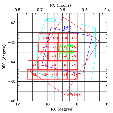
Figure 1: ESIS WFI (BVR) pointings scheduled in the ELAIS S1 region: a total of 22 fields (red numbered small squares) of $30^{\prime}\times 30^{\prime}$ are being observed as part of the ESIS survey. The region observed by ISO (Oliver et al. 2000), the Spitzer/SWIRE field (Lonsdale et al. 2003) and the ATCA radio survey by Gruppioni et al. (1999) are marked. The four circles represent XMM observations. Regions 3-6 have also been observed with SOFI/NTT with J and Ks filters, during Summer 2002. See Section 6 for a review of the available data in ELAIS-S1.

ESIS covers $\sim 5$ $[$deg${}^{2}]$ in 5 optical bands and is based on imaging with the Wide Field Imager (WFI, at the focal plane of the 2.2m La Silla ESO-MPI telescope, Baade et al. 1999) and the VIsible Multi Object Spectrograph (VIMOS, on VLT, Le Fèvre et al. 2002; D’Odorico et al. 2003) to $\sim 25-26$ mag in BVRIz. The total amount of scheduled observing time is 27 nights with the WFI and 8 nights with VIMOS.

Prime motivations for ESIS are to:

• obtain optical identification for the roughly 300000 IR sources detected by SWIRE in the 5 $[$deg${}^{2}]$ of the ESIS area; the present statistics on Spitzer sources indicate that $\sim 80$% of the SWIRE IRAC sources could be detected to $B=26$ and $V=25.5$;

• provide colors and rough morphologies for source classification;

• build the basis for photometric redshifts for all IR sources, and optimize the spectroscopic IR and optical follow-up;

• provide UV-blue restframe luminosities of IR galaxies;

• produce independent optical samples, selected on the basis of their restframe UV-blue properties, for comparison with the IR-selected ones.

This paper describes WFI observations, data reduction and analysis in the central ELAIS-S1 1.5 $[$deg${}^{2}]$. VIMOS observations will be characterized in a forthcoming paper and subsequent releases of WFI data will be presented on the ESIS official web page. The data described here are being included in the third SWIRE Spitzer Legacy data release (Fall 2005).

Section 2 deals with optical Wide Field Imager service mode observations. Data reduction is described in Section 3, where astrometric accuracy, catalog extraction and photometric calibration are also discussed. In Section 4, we present a set of simulations carried out with the purpose of estimating the effective depth of the survey and flux uncertainties. Section 5 deals with source number counts, disentangling point-like and extended objects and comparing ESIS to literature data and predictions of galaxy evolutionary models. In Section 6, the ESIS catalog is matched to multiwavelength data in the ELAIS-S1 area, spanning from the X-rays to the far-infrared, illustrating the potential of panchromatic studies of galaxies. Finally, in Section 7, we summarize current findings.

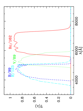
Figure 2: Transmission curves for ESIS WFI observations.

Exp. #	$\Delta\alpha$	$\Delta\delta$
1	0	0
2	+32	+24
3	–32	+48
4	–48	–24
5	+48	–48

Table 1: Dithering pattern in $[$arcsec$]$ of WFI BVR observations. Each pointing consists of 30 dithered exposures (6 sets of 5). The shifts reported here refer to the first exposure of each set.

Field			B band			V band			R band
Exposure	$\alpha$	$\delta$	Date	Airmass	Seeing	Date	Airmass	Seeing	Date	Airmass	Seeing
set	$[$hh:mm:ss$]$	$[^{\circ}:^{\prime}:^{\prime\prime}]$	dd/mm/yy	(avg)	$[^{\prime\prime}]$	dd/mm/yy	(avg)	$[^{\prime\prime}]$	dd/mm/yy	(avg)	$[^{\prime\prime}]$
1_1	00:38:30.0	-43:43:00	10/10/01	1.338	0.81	10/10/01	1.502	0.83	10/10/01	1.222	0.71
1_2			11/10/01	1.313	0.86	24/10/01	1.034	1.07	24/10/01	1.210	0.92
1_3			11/10/01	1.153	0.70	17/11/01	1.048	1.05	24/10/01	1.131	0.98
1_4			12/10/01	1.281	1.09	17/11/01	1.034	0.83	24/10/01	1.080	0.88
1_5			12/10/01	1.182	1.10	17/11/01	1.035	0.84	22/10/01	1.049	0.82
1_6			13/10/01	1.283	1.08	14/12/01	1.133	0.89	24/10/01	1.083	1.06
2_1	00:38:26.4	-43:15:00	06/11/01	1.063	0.98	06/11/01	1.048	1.03	06/11/01	1.143	0.97
2_2			24/10/01	1.174	1.02	24/10/01	1.084	1.10	24/10/01	1.048	1.08
2_3			09/07/02	1.040	0.82	08/07/02	1.038	0.91	10/08/02	1.042	0.80
2_4			09/07/02	1.030	0.88	10/07/02	1.032	1.00	14/08/02	1.126	0.87
2_5			11/07/02	1.148	1.05	11/07/02	1.053	0.95	14/08/02	1.043	0.72
2_6			11/07/02	1.229	1.09	11/07/02	1.090	0.96	14/08/02	1.149	0.71
3_1	00:35:52.0	-43:15:00	11/10/01	1.479	0.91	11/10/01	1.503	1.01	22/10/01	1.170	0.72
3_2			06/11/01	1.032	1.02	06/11/01	1.086	1.02	06/11/01	1.236	1.07
3_3			13/10/01	1.147	1.04	30/09/02	1.042	1.06	30/09/02	1.061	0.78
3_4			20/10/03	1.108	0.91	30/09/02	1.031	1.00	18/11/01	1.031	1.05
3_5			10/10/01	1.277	0.80	30/09/02	1.036	0.83	30/09/02	1.104	0.93
3_6			09/10/01	1.271	0.97	30/10/03	1.050	0.90	20/10/03	1.035	0.71
4_1	00:35:54.4	-43:43:00	28/11/03	1.038	0.99	28/10/02	1.064	1.18	28/10/02	1.109	1.04
4_2			28/11/03	1.182	1.00	11/07/02	1.035	1.13	20/10/03	1.149	0.72
4_3			30/10/03	1.102	0.73	11/07/02	1.034	1.03	30/10/03	1.138	0.75
4_4			01/11/03	1.036	0.98	20/10/03	1.089	0.77	30/10/03	1.219	0.92
4_5			30/10/03	1.129	0.94	30/10/03	1.066	0.75	01/11/03	1.075	0.89
4_6			20/10/03	1.040	0.94	12/07/02	1.122	1.10	30/10/03	1.033	0.98
5_1	00:33:17.6	-43:15:00	27/10/02	1.071	1.02	27/10/02	1.120	0.97	27/10/02	1.193	1.02
5_2			30/11/03	1.140	0.77	30/11/03	1.047	0.83	30/11/03	1.082	0.90
5_3			28/11/03	1.388	1.04	28/11/03	1.255	0.95	30/11/03	1.226	0.76
5_4			05/01/05	1.535	0.91	30/11/03	1.418	0.85	10/01/05	1.521	0.94
5_5
5_6			20/10/03	1.141	0.70	20/10/03	1.233	0.80	20/10/03	1.383	0.72
6_1	00:33:18.8	-43:43:00				30/10/02	1.065	1.25
6_2			30/10/02	1.040	1.22				30/10/02	1.110	1.30
6_3
6_4
6_5
6_6			21/10/03	1.086	0.70	21/10/03	1.222	0.70	21/10/03	1.141	0.78

Table 2: Summary of WFI, BVR observations. Each set of exposures consists of five 300 $[$s$]$ frames. Observing dates and average airmasses are reported for each set. Seeing values have been measured directly on science frames.

2 Observations

The ESIS WFI survey consists of BVR imaging observations of ELAIS-S1, carried out in Service mode between October 2001 and January 2005. Further observations are scheduled and will be continued until completion of the entire 5 $[$deg${}^{2}]$ planned area.

The ESIS field has been divided into 22 different sub-areas, each corresponding to one WFI $30^{\prime}\times 30^{\prime}$ pointing. The different pointings overlap by about 1.5^′ on each side to obtain a full coverage and to allow trimming individual images to avoid edge effects.

Figure 1 shows the WFI coverage of the ELAIS-S1 ESIS sky area, as well as the SWIRE, ISO, XMM, ATCA fields. The SWIRE and ESIS fields are shifted relative to one another because of resizing of the original Spitzer area. Section 6 will describe the available multi-wavelength observations in ELAIS-S1.

The WFI array is made of 8 CCDs, separated by small gaps. In order to fill these gaps and correct bad pixels and cosmic ray events, each $30^{\prime}\times 30^{\prime}$ field is covered by 6 sets (Observing Blocks, OBs) of 5 dithered exposures. At least one of the six OBs per pointing per band was observed during a photometric night, as required by the scheduling. The standard WFI dithering pattern (see Tab. 1) was used. The scale of the instrument is 0.238 $[$arcsec/pixel$]$.

Each single exposure consists of 300 $[$s$]$, for a total exposure time of 2.5 hours per pointing per band (B, V, R).

The filters used are WFI B/99, V/89 and Rc/162. Observing Blocks defined after September 2002 (i.e. starting from pointing no. 5) have B/123 instead of B/99, because the standard WFI filters and calibration plan changed; in this paper we refer to B,V,R, regardless of which are involved. There are no significant differences in the final catalog, which is calibrated to the Johnson-Cousins system (see Sect. 3.4). Figure 2 shows the transmission functions for the 4 filters.

Table 2 summarizes the observing logs for the central 6 fields (i.e. 1.5 $[$deg${}^{2}]$). Field 6 observations have not been completed yet, but this field is included in this paper because it covers part of the area observed in the X-rays and near-IR. The seeing and airmass values are the averages on the 5 images constituting each OB. The majority of nights satisfied the requested observing constraints: seeing$<$1.2″, moon distance $>$120^∘, moon phase $<0.4$. Aborted, or out-of-requirements OBs are not listed in Table 2, apart from those for pointing no. 6.

3 Data Reduction

The reduction of ESIS data was performed within the IRAF environment, using the package WFPRED developed by two of us (LR, EVH) at the Padova Astronomical Observatory. This package consists of a set of procedures that access and upgrade the standard MSCRED (Valdes 1998) tasks.

Correction of bias and flat-fielding followed the standard procedure. Sky flat-field frames were acquired during each night and applied to images obtained on the same date.

3.1 Super-Sky-Flat Field

Even if sky flat-field frames were used, significant illumination gradients exist on the pre-reduced frames. Hence a further correction was needed, both to obtain a uniform background and to build frames with the same photometric zeropoint across the whole field of view. The main causes for these gradients are:

1. sky flat fields point at different positions on the sky than the science target, and therefore have different relative positions to the moon and very bright stars;

2. bright off-axis sources produce spurious multiple reflections in the focal reducer of WFI;

3. the moon, when present, produces smooth gradients in the background of science frames.

To address these issues, Super-sky-flat field frames (hereafter ss-flat) were produced, by combining all science frames obtained during a given night. The adopted procedure is sketched below.

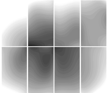
Figure 3: Example of R-band super-sky-flat frame (negative rendered).

• In order to create the ss-flat, astronomical objects must be removed from the science images. Detection of all sources and build up of object masks were performed with the objmasks task in the MSCRED IRAF package.

• Very bright sources (e.g. luminous stars and big galaxies) produce very extended halos on the images. All science frames were visually inspected and all halos were manually masked.

• All science frames were then combined together, using object-masks to cancel-out the light coming from astronomical sources.

• The result was fitted with a 2-dimensional 4th order Legendre function, obtaining a smoothed, but accurate representation of the ss-flat. Alternatively, a simple boxcar smoothing was also tested, but it was found that Legendre fitting led to better results, because it avoids “holes” produced by the large masks on extended halos.

An example of R band ss-flat is shown in Figure 3.

Since the targeted fields lie all roughly at the same equatorial coordinates, the same ss-flat was applied to all the images taken during a given night, unless significant changes in sky conditions (e.g. presence of atmospheric cirrus) occurred.

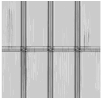
Figure 4: Weight mask for R-band ESIS WFI pointing no. 2, used during the detection of sources and the estimation of photometric uncertainties.

3.2 Astrometric calibration and co-addition

Reduction of wide field imaging data requires a detailed astrometric calibration, in order to take into account the intrinsic distortions of the instrumentation, and minimize the effect of projecting a large sky area (intrinsically spherical) onto a planar CCD.

In the case of WFI ESIS data, the $30^{\prime}\times 30^{\prime}$ field of view requires particular care when mapping pixels into celestial coordinates. In view of multi-wavelength cross-correlation and future spectroscopic follow up in the ELAIS-S1 area, as good an astrometric calibration as possible is necessary.

An accurate solution is provided by the TNX transformation, that combines a linear projection of the sky sphere onto a tangent plane (the standard gnomonic algorithm, TAN, Calabretta & Greisen 2002) and a polynomial function for distortions. A simplified description of the adopted mapping is:

$$\left(\begin{array}[]{c}\xi^{\prime}\\ \eta^{\prime}\end{array}\right) = \left(\begin{array}[]{c}\xi\\ \eta\end{array}\right)+\left(\begin{array}[]{c}lngcor[\xi,\eta]\\ latcor[\xi,\eta]\end{array}\right)$$ (7)

$$\left(\begin{array}[]{c}\xi\\ \eta\end{array}\right) = \left(\begin{array}[]{cc}a_{11}&a_{12}\\ a_{21}&a_{22}\end{array}\right)\left(\begin{array}[]{c}x-x_{c}\\ y-y_{c}\end{array}\right)$$ (14)

where $(\xi^{\prime},\eta^{\prime})$ are the celestial coordinates on the sky, mapped by the TNX algorithm, $(\xi,\eta)$ represent the first-order solution of the TAN transformation (given by the $a$ matrix), $(x,y)$ and $(x_{c},y_{c})$ are the cartesian coordinates of the generic pixel and of the image center, $lngcor$ and $latcor$ are the polynomial equations mapping distortions along longitude and latitude.

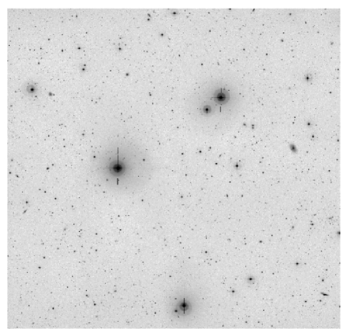
Figure 5: Final, co-added, R-band frame of ESIS WFI Field number 3.

The solution of the above equation array is built on dedicated observations of Stone et al. (1999) astrometric fields D and E, carried out as part of the ESIS program. Since observations are spread along a wide period of time, several different astrometric solutions have been necessarily built, because extra-ordinary maintenance of the WFI camera affected the pixels$\rightarrow$celestial coordinates map.

The best results were obtained using 4th order distortion polynomials. Every individual image was astrometrically calibrated before co-addition. After the solution was applied, frames were finely re-centered by means of rigid shifts to the GSC 2.2 (STScI & OaTO, 2001) catalog.

During co-addition, all frames were re-projected, transforming their astrometric map to a common one (that for the B band), regardless of the photometric band. This choice allows the B, V, and R images to be easily compared and 3-band catalogs to be straightforwardly produced.

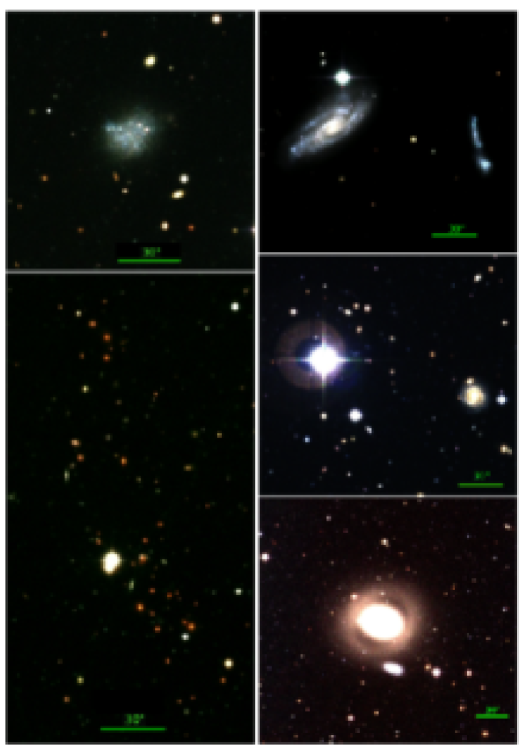
Figure 6: Color, BVR, enlarged view of some sources in the ESIS fields. North is up, East is left; a 30″scale is indicated.

Each one of the 22 ESIS WFI pointings consists of at least $\sim$30 science frames per band (B,V,R, see Table 3). While co-adding all these frames together, we have excluded all those images with seeing larger than $\sim 1.2$ $[$arcsec$]$, with the exception of pointing no. 6, for which few images are available. The FWHM of point-like sources (see next Sections), as measured by SExtractor (Bertin & Arnouts 1996) on the final images, is reported in the fourth column of Tab. 3.

Figure 4 shows the weight map obtained during co-addition of Field no. 2, R band. The darkest regions have about half the exposure coverage of the lightest ones, due to gaps between the CCDs and dithering. The weight value defined as the ratio $N_{imgs}/N_{tot}$ between the effective number of images covering the given pixel and the total number of frames belonging to the given ESIS pointing. The weight maps were used by SExtractor in object detection and noise calculation. Figure 5 shows the R-band image of WFI Field number 3; Figure 6 includes some zooms on colorful sources.

The coordinates of the objects detected on the final co-added R-band image of one WFI field are compared to GSC 2.2 sources in Fig. 7 (left panels). The r.m.s of the distribution of coordinate differences turns out to be $\sim 0.12$ $[$arcsec$]$ in $\alpha\cdot\cos\delta$ and $\sim 0.10$ $[$arcsec$]$ in $\delta$, similar to what found by Arnouts et al. (2001) and Momany et al. (2001). The top left panel of Fig. 7 includes also comparison of data to Gaussian distributions with the same variance $\sigma$. The central plot shows that 70, 80 and 90% of the sources are included within $\Delta$ of $\sim 0.13,\ 0.16$ and $0.20$ $[$arcsec$]$ respectively. Similar results are obtained for the B and V bands and the other pointings. In the bottom graph, coordinate differences are plotted against $(\alpha,\delta)$: no systematic trends are detected.

Relative astrometry (i.e. the difference between coordinates in the 3 bands) is very accurate, because the three monochromatic frames were registered to the same astrometric map, as mentioned above. The right panels of Fig. 7 show the behavior of B vs. R coordinates for one WFI pointing; r.m.s are below 0.05 $[$arcsec$]$. Similar results are obtained also for V band and the other fields.

The astrometric accuracy has been checked also in the regions of overlap between ESIS fields. The bottom right panel of Fig. 7 reports the result for GSC 2.2 sources: coordinates measured on each pointing are compared to those estimated on contiguous fields. The plot includes all the central six ESIS fields.

3.3 Catalog extraction

Source extraction and magnitude measurement were performed using the SExtractor software (Bertin & Arnouts 1996).

Thanks to the astrometric transformations described in Section 3.2, the B, V and R images of each WFI pointing are perfectly aligned (see Fig. 7) with each other. Therefore it is very easy to cross-correlate single band source lists and generate a 3-band catalog.

We ran SExtractor on a B+V+R image obtained by simply summing the three monochromatic frames belonging to each WFI field. A Gaussian-filtered image was used for detection, with a kernel matching the seeing. We use this first 3$\sigma$ detection on the BVR image to build a list of objects (ASSOC_LIST) to be extracted and measured on the individual monochromatic frames. In this way, spurious detections on individual images are also minimized.

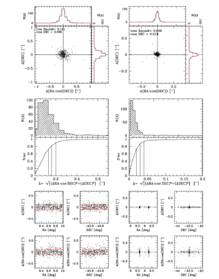
Figure 7: Astrometric accuracy of ESIS WFI data. Left panels: absolute R-band astrometric accuracy. The equatorial coordinates of ESIS sources are compared to those in the GSC 2.2 catalog. The central plot shows the distribution of $\sqrt{[\Delta(\alpha\cdot\cos\delta)]^{2}+[\Delta(\delta)]^{2}}$; the vertical lines include 70, 80 and 90% of the sources respectively. In the bottom left panel, the values of $\Delta(\alpha\cdot\cos\delta)$ and $\Delta(\delta)$ are plotted against $(\alpha,\delta)$. Right panels: relative astrometric accuracy. The coordinates measured on the B band image are compared to those in the R band. In the bottom right plot, the difference in coordinates among contiguous fields is shown, for common GSC 2.2 sources.

Photometry was then performed at 3$\sigma$ above background r.m.s. with SExtractor also. As a consequence of the dithering observing technique, regions along image borders and CCD gaps are covered by a small number of frames; weight maps (see Sect. 3.2) are used by SExtractor while detecting sources and computing magnitude uncertainties. Nonetheless, it is worth noting that magnitude uncertainties ($<$0.1 mag down to magnitude $\sim$25, for all the three bands) computed by SExtractor likely underestimate the real errors in photometric measurement, because they include only photon noise statistics (see tests in Section 4.2).

Table 3 reports the number of sources detected and measured by SExtractor on ESIS individual WFI frames. The total number of sources in pointings 1 to 6, is 132712, smaller than the sum on individual images because of overlap; the total number of objects on Fields 1-5 — full depth — is 118197.

Field no.	Number	3$\sigma$	FWHM
& filter	of frames	sources	[arcsec]
1 B	30	22999	1.008
1 V	28	18381	0.936
1 R	32	24006	0.960
2 B	25	18623	0.984
2 V	26	11780	1.176
2 R	30	19501	0.960
3 B	25	20385	0.984
3 V	30	18108	0.960
3 R	32	26118	0.912
4 B	30	18186	0.984
4 V	30	16016	1.056
4 R	30	23754	0.960
5 B	25	19835	0.936
5 V	25	15991	0.912
5 R	25	22564	0.876
6 B	10	14916	0.852
6 V	10	10441	0.912
6 R	10	14720	0.864

Table 3: Summary of source extraction. For each of the 6 ESIS WFI pointings analysed here, the total number of co-added frames, number of 3$\sigma$ extracted sources and FWHM of point-like objects are reported.

3.4 Photometric calibration

The fundamental requirement to be fulfilled by the ESIS service mode WFI program consisted of observing at least one OB (i.e. one set of 5 exposures, hereafter “reference OB”) per pointing, per band, during one photometric night. During the same photometric night, imaging of Landolt (1992) Ru149 or TPHE spectrophotometric standard fields — at similar airmasses — was performed. Eight different exposures were taken each time, in order to include the main standard stars on each individual CCD of the WFI array.

When combining $\sim$30 different images, belonging to various nights (see Tables 2 and 3), frames obtained with different sky conditions are mixed, hence the photometric information gets lost. Having a photometric reference night is necessary, to recover a correct calibration of magnitudes. The five images belonging to the reference OB were combined together and were used to determine the zeropoint shift $\Delta$mag$=$mag${}_{coadd}-$mag_ref, caused by the co-addition of $\sim$30 frames into the final frame.

The preliminary catalog (Sect. 3.3) was matched to the photometric conditions and normalized to unit airmass and exposure time, using the equation:

$$\textrm{mag}_{phot} = \textrm{mag}_{coadd}+2.5\log_{10}(t_{exp})$$

$$-K_{\lambda}\cdot A.M.-\Delta\textrm{mag}$$

where $A.M.$ is the average airmass of the reference OB, and $K_{\lambda}$ are the atmospheric extinction coefficients provided by ESO ($K_{b99}=0.23$, $K_{b123}=0.22$, $K_{v}89=0.11$, $K_{r162}=0.07$).

After pre-reduction and ss-flat correction of standard fields, color equations to transform instrumental magnitudes into the Johnson-Cousins system were computed for each CCD. The results are consistent with ESO official equations:

$$B_{J} = b_{99}+24.65+0.24\times(B_{J}-V_{J})$$

$$B_{J} = b_{123}+24.71+0.19\times(B_{J}-V_{J})$$

$$V_{J} = v_{89}+24.15-0.13\times(V_{J}-R_{C})$$ (16)

$$V_{J} = v_{89}+24.15-0.09\times(B_{J}-V_{J})$$

$$R_{C} = r_{162}+24.47\textrm{.}$$

The $b_{99}$ or $b_{123}$ equation is adopted depending on which filter was used (see Sect. 2).

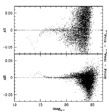
Figure 8: Self-check of photometric calibration. The color equations (Eqs. 16) built on three photometric bands, lead to two different solutions, based on the $(B-V)$ and $(V-R)$ colors. The magnitudes based on the two calibrations turn out to be perfectly consistent to each other.

The catalog was calibrated to the standard Johnson-Cousins photometric system ($B_{J}$, $V_{J}$, $R_{C}$), by solving the above array iteratively.

Since 3 bands and 2 colors are available, two different calibrations are possible, based on $(B-V)$ or $(V-R)$. Figure 8 shows the difference in magnitude between the two different calibrations. When one color was not available, a spiral-like average of 1.0 was adopted. Only B and V are shown in Fig. 8, since no color term affects the R band filter. The two estimates are self-consistent; the associated magnitude uncertainty is similar or even smaller than that estimated by SExtractor on background noise.

4 Quality tests

In order to test data quality and survey performance, a series of tests have been performed, based on simulations, aimed at determining:

• a semiempirical estimate of the effective depth reached and of completeness;

• a reliable estimate of magnitude uncertainty, overriding SExtractor’s;

• the reliability of SExtractor’s stellarity flag.

To this end, we have added synthetic sources to our images, by using IRAF tasks in the package artdata.

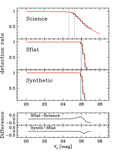
Figure 9: Detection efficiency of synthetic sources in the V-band. Three cases are studied: a real science frame already containing real objects, a ss-flat image and a totally synthetic sky frame (see text for further details). Histograms represent the real data, the continuous red line is a spline interpolation. Vertical dotted lines set the 97% and 90% limits. The bottom panel includes the difference in detection rate between the three cases.

The analysis comprises two steps. First we have tested three different types of images in order to understand the best way to reach our goal:

1. the real image, containing all real sources; we chose WFI pointing number 2, because it represents the worst case, containing a very bright ($V\sim 7.8$) star;

2. an empty image obtained from the non-smoothed ss-flat frame, built from 30 individual images belonging to the 6 ESIS central pointings;

3. a totally synthetic background image generated by IRAF, matching the r.m.s. properties of the real image.

This test was run on the V band and using point-like objects only; results are reported in Section 4.1. The best choice turned out to be the ss-flat frame, because it reproduces all the defects of real science images, but is not affected by confusion problems.

A number of different simulated images per band were then produced, by adding point-like, De Vaucouleurs or exponential disk objects onto the ss-flat. In each case, a different image was produced per 0.25 magnitude bin, in the range 20-27 mag. A population of 2000 sources was added in each case, for a total of $\sim$50000 objects on 14 different images per band.

Concerning De Vaucouleurs and disk profiles, intrinsic half-light radii between 2 and 10 $[$kpc$]$ and a Euclidean power law luminosity function were adopted. The artdata package assumes a redshift distribution that corresponds to the apparent magnitude distribution. The standard cosmological dimming of flux and angular size are applied to each artificial galaxy. Finally the synthetic objects are convolved with a gaussian kernel consistent with the real seeing of observations and are added to the ss-flat frames.

The results described below are based on SExtractor’s performance on this simulated images.

4.1 Detection rate

Figure 9 summarizes the results of the preliminary test performed on the V band images. The detection efficiency of SExtractor was defined as $\epsilon=N_{SEx}/N_{in}$, i.e. the fraction of input synthetic sources recovered by SExtractor. The three top panels in Fig. 9 show the dependence of $\epsilon$ on magnitude, measured on the real science final image, on the ss-flat frame, and on a synthetic sky image. The two bottom panels report the difference in $\epsilon$, between the various cases.

The effects of confusion influence the detection of synthetic sources on the real science frame, with respect to other cases, in two ways: $\epsilon$ decreases from unity at brighter magnitudes, because sources get lost in the halos of bright stars and very extended galaxies; $\epsilon$ decreases more slightly than in the other cases, because of spurious detection due to superimposition onto real sources.

Concerning the ss-flat image, which was intentionally neither smoothed, nor cleaned of bright halos, $\epsilon$ decreases less suddenly than on the synthetic sky, because some spurious sources are detected in the halos.

We estimate the amount of spurious detections by running SExtractor on the empty ss-flat (i.e. without any simulated object added), searching for sources at the positions of those previously detected. No spurious sources were detected down to V$\sim$25; at fainter fluxes about 1-2% of sources are not real, in the range 25-26 mag. Similar results were obtained in B and R.

Table 4 summarizes the resulting completeness values derived for point-like, De Vaucouleurs and exponential-disk simulations on the ss-flat images, in the three bands. Overall, a 90% detection efficiency is reached at mag$\sim$25.5, with some scatter, depending on the case. For pointing number 6, consisting of 10 exposures only, this limit is $\sim 0.5$ mag brighter.

Point-like sources
	R			V			B
mag	$\sigma$	s.i.q.	rate	$\sigma$	s.i.q.	rate	$\sigma$	s.i.q.	rate
21	0.024	0.005	0.999	0.024	0.003	0.999	0.022	0.002	0.999
23	0.063	0.034	0.999	0.042	0.020	0.999	0.033	0.015	0.999
25	0.283	0.175	0.999	0.199	0.115	0.999	0.158	0.095	0.999
26	0.478	0.266	0.064	0.291	0.178	0.953	0.282	0.172	0.980
Exponential-disk sources
	R			V			B
mag	$\sigma$	s.i.q.	rate	$\sigma$	s.i.q.	rate	$\sigma$	s.i.q.	rate
21	0.060	0.027	0.996	0.074	0.028	0.994	0.039	0.010	0.993
23	0.142	0.084	0.994	0.371	0.166	0.992	0.089	0.035	0.989
25	0.470	0.298	0.931	1.042	0.602	0.983	0.254	0.147	0.981
26	0.858	0.275	0.018	1.195	0.678	0.522	0.456	0.256	0.693
De Vaucouleurs sources
	R			V			B
mag	$\sigma$	s.i.q.	rate	$\sigma$	s.i.q.	rate	$\sigma$	s.i.q.	rate
21	0.064	0.033	0.998	0.084	0.038	0.997	0.035	0.014	0.997
23	0.182	0.102	0.993	0.446	0.210	0.994	0.082	0.042	0.990
25	0.512	0.291	0.811	1.148	0.658	0.976	0.322	0.181	0.974
26	0.829	0.327	0.009	1.218	0.701	0.268	0.455	0.279	0.443

Table 4: Summary of quality simulations on the ss-flat image. Three cases are reported, consisting of point-like, De Vaucouleurs and exponential-disk synthetic objects. For each band, magnitude standard deviation and semi-inter-quartile (s.i.q.) are listed, as well as extraction efficiency.

4.2 Magnitude uncertainty

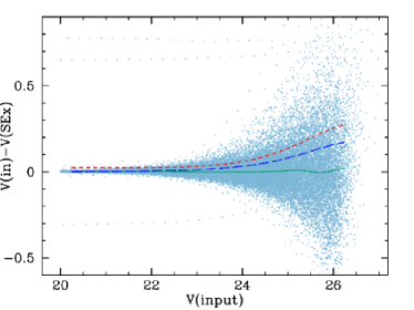
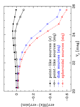
Figure 10: Top panel: V-band ss-flat simulation. Difference between the input magnitude of point-like synthetic sources and the value measured by SExtractor, as a function of input mag. The solid line traces the median, the short-dashed standard deviation, and the long-dashed semi-inter-quartile (s.i.q.). Bottom panel: comparison between the r.m.s. (or s.i.q.) computed on simulated data and the median magnitude uncertainty measured by SExtractor on real data, in a given magnitude bin. Solid, dotted and dashed lines represent point-like, disk and spheroidal sources, respectively.

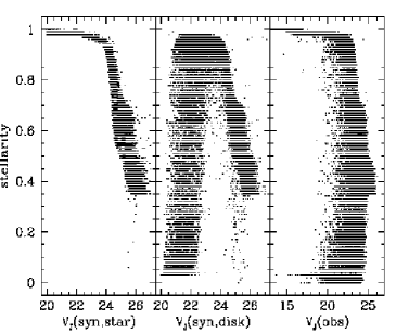
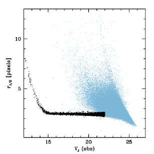
Figure 11: Left: dependence of the stellarity index on $V_{J}$ magnitude, for simulated point-like sources, simulated exponential disks and real data. The horizontal dotted line sets the CLASS_STAR$=$0.95 limit. Right: half-flux radius as a function of $V_{J}$ magnitude. The dark dots define the locus of point-like sources.

An estimate of magnitude uncertainties is obtained by comparing the input simulated fluxes and the measured values. The top panel in Fig. 10 shows the case of point-like sources added to the V band ss-flat frame: the difference between input and extracted magnitudes is plotted as a function of input magnitude. The solid line represents the median difference, the short-dashed line is the standard deviation from the median value and the long-dashed line traces the semi-inter-quartile.

The bottom panel in Fig. 10 compares the standard deviation and semi-inter-quartile of simulations (see top panel) to the median magnitude uncertainties measured by SExtractor on real data. The latter is computed as the median of uncertainties for all real sources in a given magnitude bin. In the case of point-like sources, SExtractor’s errors are compared both to the standard deviation from the median (filled circled) and to the semi-inter-quartile (open circles). The synthetic $\sigma$ is typically driven by outliers (such as unresolved double stars), while the semi-inter-quartile width of the distribution provides a fairer comparison to SExtractor’s uncertainties.

The estimate of magnitude errors for non-pointlike objects is compared to the simulated ones for disk and spheroidal galaxies (open squares and triangles respectively). The discrepancy between the two estimates is larger in this case, because of non-shot-noise effects like failure in detecting the faint wings of galaxy profiles or size dimming for the faintest sources.

Table 4 summarizes the results for all the cases studied. Typical uncertainties at mag$=21,\ 25$ are $\sim 0.03,\ 0.3$ in the B band, $\sim 0.05,\ 0.5$ in V and R. An uncertainty of 0.05 mag at 21 corresponds to one of 5% in flux, while 0.5 at 25 corresponds to 60% in flux.

4.3 Stellarity

Finally, the simulations described above are also useful to test the reliability of SExtractor’s stellarity flag. In combination with real data, it is possible to evaluate down to which magnitude the CLASS_STAR flag represents a realistic indication of the source profile.

The left plots in Fig. 11 show the distribution of CLASS_STAR as function of magnitude, for the simulated point-like sources (left panel), simulated exponential disks (central panel), and for the real data (right panel).

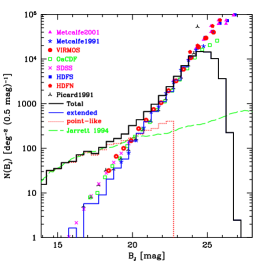
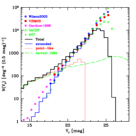
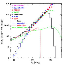
Figure 12: Observed ESIS number counts (histograms), compared to literature data (dots) and Jarrett et al. (1994) Milky Way model (long-dashed line). The ESIS data are split into extended (this solid histograms) and point-like (dotted) components. The bold solid histograms represents the total ESIS counts.

The plots suggest that a CLASS_STAR$>$0.95 is a good representation of point-like sources up to V$\sim 23$. Note that effectively no point-like sources are detected above this threshold, at fainter fluxes. Nevertheless, a significant contamination by galaxies is expected at fluxes fainter that V$\sim$21, as confirmed by Fig. 12 on real data (see also Section 5.1). Similar results are obtained in the other two bands, with slightly fainter magnitude limits.

An intrinsically wide scatter in CLASS_STAR is typical of galaxies. Moreover these tend to behave like point-like sources at faint fluxes, because the profiles of small objects are dominated by seeing.

A safer way of extracting point-like sources relies on the half-light radius, $r_{1/2}$, enclosing 50% of the object’s total flux. As for point-like sources $r_{1/2}$ depends only on the image seeing, when plotted against magnitude it defines a tight “stellar” locus (see the diagram on the right side of Fig. 11). Although still contaminated by QSOs, this method provides a good representation of point-like objects down to V$\sim 22$.

5 Source counts

The magnitude distribution of galaxies, per unit sky area, provides strong constraints on their evolutionary history (Ellis 1997; Metcalfe et al. 1995). In monolithic-collapse models (Eggen et al. 1962), the bulk of stars formed in early-type galaxies at very high redshift, and galaxies evolve passively to present day; while subsequent merging and star formation are limited. In a hierarchical merger scenario (Kauffmann & Charlot 1998), the bulk of the stars form in disk-like galaxies that later merge to become early-type galaxies. The luminosity and density of galaxies strongly evolve with cosmic time due to mergers and related starbursting events.

We build ESIS counts excluding WFI pointing number 6, hence including sources within a 1.22 $[$deg${}^{2}]$ area. Figure 12 shows the data: the solid thick histogram represents the total observed number counts, the dotted histogram the counts for point-like sources (see Sect. 4.3), and the thin solid histogram the counts for extended objects.

5.1 Star-galaxy separation

In order to compare to galaxy evolutionary models, stars must be removed from number counts. On the basis of the analysis presented in Sect. 4.3, the half-light radius $r_{1/2}$ provides a good representation of point-like sources, but this method is limited to magnitudes brighter than $\sim 22$. Moreover, it is worth to note that quasars are intrinsically point-like sources and cannot be a priori distinguished from stars, on the basis of BVR colors only.

The long-dashed line in Figure 12 represents the expected magnitude distribution for stars, based on the Milky Way model by Jarrett (1992) and Jarrett et al. (1994). These authors adopt a three component model, including a halo, a thin disk and a thick disk stellar population. This model reproduces the observed star counts in different galactic lines of sight, as well as SDSS data.

The Milky Way model is consistent with ESIS data at bright fluxes, in the B and V bands, while it seems to underpredict (by about 20-25%) star counts in the R band at magnitudes $<19$. Between magnitudes 21 and 22, observed pointlike counts still show some excess with respect to Jarrett model. This may be caused by residual contamination from faint unresolved galaxies or by a quasar component.

In what follows (e.g. Figure 13), two corrections will be applied to number counts for stars: one based on the Jarrett et al. (1994) model, the other using SExtractor’s identification. Overall the latter correction is more solid than the former at bright fluxes, while the former is most suitable for faint magnitudes. In any case it should be noted that the stellar contribution to the counts at the faint end (less than 3%) is almost negligible, when comparing data and galaxy evolutionary models, while it dominates the bright counts.

5.2 Comparison to literature data

Figure 12 also compares ESIS galaxy counts to a collection of literature data. In particular, HDFN (Williams et al. 1996), HDFS (Metcalfe et al. 2001), SDSS (Yasuda et al. 2001), VIRMOS deep survey (McCracken et al. 2003), OaCDF (Alcalá et al. 2004), NTT SUSI Deep Field (Arnouts et al. 1999). Additional data are from Metcalfe et al. (1991, 2001), Picard (1991), Wilson (2003) and Gardner et al. (1996). All magnitudes have been transformed to the Johnson-Cousins photometric system, adopting the appropriate relations (usually reported by authors).

ESIS number counts are generally consistent with the results from other surveys, in the common flux range. At bright magnitudes, some differences arise between our counts for extended sources (which can be considered galaxies for mag$<$18). This is particularly true in the V band, the Gardner et al. (1996) data being significantly higher than ESIS’, possibly due to a different choice in accounting for stars, or to cosmic variance.

5.3 Galaxy evolutionary models

Differential galaxy number counts can be described as the integral over cosmic time of the galaxy luminosity function (LF), in a specific flux bin (e.g. Franceschini et al. 2001; Guiderdoni & Rocca-Volmerange 1991). The shape and normalization of the LF is assumed constant in non-evolutionary models; galaxy luminosity evolves by means of galaxy ages, in pure luminosity evolution models (PLE); finally in complete evolutionary models, the LF changes as a function of redshift, for example due to enhanced star formation activity, triggered by encounters and mergers between galaxies.

In the recent years hierarchical clustering models have gained increasing popularity in the description of galaxy formation and evolution. Primordial density perturbations are amplified by gravitation and collapse to form almost virialized structures called dark matter (DM) haloes. In the cold dark matter (CDM) scenario (Peebles 1982; Blumenthal et al. 1984), smaller haloes form first, subsequently merging into bigger haloes. Gas cools down in the potential wells of the haloes, leading to the formation of stars and galaxies. The spectrophotometric evolution of stellar populations, combined with the history of stellar formation of galaxies, finally produce their observable properties: spectra, colors, etc. Semi-analytic modern models combine these and others ingredients and follow the various processes transforming the primordial power spectrum of density fluctuations into the spectral energy distributions of stellar populations and galaxies. (e.g. Hatton et al. 2003; Guiderdoni et al. 1998).

Figure 13 compares ESIS galaxy counts to the four different kinds of models. Galaxy counts are obtained from total number counts in two ways: by subtracting point-like identifications (open squares) and by using the Jarrett et al. (1994) model (stars). Poisson errors are smaller than the symbols, for mag$>$18.

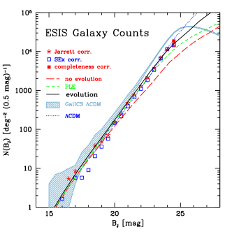
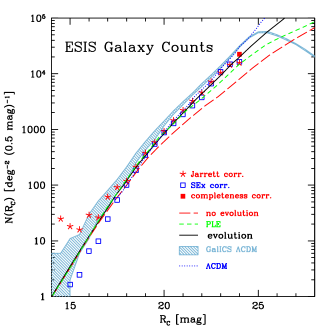
Figure 13: Comparison between ESIS galaxy counts and prediction of evolutionary scenarios. Open squares are number counts for extended sources (based on the half-flux radius analysis). Asterisks represent total galaxy counts corrected for stars contribution with the Jarrett et al. (1994) Milky Way model. Filled squares are data corrected for completeness (at the faintest fluxes). Models belong to Metcalfe et al. (2001), Nagashima et al. (2002) and the GalICS team (shaded area, Hatton et al. 2003).

	BJ		VJ		RC
mag	$\log N$	$\log N$	$\log N$	$\log N$	$\log N$	$\log N$
	(Ext.)	(Tot.)	(Ext.)	(Tot.)	(Ext.)	(Tot.)
16.0	0.215	1.713	0.391	1.926	0.817	2.011
16.5	0.215	1.848	0.759	1.922	0.993	2.044
17.0	0.692	1.935	1.090	2.041	1.432	2.228
17.5	0.759	1.900	1.294	2.128	1.740	2.348
18.0	0.993	2.014	1.654	2.277	2.004	2.443
18.5	1.345	2.152	1.943	2.406	2.272	2.600
19.0	1.567	2.228	2.171	2.524	2.544	2.791
19.5	1.752	2.329	2.460	2.704	2.743	2.945
20.0	2.164	2.508	2.612	2.838	2.949	3.099
20.5	2.359	2.652	2.849	3.014	3.114	3.260
21.0	2.596	2.820	3.023	3.159	3.275	3.412
21.5	2.836	2.996	3.184	3.312	3.433	3.562
22.0	3.050	3.184	3.386	3.479	3.582	3.703
22.5	3.275	3.386	3.584	3.641	3.828	3.887
23.0	3.540	3.621	3.815	3.820	4.043	4.047
23.5	3.834	3.864	3.997	3.997	4.183	4.183
24.0	4.077	4.078	4.120	4.120	4.350	4.350
24.5	4.271	4.271	4.224	4.224	–	–

Table 5: ESIS BVR number counts $[$deg${}^{-2}\ ($0.5 mag$)^{-1}]$. Completeness corrections has been applied, based on simulations of galaxy-like sources (see Sect. 4). Total and extended source counts are provided.

Completeness correction is attempted at the faintest fluxes, on the basis of the detection rate analysis carried out in Section 4. Only one magnitude bin can be fully recovered, reaching B,V$\sim$24.5 and R$\sim 24$. Table 5 lists the ESIS counts.

Describing the data as a power law

$$\log N\propto\gamma\times\textrm{mag,}$$ (17)

we find $\gamma_{B}=0.48$ in the range $B=19-24$, similarly to Ellis (1997) and Metcalfe et al. (2001). The V-band data can be fitted with a double power law, having an elbow at $V\sim 20$: $\gamma_{V}=0.56$ between 16 and 20, and $\gamma_{V}=0.37$ for $V=20-24$. Finally, concerning R band data, the galaxy counts are well reproduced by $\gamma_{R}=0.58$ in the range $16-20$ mag and $\gamma_{B}=0.32$ for $R=20-24$, consistent with Metcalfe et al. (2001). Models are compared to data only for B and R band, because — in the literature — the R band is usually preferred to the V band.

In Fig. 13, the long-dashed line represents the no-evolution model, by Metcalfe et al. (2001), obtained for a $q_{0}=0.5$ cosmology. These authors model the galaxy luminosity function (LF) as a Schechter function, with $\alpha=-0.7$ for E/S0/Sab galaxies, $\alpha=-1.1$ for Sbc spirals and $\alpha=-1.5$ for bluer Scd/Sdm ones. In the B-band the model was normalized to $B\sim 18$, instead of 15 (see Metcalfe et al. 1991, 1995, 2001, for a discussion in support of this choice) and reproduces reasonably well the observed counts down to $B\sim 21$. In the R band the consistency with data holds only to R$\sim 19.5$. At fainter fluxes the model quickly diverges from the ESIS counts.

The short-dashed line in Fig. 13 is a PLE model (Metcalfe et al. 2001), built assuming that the evolution of the different morphological types is governed by their star formation history. Exponentially decaying star formation rates are adopted (Bruzual & Charlot 1993), using $\tau=2.5$ Gyr for E/S0 and Sab galaxies and $\tau=9$ Gyr for other spirals types. Present day galaxy ages are $\sim 12.7$ Gyr, implying a formation redshift of $z_{f}=9.9$. This model is in good agreement with ESIS data down to B,R$\sim$23, after which the accordance fails.

Metcalfe et al. (2001) introduced a population of dwarf ellipticals to increase the model-predicted counts at the faintest fluxes (down to B,R$\simeq 28$, see also Ellis 1997) and match observations. Alternative solutions lead to equally good fits, for example merging evolutionary models.

The solid line in Fig. 13 represents an evolutionary model, with a LF slope of $\alpha=-1.75$ for blue Scd/Sdm galaxies at redshift $z>1$, steeper than the local $\alpha=-1.5$ (Metcalfe et al. 2001). This model provides a good fit to ESIS data over the entire magnitude range considered.

The GalICS (Galaxies In Cosmological Simulations, Hatton et al. 2003) project provides a hybrid model for hierarchical galaxy formation studies, combining large cosmological $N$-body simulations with semi-analytic recipes to describe the properties of galaxies within dark matter haloes. We have retrieved mock catalogs produced with the GalICS model, for a total of 10 different fields of 1 $[$deg${}^{2}]$, in order to take into account the cosmic variance of the mock catalogs.

GalICS simulations assume a $\Lambda$CDM flat Universe ($\Omega_{m}=0.333$, $\Omega_{\Lambda}=0.667$, $h=0.667$, $\sigma_{8}=0.88$). Each realization consists of a $100\leavevmode\nobreak\ h^{-1}$ $[$Mpc$]$ cube, containing $256^{3}$ particles of mass $8.272\cdot 10^{9}\ M_{\odot}$. The spatial resolution of the simulation is 29.29 $[$kpc$]$; the evolution of the Dark Matter density field is followed from $z=35.59$ to $z=0$, through 70 different snapshots.

Dark matter halos containing more than 20 particles (i.e. with $M\geq 1.66\cdot 10^{11}\ M_{\odot}$) are identified and their merging history trees are then computed. Baryons are evolved within these halo merging history trees, following a set of semi-analytic prescriptions (the Mock Map Facility, MoMaF, Blaizot et al. 2005) that account for (among other effects) heating and cooling of the gas within halos, star formation and supernovae feedback on the environment, evolution of stellar populations, metal enrichment, disk instabilities, tidal stripping, and formation of spheroids through galaxy mergers.

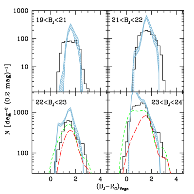
Figure 14: Observed $B_{J}-R_{C}$ color distribution. Left: extended sources. Overplotted are: a no-evolution (long-dashed line, Roche et al. 1996), a PLE (short-dashed, Roche et al. 1996) and GalICS $\Lambda$-CDM (shaded area, Hatton et al. 2003) models. Right: point-like sources, as compared to Jarrett et al. (1994) predictions for spheroid (dashed line) and disk (dotted line) stars.

The shaded regions in Fig. 13 represent the locus of predictions by the GalICS model, for the 10 different simulations considered. In the R band, consistency between model and observations holds at the brighter fluxes, but the model seems to overpredict galaxy number counts by at least $\sim$30% at magnitudes fainter than $\sim$20. In the B band, the discrepancy is more significant, model predictions overpredicting number counts by a factor of $\sim 1.5$ at $B_{J}>23$.

Nagashima et al. (2002) presented a $\Lambda$CDM semi-analytic model, which produces merger trees of Press-Schechter dark halos, in an $\Omega_{m}=0.3$, $\Omega_{\Lambda}=0.7$, $h=0.7$ Universe. This model includes the effects of dynamical response to supernova- and starburst-induced gas removal on size and velocity dispersions, which seems to play an important role in dwarf galaxy formation. The dotted line in Fig. 13 represents the Nagashima et al. (2002) model, which turns out to be fairly consistent with ESIS data in all bands, excepted for some excess in the number counts at faint fluxes.

Overall, the comparison of ESIS optical number counts to theoretical predictions favors a scenario in which the Universe has experienced an epoch with many encounters and interactions between galaxies, possibly at $z>1$, when the mean restframe UV-B luminosity of galaxies was larger than locally, because of enhanced star formation activity, likely triggered by mergers.

5.4 Color distributions

The distribution of observed colors, for both galaxies and stars, provides additional constraints to cosmic evolution and galactic models.

The left panel in Fig. 14 shows the distribution of the $B_{J}-R_{C}$ color for extended sources, in different $B_{J}$ magnitude bins. A non-evolutionary model (long-dashed line, Roche et al. 1996) systematically underpredicts the color counts, in the $22<B_{J}<24$ bins. The PLE model (short dashed, Roche et al. 1996) is more consistent with the data, but still does not reproduce observations in the faintest magnitude bin. Concerning the two brightest magnitude bins, only few model predictions of the observed-frame colors are available in literature. The GalICS $\Lambda$-CDM color histogram seems to be too much peaked and to predict more sources than observed (see also Fig. 13), in particular overestimating the number of faint blue galaxies.

The right panel in Fig. 14 compares the observed color distribution of point-like sources (defined as in Sect. 4.3) to the predictions of the Jarrett et al. (1994) Milky Way model. The dashed line refers to the spheroidal component, the dotted one to the disk population. Despite model predictions are fairly consistent to the observed point-like number counts (Fig. 12), the observed color distribution shows an excess of red sources at the faint fluxes and might caution against a residual contamination from unresolved galaxies.

6 Potential for multi wavelength investigations

The ELAIS-S1 field benefits from an extensive follow up carried out over the whole electromagnetic spectrum from X-rays to radio wavelengths (see also Fig. 1). In this Section we match ESIS data to catalogs in other spectral domains, with the purpose of showing some of the potential of multi-wavelength analysis of deep surveys.

6.1 Observations in ELAIS-S1 and match to ESIS data

The European Large-Area ISO Survey (ELAIS, Rowan-Robinson et al. 1999; Oliver et al. 2000), consisted of a deep, wide-angle survey at high galactic latitudes, with the Infrared Space Observatory (ISO). The primary ELAIS survey was carried out over 12 $[$deg${}^{2}]$, at 15 $\mu$m (with the ISOCAM camera, Cesarsky et al. 1996) and 90 $\mu$m (with ISOPHOT, Lemke et al. 1996); additional observations were performed in restricted areas at 6.7 and 175 $\mu$m, in collaboration with the FIRBACK team (Puget et al. 1999). The main survey area was divided into three fields in the northern hemisphere (N1, N2, and N3) and one field in the southern hemisphere (S1), which is the target of the ESIS survey.

The ELAIS-S1 field, centered at $\textrm{RA}=00^{h}34^{m}44^{s}.4$, $\textrm{DEC}=-43^{\circ}28^{\prime}12^{\prime\prime}.0$ (J2000.0), covers a sky area of about $2^{\circ}\times 2^{\circ}$ and includes the minimum in Galactic 100 $\mu$m cirrus emission in the Southern sky (Schlegel et al. 1998).

The ELAIS survey in the S1 field reached 1.0, 0.7 and 70 $[$mJy$]$ depth in the 6.7, 15 and 90 $\mu$m bands (Rowan-Robinson et al. 2004). No 175 $\mu$m observation was carried out in ELAIS-S1. The final 15 $\mu$m catalog contains 736 sources down to $\sim$1 mJy, $\sim$20% of which are stars (Vaccari et al. 2005).

Gruppioni et al. (1999) performed a radio (1.4 GHz) survey with the Australia Telescope Compact Array (ATCA), over 4 sq. deg. in the ELAIS-S1 area, producing a catalog (already public) of 652 sources, down to a minimum flux density of $\sim$0.2 mJy (5$\sigma$). The current 1.5 $[$deg${}^{2}]$ ESIS area contains 268 of the ATCA radio sources detected in ELAIS-S1, $\sim$65% of which have an optical counterpart. A deeper survey is in progress by B. Boyle and collaborators.

La Franca et al. (2004) presented spectroscopic and R-band data for 406 15 $\mu$m sources in the ELAIS-S1 field, over the flux density range $0.5<S(15\mu\textrm{m})<150$ $[$mJy$]$. The R band data were obtained by an ESO imaging campaign with the DFOSC instrument mounted on the 1.54 Danish/ESO telescope at La Silla (Chile), reaching 95% completeness level at R$\sim$22.5.

Spectroscopic observations of the optical counterparts of the ISOCAM S1 sources were carried out at the 2dF/AAT, ESO Danish 1.5 m, 3.6 m and NTT telescopes, adopting instrumental configurations with $\sim$10 Å resolution and covering the 4000-9000 Å wavelength range on average (La Franca et al. 2004).

Spitzer/SWIRE observations in ELAIS-S1 cover roughly the whole ISO region and a total sky area of $\sim$7 $[$deg${}^{2}]$, reaching 5$\sigma$ sensitivities of 3.7, 5.3, 48, 37.7 and 350 $\mu$Jy in the 3.6, 4.5, 5.8, 8.0, 24 $\mu$m channels respectively (Lonsdale et al. 2004). IRAC angular resolution spans $\sim$2.5 to 3 $[$arcsec$]$, while for the MIPS 24 $\mu$m band it is $\sim$6″. Data reduction was carried out by the Spitzer Science Center and SWIRE team. Absolute photometric uncertainty is $\sim$10% both for all bands. SExtractor’s Kron fluxes are considered for extended sources, while aperture photometry is used for point-like objects, corrected for aperture losses, as recommended by the Spitzer Science Center and SWIRE data release documentation (Surace et al. 2004). The astrometric accuracy of the SWIRE data products is $\sim$0.5″(after image reconstruction and comparison to 2MASS positions). The SWIRE band-merged catalog has been cross-correlated with ESIS WFI sources, by means of a simple nearest-match algorithm, adopting a radius of 1″; 71779 SWIRE sources lie in the ESIS WFI current area; 53267 matches (i.e. $\sim$74%) are found using this criterion.

About 40% of the ELAIS-S1 area was surveyed by BeppoSAX, down to a 2-10 keV sensitivity of $\sim$10^-13 $[$erg cm^-2s${}^{-1}]$ (Alexander et al. 2001). More recent XMM observations target the central area of the ISO field (Puccetti et al., in preparation). A mosaic of four deep XMM pointings covers $\sim$0.6 $[$deg${}^{2}]$ with the EPIC and two MOS cameras onboard XMM. The average net exposure time is $\sim$50 $[$ks$]$, in the energy range between 0.5 and 10 $[$keV$]$. WFI and XMM sources were cross-correlated if lying within a radius of 2″(close to the typical 1$\sigma$ XMM error box); 264 out of the 479 XMM sources are matched to ESIS objects.

The XMM ELAIS-S1 area is the target of further complementary observations. As part of ESO Large Programme 170.A-0143 (P.I. A. Cimatti, Dias et al., Buttery et al., in prep.), the ELAIS-S1 central $\sim$0.8 $[$deg${}^{2}]$ was the target of near-IR J and Ks imaging with SOFI on NTT, reaching J$<$21 and Ks$<$20 (Vega).

VIMOS/VLT spectroscopy was carried out in summer 2004 and 2005, in $2\times 33$ hour observing runs (73.A-0446 and 75.A-0428; PI: F. La Franca). The whole XMM-NIR area was the target of low resolution spectroscopy over the wavelength range 5000-9500 Å. During the first half of the survey, 1200 X-ray and $K_{s}<18.5$ galaxies were observed; in period 75 the targets consisted of 1000 X-ray sources plus 24$\mu$m SWIRE galaxies. R-band VLT pre-imaging provides additional data down to $R\sim 25$. Further spectroscopy of optically bright ($R<21$) X-ray and mid-IR sources is being performed at the 3.6m/ESO telescope, during Fall 2005. These data will be presented in future papers by F. La Franca and collaborators.

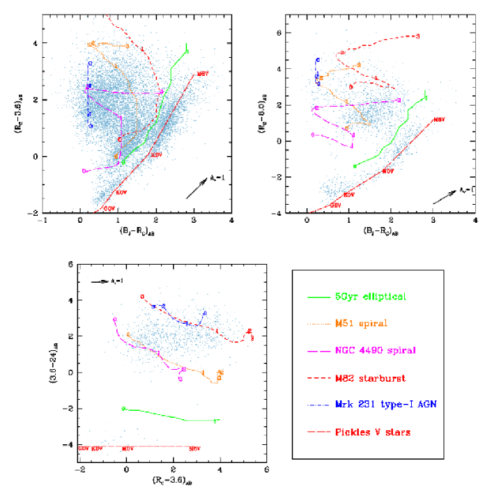
Figure 15: Color-color plots for ESIS sources matched to SWIRE/Spitzer objects. Template tracks represent k-corrected colors for different classes of sources, as a function of redshift ($z=0-3$). The class-V stellar track was obtained by extending the Pickles (1998) library to the infrared, assuming a Rayleigh-Jeans law. The reddening arrow refers to the standard extinction law by Cardelli et al. (1989).

The ultraviolet Galaxy Evolution Explorer (GALEX, Martin et al. 2005) Deep Imaging Survey (DIS) is observing $\sim$80 $[$deg${}^{2}]$ in 12 different areas, including ELAIS-S1 (Burgarella et al. 2005). Four ES1 GALEX tiles are already available to the public as part of data Release no.1 (GR1); two of these (namely tiles 00 and 01) match $\sim$0.93 $[$deg${}^{2}]$ of the ESIS-WFI area described here. The exposure times for these two tiles are $\sim$100 and $\sim$50 $[$ks$]$ respectively. The photometric catalogs in the far-UV (1344-1786 Å) and near-UV (1771-2831 Å) have been matched to ESIS data. In the ESIS-GR1 common area, 21025 GALEX sources were detected. The in-flight measured point-source FWHM is 4$\aas@@fstack{\prime\prime}$0 and 5$\aas@@fstack{\prime\prime}$6 in the two channels respectively. To be conservative, we used a matching radius of 2$\aas@@fstack{\prime\prime}$0 only, which is sufficient for our demonstrative purposes of showing the potential of observations in ELAIS-S1. In this way spurious and multiple matches are avoided. A more accurate match will be performed in the future, in order to provide as complete a multi-$\lambda$ study as possible. In this way, 17010 matches were found ($\sim$80%). We use the flux measurement provided by GR1.

6.2 Optical-IR colors

Color-color plots, built on a wide wavelength baseline turn out to be very useful to disentangle various classes of sources, different spectral domains being sensitive to different emission components.

Figure 15 shows three color-color plots including optical WFI, and mid-IR IRAC and MIPS photometric data. Synthetic tracks are overlaid on the data, as obtained by k-correcting template spectral energy distributions (SEDs) from $z=3$ to now. The solid curve belongs to a 5 Gyr old elliptical model (truncated at $z=1.2$, to be consistent with Universe age), the dotted line is a spiral M51-like model, the short-dashed line is a M82 prototype starburst template; these three models are built with the GRASIL code (Silva et al. 1998), and then upgraded by introducing observed PAH mid-IR features. The long-dashed line belongs to a semi-empirical SED of the blue peculiar spiral model of NGC 4490 (Polletta et al., in preparation) and the dot short-dash model belongs to the type-I AGN Mrk 231 (Fritz et al., in prep.). Finally the dot long-dash line belongs to class V stars and is obtained by extending the Pickles (1998) models to the infrared assuming a Rayleigh-Jeans law.

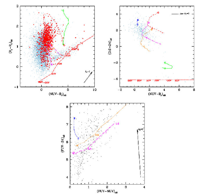
Figure 16: Color-color plots for GALEX ultraviolet sources in the ESIS current area. Template tracks are the same as in Fig. 15. The thick dots in the left top panel represent sources detected in the 24 $\mu$m Spitzer channel. The reddening arrow refers to the standard extinction law by Cardelli et al. (1989).

IRAC data, when combined with the optical, turn out to be a powerful tool to identify AGNs, normal galaxies, and stars. In the case of AGNs, the near-IR emission is dominated by a dusty torus heated by the central engine, while for normal galaxies, IRAC detects star light. Consequently, type-1 AGNs have flatter optical-NIR slopes and bluer colors; these kind of sources occupy a small characteristic locus in color space, while galaxy colors vary significantly as a function of redshift. The optical-IRAC color-color diagrams are only partially effective in disentangling galaxies and stars. In fact, stars and ellipticals tend to have similar colors at the $B-R$ reddest end, i.e. for high redshift ellipticals and cool stars, because the spectral continuum in early-type galaxies is dominated by old stellar populations.

Those color-color diagrams that include MIPS 24 $\mu$m data would be potentially very useful to further distinguish between different object classes, but SWIRE imaging is not deep enough to detect many normal galaxies at 24 $\mu$m. This is particularly true for elliptical galaxies.

6.3 Ultraviolet sources

Ultraviolet light is mainly emitted by young hot stars in galaxies, especially during star formation events. Nonetheless, powerful starbursts are typically hosted by dusty, thick environments (molecular clouds); in these cases, the UV emission of young stars is heavily extinguished and reprocessed to the mid- and far-IR.

The spectral energy distribution of type-1 AGNs contains a significant feature in the far-ultraviolet to optical region, known as “the big blue bump”. This feature is usually explained as the thermal emission from the optically thick accretion disk feeding the central massive black hole (e.g. Shields 1978; Malkan & Sargent 1982), which should peak in the extreme ultraviolet (EUV, $100<\lambda<912$ Å, e.g. Mathews & Ferland 1987).

The GALEX deep catalog in the ESIS area contains $\sim$19000 near-UV (1771-2831 Å) and $\sim$9000 far-UV (1344-1786 Å) sources. Roughly 7500 objects are detected both in the NUV and FUV channels. GALEX flux densities are typically brighter than $\sim$1 $[\mu$Jy$]$ in both bands.

As a result of the cross-correlation between multiwavelength catalogs described above, 856 sources turn out to be detected both by the NUV GALEX survey and the MIPS 24 $\mu$m channel; 803 of these have a secure optical counterpart, detected in all the three B, V, and R ESIS bands.

The left top panel in Fig. 16 represents the distribution of sources in the $(B-R)$ vs. $(NUV-B)$ color space. Overlaid are the same template tracks as in Fig. 15, truncated at a redshift of 1.5. Galaxies and stars are properly distinguished, the latter having $(NUV-B)>2$ and $B-R<1.5$. The Type-1 AGN template occupy a very small area in color space, near to $(NUV-B)=(B-R)=0$. For redshifts smaller than 1, the starburst template (dashed line) traces the area with $2<(NUV-B)<4$ and increasing $(B-R)>1$; at larger redshift, the $(B-R)$ color decreases again and the M82-like templates intersects the locus of $z<1$ spiral galaxies.

Apart from stars, the bulk of observed sources lies blueward of normal spiral galaxies. These are likely blue galaxies detected by GALEX thanks to some moderately enhanced, unobscured star formation, or type-1 AGNs. The locus of $z<1$ starbursts is not very populated, since dust extinction allows only the brightest sources to be detected in the UV.

The thicker points in the left top panel of Fig. 16 represent sources detected not only in the UV, but also at 24 $\mu$m by Spitzer. The right top panel of Fig. 16 compares the NUV and mid-IR excesses for these objects and include also a few stars (at bottom).

It is worth noticing that, once more, the introduction of 24 $\mu$m data is critical in disentangling different kind of sources. Template tracks nicely trace the increase of ongoing star formation from normal spirals to starbursts.

The bottom panel of Fig. 16 shows the ratio of mid-IR and far-UV fluxes as a function of the UV color of GALEX-24$\mu$m sources. The M82 starburst template lies above $(FUV-24)>8$: GALEX is not sensitive to young stars enshrouded in thick dusty clouds, which instead are detected in the mid-IR domain, thanks to dust reprocessing of the extinguished light. Blue UV galaxies with some 24 $\mu$m excess emission populate the upper part of the diagram (reddest $[FUV-24]$), in between the normal spirals and starbursts loci.

These color-color diagrams suggest that the majority NUV+MIPS sources are low or moderate redshift late-type galaxies ($z\leq 0.5$), with enhanced star formation activity. This ongoing star formation is almost unextinguished, or moderately absorbed ($A_{V}<0.5$), since both an ultraviolet and a mid-infrared excesses are detected in the SEDs of these galaxies.

6.4 SEDs examples

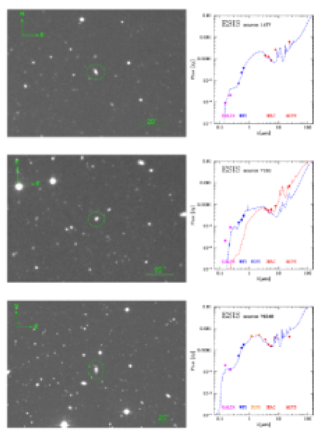
Figure 17: Spectral energy distributions of three sample sources, from the UV to the mid-IR. The superimposed templates are: 1477, spiral galaxy at $z=0.5$; 7160, starburst (dot-dashed line) and blue spiral (dashed) at $z=0.8$, 76348 spiral galaxy at $z=0.18$.

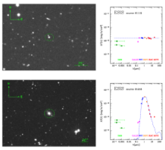
Figure 18: Spectral energy distributions of two X-ray detected sources. Object 81115 has a typical type-1 AGN SED; the optical emission from source 81218 is reproduced by an elliptical galaxy template at $z=0.2$ (dashed line).

Multiwavelength coverage from the X-rays to the far-IR allows the study of the nature of individual sources.

Blue optical restframe emission is dominated by young stars, while redwards (V, R bands), moderate-aged (type A-F) stars are preferentially detected.

Near-IR imaging traces the old stellar population of normal galaxies, and at $\lambda>4\ \mu$m, hot ($T\sim 1000$ $[$K$]$) dust emission, if present, is no longer negligible (e.g. in a AGN-heated torus).

Mid-IR radiation (5-30 $\mu$m) is dominated by warm ($T\sim 100-300$ $[$K$]$) dust, either heated by young stars in starburst galaxies or belonging to AGN tori. Polycyclic Aromatic Hydrocarbons molecules characterize mid-IR restframe light: bright emission bands are detected at 3.3, 6.2, 7.7, 8.6 and 11.3 $\mu$m and are typical of starburst galaxies.

In the far-IR spectral domain (30-200 $\mu$m), warm ($T\sim 100-300$ $[$K$]$) and cold ($T\sim 40$ $[$K$]$, belonging to cirrus) dust contribute to the energy budget, producing very bright luminosities in active galaxies (starbursts, AGNs) as well as in normal spirals.

Ultraviolet emission comes from young stars, but is extinguished by dust and reprocessed to the infrared (see also previous Section). Elliptical galaxies produce a significant “UV excess”, with regards to old stellar continuum, due to the presence of evolved components such as planetary nebulae and AGB manquè stars (see, for example, O’Connell 1999).

In the X-rays, AGN power-law emission is detected, either direct (type-I sources) or partially absorbed (type-II) in addition to scattered light (if the optical depth is high). Starburst galaxies host several X-ray components (see, e.g., Persic & Rephaeli 2002), most prominently thermal emission by X-ray binaries. Hot plasma in galaxy clusters produces extended thermal bremsstrahlung X-ray radiation.

Finally, adding deep radio observations will provide further insights into the nature of the ESIS galaxy populations, detecting synchrotron radiation from starbursts and radio loud AGN.

Figures 17 and 18 show the SEDs of five ESIS nearby sources, exemplifying different classes of objects. None of these sources were detected by ISO, nor by SWIRE’s 70 and 160 $\mu$m observations.

Source no. 1477 is a typical spiral galaxy with some enhanced, absorbed, ongoing star formation, displaying a moderate mid-IR excess in Spitzer’s 8.0 and 24 $\mu$m channels, and red UV-optical colors. Overlaid is a M51 spiral template shifted to $z=0.5$.

Source no. 7160’s SED resembles a blue starburst, showing a bright IR excess, likely powered by warm dust and PAH features, and moderately blue optical colors. The overlaid dashed line is a blue spiral template based on the nearby galaxy NGC4490 (Polletta et al., in prep.) shifted to $z=0.8$, while the dot-dashed line represents a M82 template at the same redshift, which reproduces the observed IR excess fairly well. The M82 template emission seems to be too absorbed in the optical-UV, being systematically fainter than the observed fluxes. This effect indicates that this source probably hosts a moderately extinguished starburst.

Object no. 76348 is a normal spiral galaxy, with some weak unextinguished ongoing star formation producing some UV excess. This source lies in the area observed with SOFI in the J and Ks bands. The dashed line is a M100 template, redshifted to $z=0.18$.

Figure 18 shows two objects detected in the X-rays and in the near-IR: a type-I AGN (81115) and a spheroidal galaxy (81218). The former SED is a flat power-law spectrum ($\lambda F(\lambda)=\textrm{{\em const}}$) over the entire wavelength range considered. The latter source shows some 24 $\mu$m emission in excess to what is predicted for a simple old stellar population (the dashed line represents an elliptical galaxy template at $z=0.2$), possibly powered by a hidden AGN, which is responsible also for the X-ray flux. Note that the presumably high UV-optical extinction of the possible type-2 AGN is confirmed by the quite hard X-ray spectrum. These plots report $\lambda F(\lambda)$ instead of flux density, in order to better highlight the energy budget in the X-rays, compared to the other wavelengths.

7 Summary

Optical B, V, R imaging of 1.5 square degree in the ELAIS-S1 area, belonging to the ESIS survey has been presented. The data consist of deep Wide Field Imager (2.2m ESO/MPI telescope in La Silla) observations, requiring $\geq$30 different frames per WFI pointing, for a total exposure time of 2.5h per band. Ad hoc technical solutions have been developed for correcting illumination gradients by means of super-sky flat fields, and to remove color effects and astrometric distortions. Accurate simulations have been run in order to estimate source extraction efficiency and photometric uncertainties.

A total of 132712 sources are detected on the 1.5 $[$deg${}^{2}]$ area analyzed here. Equatorial coordinates of objects are constrained within a $\sim$0.15 $[$arcsec$]$ r.m.s. uncertainty, with respect to the GSC 2.2 catalog; flux errors are estimated to be of the order of $\sim$2, 10, 20% at mag. 20, 23, 24; we reach 95% completeness B,V$\sim$25 and R$\sim$24.5.

Number counts in the B and R bands were compared to literature data and theoretical models of galaxy evolution. Our data are consistent with previous works from various surveys (e.g. HDFN, HDFS, VIRMOS, Williams et al. 1996; Metcalfe et al. 2001; McCracken et al. 2003). The stellar contribution to the counts has been taken into account both using SExtractor’s stellarity index and the Jarrett et al. (1994) Milky Way model. Comparison to number count models by Metcalfe et al. (2001), semi-analytical $\Lambda$CDM mock catalogs (GalICS Hatton et al. 2003) and $\Lambda$CDM (Nagashima et al. 2002) predictions confirm the need of galaxy luminosity evolution to properly reproduce the observed data. ESIS galaxy number counts suggest that at $z>1$ the rate of galaxy encounters was probably larger than today, and the mean restframe UV-Blue luminosity of galaxies was larger than locally, because of enhanced star formation activity, possibly triggered by mergers.

The ESO-Spitzer Imaging extragalactic Survey is providing optical identifications, colors, rough morphologies, photometric redshifts, for a good fraction of the $\sim 300000$ IR sources detected by SWIRE/Spitzer ($\lambda=$3.6, 4.5, 5.8. 8.0, 24, 70, 160 $\mu$m) in the 5 $[$deg${}^{2}]$ ELAIS-S1 area.

In addition to the Spitzer/SWIRE survey, ancillary data include observations in the X-rays (XMM, Puccetti et al., in prep.), ultra-violet (GALEX, Martin et al. 2005), near-IR (NTT, Dias et al., Buttery et al., in prep.), and radio (ATCA, Gruppioni et al. 1999) spectral domains. Some of the enormous potential stored in this multi-wavelength dataset has been traced in the last Section of this paper.

Thanks to the wide wavelength baseline covered, Spitzer-optical color-color diagrams turn out to be very powerful tools to disentangle different source populations, such as normal spirals, elliptical galaxies, starbursts and active galactic nuclei.

The ultraviolet to mid-IR color space was analyzed, matching ESIS sources to the GALEX Deep Imaging Survey catalog released in January 2005. Roughly 80% of the UV sources in the ESIS area are detected in the optical, while only a small fraction have a mid-IR 24 $\mu$m Spitzer counterpart. UV-optical and UV-24$\mu$m color-color diagrams suggest that sources detected both by GALEX in the ultraviolet and by MIPS at 24 $\mu$m are low or moderate redshift late-type galaxies, with enhanced, almost unextinguished ongoing star formation activity.

Finally, X-ray to far-IR spectral energy distributions of some ESIS sources were presented as examples of the characterization of SWIRE objects, based on ancillary data.

Such a comprehensive wavelength coverage of a large area will give a significant contribution, among others, in: (1) deriving the physical properties (e.g. ongoing rate of star formation and assembled stellar mass) of Spitzer galaxies up to $z\sim 3$, (2) searching for distant ($z>1$) galaxy clusters, (3) studying the statistical properties (e.g. number counts) of starburst, evolved galaxies, AGNs and comparing them to theoretical models, (4) studying the cosmic star formation density as a function of redshift, (5) building the luminosity and mass functions of galaxies and studying their dependence on redshift and environment.

Updates on the ESIS project are available on the web page http://dipastro.pd.astro.it/esis. The data described in this paper are included in the third SWIRE Spitzer Legacy data release (Fall 2005).