Comptonisation of CMB Photons in Dwarf Spheroidal Galaxies

Abstract

We present theoretical modelling of the electron distribution produced by annihilating neutralino dark matter in dwarf spheroidal galaxies (dSphs). In particular, we follow up the idea of Colafrancesco (2004) and find that such electrons distort the cosmic microwave background (CMB) by the Sunyaev-Zeldovich effect. For an assumed neutralino mass of 10 GeV and beam size of $1^{\prime\prime}$, the SZ temperature decrement is of the order of nano-Kelvin for dSph models with a soft core. By contrast, it is of the order of micro-Kelvin for the strongly cusped dSph models favoured by some cosmological simulations. Although this is out of reach of current instruments, it may well be detectable by future mm telescopes, such as ALMA. We also show that the upscattered CMB photons have energies within reach of upcoming X-ray observatories, but that the flux of such photons is too small to be detectable soon. Nonetheless, we conclude that searching for the dark matter induced Sunyaev-Zeldovich effect is a promising way of constraining the dark distribution in dSphs, especially if the particles are light.

1 Introduction

Dwarf spheroidal galaxies (dSphs) are important probes of dark matter. They are among the highest mass-to-light systems known, and the dynamics of their sparse stellar populations is governed by the dominant dark matter distribution. In addition, no emission has been detected from dSphs in wavebands other than the optical, indicating a lack of internal dust or gas (Fomalont & Geldzahler, 1979; Bonanos et al., 2004).

Here, we consider the distortion of the cosmic microwave background (CMB) by the non-thermal population of secondary electrons generated by dark matter annihilation. This is an example of the Sunyaev-Zeldovich (SZ) effect (Zeldovich & Sunyaev, 1969). Since we are dealing with electrons produced from dark matter annihilation, we write the distortion as the dSZ effect. Ensslin & Kaiser (2000) and Colafrancesco et al. (2003) calculated the signal expected from the SZ effect of a relativistic plasma, while Colafrancesco (2004) determined the dSZ effect in galaxy clusters.

As first pointed out in Colafrancesco (2004), dSphs are attractive targets because they have very high mass-to-light ratios and because they have few contaminants. In particular, they have little or no internal magnetic field, so it is not possible for synchrotron emission (from annhilation electrons or otherwise) to contaminate the dSZ effect. Since dSphs are believed to be almost devoid of interstellar gas, other mechanisms such as HI or CO line emission will not be important. CMB distortions are therefore a rather clean method to detect the annihilation signature. We therefore use existing models of the dark matter distribution in dSphs, and a possible form of the energy spectrum of electrons produced by dark matter annihilation, to derive the temperature change in the CMB. We focus on dark matter models explicitly constrained by observations, rather than simulations.

For our predictions, we assume that the cold dark matter particle is the lightest supersymmetric particle, the neutralino (Jungman, Kamionkowski & Griest, 1996). Current limits on the neutralino mass $M_{\chi}$ and centre-of-mass velocity-averaged cross-section $\langle\sigma V\rangle_{A}$ have been reviewed recently by Bertone, Hooper & Silk (2005). Based on these results, and considerations of current or upcoming experiments, we investigate the SUSY parameters $\langle\sigma V\rangle_{A}=10^{-26}\ \mathrm{cm^{3}s^{-1}}$ and $M_{\chi}=10\ \mathrm{GeV}$. Such low mass particles may provide a sizeable contribution to the matter density in the Universe (Bottino, Fornengo & Scopel, 2003), and hence are worthy of consideration. However, some dark matter candidates – such as the neutralino in the most commonly studied minimal supersymmetric models or the lightest Kaluza-Klein particle – must be more massive than this. The value assumed for $\langle\sigma V\rangle_{A}$ is consistent with the expected relic density in a Universe with $\Omega_{m}=0.3$ and $H_{0}=70\mathrm{kms^{-1}Mpc^{-1}}$ (Colafrancesco & Mele, 2001).We derive the dependency of dSZ signal on $\langle\sigma V\rangle_{A}$ and $M_{\chi}$, and show that the brightness temperature decrement $\Delta T_{B}\propto\langle\sigma V\rangle_{A}M_{\chi}^{-3}$. We initially calculate the expected signal for this optimistic choice of dark matter parameters.

The format of the paper is as follows. In Section 2, we discuss our dSph dark halo models, based on current work in the literature. We then discuss possible products of dark matter particle annihilation in Section 3. Observational consequences of such annihilation events are presented in Section 4. We conclude in Section 5.

2 Dwarf Spheroidal Models

With spherical symmetry of the dark halo assumed, we use the results of Evans, Ferrer & Sarkar (2004), who fit observational data on the Draco dSph (currently orbiting the Milky Way) from Wilkinson et al. (2004) to two sets of models via the Jeans equation (Binney & Tremaine, 1987).

2.1 Cusped Halo Models

Cusped halo models (CHMs)are favoured by numerical simulations, as reported by Navarro, Frenk & White (1997) (NFW) and Moore et al. (1998)). Using arguments based on the survivability of kinematically cold substructure, Kleyna et al. (2001) argued against a cusped halo for at least the Ursa Minor dSph. For the rest of the dSphs, cusped halos remain viable. We therefore consider number density radial profiles of the form

$$n\left(\hat{r}\right)=n_{0}a\left(\hat{r}\right),$$ (1)

where $n_{0}=Ar_{s}^{-3}/M_{\chi}$, and $a\left(\hat{r}\right)=\hat{r}^{-\gamma}\left(1+\hat{r}\right)^{\gamma-3}$, with $\hat{r}=r/r_{s}$. Table 1 gives the cusp slope $\gamma$, the scale radius $r_{s}$, the tidal radius $r_{t}$, and the overall normalisation $A$. The model is truncated at $r_{t}$, whose value depends on the Milky Way dark halo model.

Table 1: List of CHM model parameters for the Draco dSph. Values for $r_{t}$ in parentheses are for NFW models of the Milky Way, as opposed to isothermal power-law models which are without brackets.

$\gamma$	$\mathrm{A}\times 10^{7}M_{\odot}$	$r_{s}/\mathrm{kpc}$	$r_{t}/\mathrm{kpc}$	$M(r_{t})/10^{8}M_{\odot}$
0.5	2.3	0.32	6.6 (1.5)	5.5
1.0	3.3	0.62	7.0 (1.6)	6.6
1.5	2.9	1.0	6.5 (1.5)	5.5

To address the problem of the divergent central density in this model, we use the arguments of Blasi & Colafrancesco (1999) and Tyler (2002). The density profile is truncated at a radius $r_{\rm min}$, where we assume the dark matter annihilation rate matches the collapse timescale of the cusp. With this assumption, a small constant density core is created with radius $r_{\rm min}$

$$r_{\rm min}=r_{t}\langle\sigma V\rangle^{1/2}_{A}\left(\frac{n_{\rm min}}{4\pi GM_{\chi}}\right)^{1/4},$$ (2)

where $n_{\rm min}$ is the number density at the location of the constant density region. At small radii, Eq.(1) reduces to $n(r)\simeq AM^{-1}_{\chi}r^{-3}_{s}\hat{r}^{-\gamma}$, and hence we find:

$$r^{1+\gamma/4}_{\rm min}=r_{t}\langle\sigma V\rangle^{1/2}_{A}\left(\frac{Ar^{\gamma-3}_{s}}{4\pi GM^{2}_{\chi}}\right)^{1/4}.$$ (3)

Typically, $r_{\rm min}\sim 10^{13}\mathrm{m}$, and for such a small value, it is unlikely that tidal forces (from M31 or the Milky Way) could disrupt the central cusp. It should be noted that the Moore profile ($\gamma=1.5$) represents an extreme case for the inner slope of the cusp. Recent numerical simulations (e.g. Navarro et al, 2004; Diemand, Moore & Stadel, 2004) point towards a milder density slope of $\gamma\simeq 1.1$. However, we retain the Moore profile here as the models satisfy the observational constraints from stellar radial velocities. In addition, this profile allows an upper limit of the magnitude of the dSZ effect, enabling a broad yet well motivated parameter space to be investigated.

2.2 Cored Power-Law Models

The second family of dark halo profiles studied are the cored power-law (CPL) models (Evans, 1994). Again, these satisfy the Draco velocity dispersion observations, and take the form

$$n\left(\hat{r}\right)=n_{0}b\left(\hat{r}\right),$$ (4)

where $n_{0}=v^{2}_{a}/4\pi Gr^{2}_{c}$. The radial dependence is given by

$$b\left(\hat{r}\right)=\frac{3+\hat{r}^{2}\left(1-\alpha\right)}{\left(1+\hat{r}^{2}\right)^{2+\alpha/2}},$$ (5)

where $\hat{r}=r/r_{c}$. Table 2 gives the slope $\alpha$, the core radius $r_{c}$, the tidal radius $r_{t}$ and the velocity scale $v_{a}$. The dSph dark halo extends out to $r_{t}$, the value of which again depends on the model (isothermal power-law or NFW) used for the Milky Way.

Table 2: List of CPL model parameters for the Draco dSph. Values for $r_{t}$ in parentheses are for NFW models of the Milky Way, as opposed to isothermal power-law models which are without brackets.

$\alpha$	$v_{a}/\mathrm{km\ s}^{-1}$	$r_{c}/\mathrm{kpc}$	$r_{t}/\mathrm{kpc}$	$M(r_{t})/10^{8}M_{\odot}$
0.2	24.7	0.25	6.2 (1.3)	4.6
0	22.9	0.23	7.8 (1.4)	9.5
-0.2	20.9	0.21	10.1 (1.6)	22.43

3 Dark Matter Annihilation

Having established a set of representative dark matter halo models for dSphs, which embrace a range of possible structures, we determine the decay products of annihilating neutralinos. Electrons produced in this fashion have an associated cooling function $b\left(E\right)$, comprised of synchrotron losses, inverse Comption scattering (ICS) and Coulomb losses (Colafrancesco, 2004):

$$b\left(E\right)=\left(\frac{{\mathrm{d}}E}{{\mathrm{d}}t}\right)_{\rm syn}+\left(\frac{{\mathrm{d}}E}{{\mathrm{d}}t}\right)_{\rm ICS}+\left(\frac{{\mathrm{d}}E}{{\mathrm{d}}t}\right)_{\rm Coul}\mathrm{\ GeV\ s^{-1}}.$$ (6)

At electron energies $E\geq 150\mathrm{MeV}$ (Blasi & Colafrancesco, 1999), this function is dominated by the first two terms, so the Coulomb term may safely be dropped from the cooling function. In addition, there is no evidence in favour of significant magnetic fields in dSphs (Fomalont & Geldzahler, 1979). We therefore also drop the synchrotron cooling term, leaving (Colafrancesco & Mele, 2001)

$$b\left(E\right)=2.5\times 10^{-17}\times E^{2}\mathrm{\ GeV\ s^{-1}}.$$ (7)

Energy losses are efficient in the dSph halo, and dark matter annihilation from infalling material continuously refills the electron spectrum. In a first approximation, it seems reasonable to neglect diffusive effects, as dark matter annihilation replenishes the electron spectrum efficiently, at least in the central parts of the dSph.

Furthermore, we consider the dark matter to maintain a constant radial profile on the timescale of dark matter annihilation. This means that any time-variation of the electron distribution is negligible. The source function of electrons, $Q_{e}\left(E,r\right)$, generated in this fashion therefore obeys the stationary diffusion-loss equation (see, for example, Longair 1994)

$$\frac{\partial}{\partial E}\left(\frac{\mathrm{d}n_{e}\left(E,r\right)}{\mathrm{d}E_{e}}b\left(E\right)\right)=-Q_{e}\left(E,r\right),$$ (8)

which we integrate to obtain the annihilation-produced electron energy distribution $\mathrm{d}n_{e}\left(E,r\right)/\mathrm{d}E_{e}$:

$$\frac{\mathrm{d}n_{e}}{\mathrm{d}E_{e}}\left(E,r\right)=-\frac{1}{b\left(E\right)}\int Q_{e}\left(E,r\right)\mathrm{d}E.$$ (9)

The source function itself results from annihilation products of neutralino collisions. In this calculation, we follow the work of Tyler (2002), who used the Hill (1983) formula to determine the densities of particles produced by dark matter annihilation. Quark pairs and their subsequent fragmentation lead to pions as the main annihilation products. The primary decay particles are neutral pions, which decay to gamma rays, and charged pions, which decay as

$$\pi^{+}\rightarrow\mu^{+}\nu_{\mu}\ \mathrm{and}\ \pi^{-}\rightarrow\mu^{-}\bar{\nu}_{\mu}.$$ (10)

The muons then decay to electrons via

$$\mu^{+}\rightarrow e^{+}\bar{\nu}_{\mu}\nu_{e}\ \mathrm{and}\ \mu^{-}\rightarrow e^{-}\nu_{\mu}\bar{\nu}_{e}.$$ (11)

The number spectrum of electrons from a single $\chi\chi$ annihilation is then given by:

$$\frac{\mathrm{d}N_{e}}{\mathrm{d}E_{e}}=\int^{M_{\chi}}_{E_{e}}\int^{E_{\mu}/\bar{r}}_{E_{\mu}}W_{\pi}\frac{\mathrm{d}N^{(\pi)}_{\mu}}{\mathrm{d}E_{\mu}}\frac{\mathrm{d}N^{(\mu)}_{e}}{\mathrm{d}E_{e}}\mathrm{d}E_{\pi}\mathrm{d}E_{\mu},$$ (12)

where $\bar{r}\equiv\left(m_{\mu}/m_{\pi}\right)^{2}$, and the charged pion multiplicity per annihilation event is

$$W_{\pi}=\frac{4}{3}\frac{15}{16M_{\chi}}\left(\frac{E_{\pi}}{M_{\chi}}\right)^{-3/2}\left(1-\frac{E_{\pi}}{M_{\chi}}\right)^{2},$$ (13)

where the factor of $4/3$ accounts for the fact that annihilation electrons are only produced by charged pions, and that quarks (which eventually decay to charged pions) are produced in pairs. The number spectrum of muons produced per charged pion decay is

$$\frac{\mathrm{d}N^{\pi}_{\mu}}{\mathrm{d}E_{\mu}}=\frac{1}{E_{\pi}}\frac{m^{2}_{\pi}}{m^{2}_{\pi}-m^{2}_{\mu}},$$ (14)

and

$$\frac{\mathrm{d}N^{\mu}_{e}}{\mathrm{d}E_{e}}=\frac{2}{E_{\mu}}\left(\frac{5}{6}-\frac{3}{2}\left(\frac{E_{e}}{E_{\mu}}\right)^{2}+\frac{2}{3}\left(\frac{E_{e}}{E_{\mu}}\right)^{3}\right)$$ (15)

is the number spectrum of electrons per muon decay. After some algebra, with the above forms for the decay product energy spectrum, Eq.(12) has an analytic solution:

$$\frac{\mathrm{d}N_{e}}{\mathrm{d}E_{e}}=\frac{15}{8M_{\chi}}\frac{m^{2}_{\pi}}{m^{2}_{\pi}-m^{2}_{\mu}}\times\Biggl{[}c_{1}z^{-3/2}+\\ c_{2}z^{-1/2}+c_{3}+c_{4}z^{1/2}+c_{5}z^{2}+c_{6}z^{3}\Biggr{]},$$ (16)

in units of $\mathrm{GeV}^{-1}$, where $z=E_{e}/M_{\chi}$. The coefficients $c_{i}$ are $\left(0.1039,-1.2218,2.4800,-1.5406,0.2205,-0.04197\right)$. Scaling this expression, we arrive at the source function

$$Q_{e}\left(E,r\right)=\frac{4}{3}\frac{15}{8}\frac{m^{2}_{\pi}}{m^{2}_{\pi}-m^{2}_{\mu}}\left(\frac{M_{\chi}}{\mathrm{GeV}}\right)^{-1}\left(\frac{n_{\chi}}{\mathrm{cm}^{-3}}\right)^{2}\\ \left(\frac{\langle\sigma V\rangle_{A}}{10^{-26}\mathrm{cm^{3}\ s^{-1}}}\right)\times\Biggl{[}c_{1}z^{-3/2}+c_{2}z^{-1/2}\\ +c_{3}+c_{4}z^{1/2}+c_{5}z^{2}+c_{6}z^{3}\Biggr{]},$$ (17)

where the appropriate units are $\mathrm{GeV}^{-1}\mathrm{cm}^{-3}\mathrm{s}^{-1}$. This needs to be multiplied by a further factor of 2 to account for the contributions of electrons and positrons. Using this expression, and Eq.(9), we arrive at the equilibrium electron energy distribution

$$\frac{\mathrm{d}n_{e}}{\mathrm{d}E_{e}}=4.6848\times 10^{-9}\left(\frac{M_{\chi}}{\mathrm{GeV}}\right)^{-2}\left(\frac{n_{\chi}}{\mathrm{cm}^{-3}}\right)^{2}\\ \left(\frac{\langle\sigma V\rangle_{A}}{10^{-26}\mathrm{cm^{3}\ s^{-1}}}\right)\times\Biggl{[}d_{1}z^{-5/2}+d_{2}z^{-3/2}+\\ d_{3}z^{-1}+d_{4}z^{-1/2}+d_{5}z+d_{6}z^{2}\Biggr{]},$$ (18)

in units of $\mathrm{GeV}^{-1}\mathrm{cm}^{-3}$.

Figure 1: Electron source function, as described by Eq.17 (denoted Hill), assuming $M_{\chi}=100\ \mathrm{GeV}$, $\langle\sigma V\rangle_{A}=10^{-26}\ \mathrm{cm^{3}s^{-1}}$ and $n_{\chi}=1\mathrm{cm}^{-3}$. Also shown are the source functions described in Appendix A of Colafrancesco & Mele (2001) , i.e. electrons produced in fermion-dominated annihilation $\chi\chi\rightarrow ff$, and gauge-boson dominated annihilation, $\chi\chi\rightarrow WW$.

Figure 2: Equilibrium electron energy distribution, calculated from Eq.18, using $M_{\chi}=10\ \mathrm{GeV}$, $\langle\sigma V\rangle_{A}=10^{-26}\ \mathrm{cm^{3}s^{-1}}$ and $n_{\chi}=1\mathrm{cm}^{-3}$.

In this expression, the radial dependence of $\mathrm{d}n_{e}/\mathrm{d}E_{e}$ arises in the $n_{\chi}$ factors. The new coefficients $d_{i}=\left(0.2078,2.4436,-2.4800,1.0271,-0.07333,0.01049\right)$. Equations (17) and (18) are displayed in Figs 1 and 2 respectively.

For completeness, in Fig 1 we also display two other possible source functions presented in Colafrancesco & Mele (2001). These source functions arise from fermion-dominated annihilation in the first instance (denoted CM $\chi\chi\rightarrow ff$), and gauge boson dominated annihilation (CM $\chi\chi\rightarrow WW$) in the second. At the crucial low energy end of the spectrum, the three separate source functions exhibit amplitudes within 1.5 orders of magnitude, and similar power-law slopes. This implies that our calculations may increase or decrease by approximately one order of magnitude in either direction, depending on the precise details of the source function. As the results of Colafrancesco & Mele (2001) were derived in an independent manner to those of Hill (1983), our results may also hold for neutralino compositions other than those considered here. The crucial quantity for the magnitude of the dSZ effect is the lower limit of electron energy, which can increase rapidly for any power-law source function $Q_{e}\sim z^{-\beta}$, where $\beta>0$ is a generic slope parameter. It is highly unlikely on energetic grounds that electrons produced by annihilating dark matter can have $Q_{e}$ rising with $z$. Although more complicated forms for $Q_{e}$ from general electron sources are possible, such as a double power-law (Colafrancesco & Mele, 2001), these again have negative slopes and therefore it is the lowest electron energies that are most significant.

From Eq (18), we may calculate the number density of electrons in the halo:

$$n_{e}=\int^{M_{\chi}}_{0.01M_{\chi}}\frac{\mathrm{d}n_{e}}{\mathrm{d}E_{e}}\mathrm{d}E_{e}.$$ (19)

The limits are chosen to be $0.01M_{\chi}<E_{e}<M_{\chi}$, based on the analysis of Kamionkowksi & Turner (1991), who calculated the positron source function in a similar manner to that described above. We will see that the upper limit is somewhat irrelevant, as the source function falls rapidly to zero as the electron energy approaches the neutralino rest mass energy.

Evaluating this leads to

$$n_{e}=8.09\times 10^{-7}\left(\frac{n_{\chi}}{\mathrm{cm}^{-3}}\right)^{2}\left(\frac{\langle\sigma V\rangle_{A}}{10^{-26}\mathrm{cm^{3}\ s^{-1}}}\right)\left(\frac{M_{\chi}}{\mathrm{GeV}}\right)^{-1},$$ (20)

in units of $\mathrm{\ cm^{-3}}$.

We now represent Eq (18) in terms of its momentum spectrum, as this quantity will be used later to calculate the frequency spectrum of upscattered CMB photons. Specifically, we write

$$\frac{\mathrm{d}n_{e}}{\mathrm{d}p}=n_{e}\left(r\right)f_{e}\left(p\right),$$ (21)

where $p=\beta_{e}\gamma_{e}$ is the normalised electron momentum, and $f_{e}\left(p\right)$ has the property

$$\int_{0}^{\infty}\mathrm{d}pf_{e}\left(p\right)=1.$$ (22)

In the case of dark matter annihilation, $\beta_{e}=1.0$ to a very good approximation. Furthermore, $\gamma_{e}=E_{e}/m_{e}c^{2}$, which will be in the range $19.6M_{\chi}<\gamma_{e}<1960M_{\chi}$, corresponding to energies in the range $0.01-1.0\ M_{\chi}/\mathrm{GeV}$. Eq (21) can be written explicitly by retaining the power law terms in Eq. (18) and their associated ‘weights’ $d_{i}$, and introducing a normalising factor $A=1/172.77$. The momentum spectrum is then written

$$f_{e}\left(p\right)=A\sum_{i=1,6}d_{i}\left(\frac{m_{e}}{M_{\chi}}\right)^{1-\alpha_{i}}p^{-\alpha_{i}},$$ (23)

where $\alpha_{i}=\left(2.5,1.5,1.0,0.5,-1.0,-2.0\right)$. Finally then, we have

$$\frac{\mathrm{d}n_{e}}{\mathrm{d}p}=n_{e}\left(r\right)A\sum_{i=1,6}d_{i}\left(\frac{m_{e}}{M_{\chi}}\right)^{1-\alpha_{i}}p^{-\alpha_{i}}.$$ (24)

4 Observables

We now calculate the magnitude of dSZ radio emission, and the flux of up-scattered CMB photons, using the model parameters for Draco as described in Section 2. The computations use an approximate method based on the work of Ensslin & Kaiser (2000). This holds to first order in the electron optical depth, neglects multiple scatterings and is valid for a single electron population only. Throughout, we employ units where $\langle\sigma V\rangle_{A}$ is measured in $10^{-26}\mathrm{cm^{3}s^{-1}}$, and $M_{\chi}$ in $\mathrm{GeV}$. Distances such as $r_{s}$ and $r_{c}$ are taken in $\mathrm{kpc}$, and $n_{\chi,0}$ is in $\mathrm{cm^{-3}}$.

4.1 The Sunyaev-Zeldovich Effect

The SZ effect is caused by inverse Compton scattering of CMB photons off energetic electrons. On average, the photons gain energy, shifting their spectrum to higher frequencies, and causing a distortion in the CMB radiation field. This is commonly characterised by the Compton $y$-parameter, the line-of-sight integral of gas pressure through the electron cloud:

$$y=\int\sigma_{T}\frac{P_{e}\left(r\right)}{m_{e}c^{2}}\mathrm{d}l.$$ (25)

We may also compute the integrated $y$-parameter, $Y$, over the solid angle $\Omega$ of the dSph:

$$Y=\frac{\sigma_{T}}{m_{e}c^{2}}\int\int P_{e}\mathrm{d}l\mathrm{d}\Omega.$$ (26)

An integral over solid angle can be written as $\mathrm{d}\Omega=\mathrm{d}A/r^{2}_{h}$, hence we can equivalently write

$$Y=\frac{\sigma_{T}}{m_{e}c^{2}r^{2}_{h}}\int P_{e}\mathrm{d}V,$$ (27)

where $r_{h}$ is the heliocentric distance to the dSph (assumed to be $80\mathrm{kpc}$ for Draco. For the ultra-relativistic gas considered here, where $E_{e}\sim\mathrm{GeV}$, we apply the relationship between pressure and energy density $P_{e}=\epsilon/3$. The (dominant) kinetic energy density $\epsilon$ is obtained from (Ensslin & Kaiser, 2000)

$$\epsilon=n_{e}\left(r\right)\int^{M_{\chi}/m_{e}}_{0.01M_{\chi}/m_{e}}\mathrm{d}pf_{e}\left(p\right)\left(\sqrt{1+p^{2}}-1\right)m_{e}c^{2}.$$ (28)

where again the upper limit is not too important, as the source function falls rapidly to zero as the electron energy approaches the neutralino rest mass energy. We already showed that $p>19.5695M_{\chi}$, and so even for a low neutralino mass of $10\mathrm{GeV}$, $p^{2}\gg 1$. In this case, we can simplify Eq. (28) to

$$\epsilon=n_{e}\left(r\right)m_{e}c^{2}\int^{M_{\chi}/m_{e}}_{0.01M_{\chi}/m_{e}}\mathrm{d}pf_{e}\left(p\right)p.$$ (29)

The pressure is then evaluated using Eqs (20), (23) and (28), leading to:

$$P_{e}=1.585\times 10^{-12}n^{2}_{\chi}\langle\sigma V\rangle_{A}\mathrm{\ J\ m^{-3}},$$ (30)

Note that the neutralino mass is present only in the number density term here.

We may now calculate the integrated $Y$ parameter, using this result and Eq. (27), for each dSph model in Section 2:

$$Y=3.974\times 10^{-8}r^{3}_{s}r^{-2}_{h}n^{2}_{\chi,0}\langle\sigma V\rangle_{A}\int^{r_{t}/r_{s}}_{0}\hat{r}^{2}a^{2}\left(\hat{r}\right)\mathrm{d}\hat{r},$$ (31)

where $r_{s}$ and $a\left(\hat{r}\right)$ should be replaced with $r_{c}$ and $b\left(\hat{r}\right)$ for the CPL models.

To derive temperature shifts, we will work in terms of the mean Compton parameter averaged over the dSph, i.e.

$$\bar{y}=\frac{Y}{\Omega},$$ (32)

where $\Omega$ is the angular extent over which the $Y$ parameter is averaged in Eq. (26). Once converted to temperature units, $\bar{y}$ measures the temperature decrement inside a telescope beam of angular size $\Omega$. We choose $\Omega$ to take three values, first to match the angular size of the whole dSph, secondly within a 1’ beam, and finally within a 1” beam.

For the assumed neutralino mass, annihilation electrons are always ultra-relativistic. Since we expect these particles to have energies $\sim\mathrm{GeV}$, the effect of such a non-thermal electron population is to completely remove photons from the spectral range of the CMB. The problem is one of electron number density: a low neutralino mass increases the number density of electrons as $M^{2}_{\chi}$, which raises the scattering probability accordingly. It is clear that the relativistic SZ signature really measures the electron number in the dSph. Since there is a one-to-one correspondence between the number of electrons and the number of annihilating neutralinos, $Y$ is a direct measure of the dSph mass.

Table 3: List of $\bar{y}$ parameters, fractional intensity shifts $\delta i$, and temperature decrements $\Delta T$ for both sets of dSph models, assuming $M_{\chi}=10\ \mathrm{GeV}$ and $\langle\sigma V\rangle_{A}=10^{-26}\ \mathrm{cm^{3}\ s^{-1}}$. All quantities are averaged over the angular extent of the dSph. Bracketed values correspond to the different Milky Way models as described in Table 1. A heliocentric distance to Draco of $80\mathrm{kpc}$ is assumed. For the intensity and temperature shifts, we use a frequency of $x=0.616$ i.e. 35GHz.

$\gamma$	$\bar{y}/10^{-11}$	$\delta i/10^{-13}$	$\Delta T/10^{-13}$K
0.5	7.019 (1.338$\times 10^{2}$)	8.026 (1.530$\times 10^{2}$)	-5.973 (-1.103$\times 10^{2}$)
1.0	7.095 (1.336$\times 10^{2}$)	8.114 (1.528$\times 10^{2}$)	-6.038 (-1.137$\times 10^{2}$)
1.5	4.514$\times 10^{1}$ (9.365$\times 10^{2}$)	5.162$\times 10^{1}$ (1.071$\times 10^{3}$)	-3.841$\times 10^{1}$ (-7.970$\times 10^{2}$)
$\alpha$	$\bar{y}/10^{-11}$	$\delta i/10^{-13}$	$\Delta T/10^{-13}$/K
0.2	4.045 (9.040$\times 10^{1}$)	4.626 (1.034$\times 10^{2}$)	-3.442 (-7.693$\times 10^{1}$)
0.0	2.970 (8.599$\times 10^{1}$)	3.396 (9.833$\times 10^{1}$)	-2.527 (-7.318$\times 10^{1}$)
-0.2	2.250 (7.586$\times 10^{1}$)	2.573 (8.676$\times 10^{1}$)	-1.915 (-6.456$\times 10^{1}$)

4.1.1 The Intensity Shift

The fractional change in the CMB intensity field is

$$\delta i\left(x\right)=\frac{\Delta I\left(x\right)}{I_{0}},$$ (33)

where $x=h\nu/k_{b}T_{\rm CMB}$ is the dimensionless frequency, and $I_{0}=2\left(kT_{\rm CMB}\right)^{3}/\left(hc\right)^{2}$. Contributions to such a distortion are written as a product of a spectral function, $g\left(x\right)$, and the Compton parameter $y$. The product $g\left(x\right)y$ usually refers to the thermal electron population in clusters of galaxies; for the relativistic gas considered here, we write $\tilde{g}\left(x\right)$ to make the distinction explicit. The fractional distortion averaged over the whole dSph is therefore written as (Raphaeli, 1995)

$$\delta i\left(x\right)=\tilde{g}\left(x\right)\bar{y}.$$ (34)

There are two contributions to $\tilde{g}\left(x\right)$. First, photons are removed from the infinitesimal frequency band $x,x+\Delta x$ by collisions with the ultra-relativistic electrons. This contribution is written $-i\left(x\right)$. The second effect is the photons scattered into this band from lower frequencies, which is written $j\left(x\right)$. Scattered CMB photons have their frequency increased (on average) by a factor of $4\gamma^{2}_{e}/3-1/3$, so CMB photons are up-scattered to the X-ray regime. Therefore, we are interested in two distinct frequency bands - that near $x\sim 2.5$ in the radio corresponding to $i\left(x\right)$, and the band close to $x\sim 10^{6}$ in X-rays, described by $j\left(x\right)$.

Essentially no photons are scattered into the radio frequency band under consideration from lower frequencies. Photons are simply removed from the spectrum, causing a decrease in the number of photons, and thus a corresponding decrease in the specific intensity. The factor $i\left(x\right)$ therefore has the spectral form of the CMB $i\left(x\right)=x^{3}/\left(e^{x}-1\right)$, which is maximal at $x=2.82$.

The spectral factor $\tilde{g}\left(x\right)$ is thus given by (Ensslin & Kaiser, 2000)

$$\tilde{g}\left(x\right)=\bigl{[}j\left(x\right)-i\left(x\right)\bigr{]}\frac{m_{e}c^{2}}{k_{b}\tilde{T_{e}}},$$ (35)

We define the pseudo-temperature $k_{b}\tilde{T_{e}}$, as the ratio of the gas pressure $P_{e}$ to the electron number density $n_{e}$. For a thermal electron distribution, this is equal to the thermodynamic temperature. In this case, we have

$$k_{b}\tilde{T_{e}}\equiv\frac{P_{e}}{n_{e}}=0.0122426\left(\frac{M_{\chi}}{\mathrm{GeV}}\right)\ \mathrm{GeV}.$$ (36)

Using Eqns (34) and (35), the fractional distortion in the CMB at radio wavelengths, integrated over the dSph, is therefore:

$$\delta i\left(x\right)=-i\left(x\right)\frac{m_{e}c^{2}}{k_{b}\tilde{T_{e}}}\bar{y}.$$ (37)

The approximation of dropping $j(x)$ is valied provided $x<10$ (Ensslin & Kaiser, 2000).

4.1.2 The Temperature Shift

The above result can equally be expressed as a temperature shift. Expressing the result in this manner has the advantage of a direct comparison to typical CMB telescope noise temperatures.

$$\Delta T=\Bigl{|}\frac{\partial I\left(x\right)}{\partial T}\Bigr{|}^{-1}\Delta I$$ (38)

gives the expected temperature shift in the CMB, where $I\left(x\right)=I_{0}i\left(x\right)$. The partial derivative is

$$\frac{\partial I\left(x\right)}{\partial T}=I_{0}\frac{x^{4}e^{x}}{\left(e^{x}-1\right)^{2}},$$ (39)

and in conjunction with Eqs. (33), (37) and (38), we have

$$\Delta T\left(x\right)=-\frac{e^{x}-1}{xe^{x}}\frac{m_{e}c^{2}}{k_{b}\tilde{T_{e}}}\bar{y}T_{CMB}.$$ (40)

Table 3 shows the results for the fiducial case of $M_{\chi}=10\ \mathrm{GeV}$ and $\langle\sigma V\rangle_{A}=10^{-26}\ \mathrm{cm^{3}\ s^{-1}}$, assuming a heliocentric distance $r_{h}=80\ \mathrm{kpc}$ for Draco and with a beam size that matches the angular size of the dSph. We assume an observing frequency of $35$GHz ($x=0.616$, close to Band 1 of the forthcoming Atacama Large Millimetre Array (ALMA)). While such $\bar{y}$ values are prohibitively low for current or near-future experiments – for example, the upcoming South Pole Telescope (Ruhl et al., 2004) will only achieve noise temperatures of $\sim\mu\mathrm{K}$ on arcminute scales. However, noise temperatures of order $\sim 10^{-9}\ \mathrm{K}$ may well be reached by a future generation of radio/sub-mm telescopes, such as ALMA. Finally, Tables 4-6 show the same quantities, but for beam sizes of $1^{\prime}$, $1^{\prime\prime}$ and $0.1^{\prime\prime}$, encompassing a range of target specifications for ALMA.

It is instructive to compare the results presented here with those of Colafrancesco (2004) on clusters of galaxies. Although clusters are considerably larger objects, their central dark matter number density is at least a factor of 10 lower than in the dSph models considered here. Since the electron density is proportional to $n^{2}_{\chi}$, we therefore have a relative increase in dSZ pressure of at least a factor of 100 in dSphs. Using Eq (25), it is also clear that the integral along the line of sight will be proportional to the scale length of the object, of order $10^{2}\ \mathrm{kpc}$ for a cluster and $10^{-1}\ \mathrm{kpc}$ for dSphs. Hence, these two competing factors almost cancel, so the surface brightness for the dSZ effect is roughly equal for clusters and dSphs.

In the most optimistic cases, the dSZ effect is within the grasp of ALMA. For example, using the $\gamma=1.5$ cusped model at $100$GHz (i.e. ALMA Band 3) and converting to brightness temperatures $T_{B}$ rather than the thermodynamic temperatures quoted in the Tables, the ALMA sensitivity calculator for 64 dishes with resolution $1^{\prime\prime}$ gives a signal-to-noise of unity in two hours. We present theoretical constraints in the $M_{\chi}-T_{B}$ plane in Fig. 3. The plot displays the brightness temperature for cusped models observed in a $1^{\prime\prime}$ beam with 24hr and 1 yr integration times at $100\mathrm{GHz}$. This plane contains a substantial portion of the parameter space considered viable in particle physics. It is only for the most extreme cusp ($\gamma=1.5$) and low neutralino masses that a detectable signal is predicted.

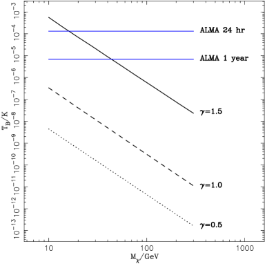
Figure 3: $M_{\chi}-T_{B}$ plane for three cusped dSph profiles, with an assumed NFW profile for the Milky Way (isothermal power-law models give almost identical results). We assume a 1” beam at 100GHz, and display the brightness temperature sensitivity for 24 hr and 1 yr ALMA observation.

However, we caution that the situation examined here may be over-simplified for the cusped models. If such density profiles really are followed to small radii, the Coulomb term neglected in Eq. 7 may become important. This effect requires a more thorough treatment to assess its impact – although extra cooling would lower the average electron energy, it would also drive the electrons closer to a thermal equilibrium. The spectral factor would in turn be closer to the thermal form, which tends to have larger values at the frequencies considered here. The CMB temperature shifts presented here may therefore be an underestimate at the cusp centre.

In addition, it is possible that the electron distribution may deviate from the dark matter cusp structure once the Coulomb term becomes dominant. In that case, the electron density distribution may become less steep, and more like a cored profile. On the one hand, this means that the peak signal will be lower. On the other, the signal averaged over a larger beam increases, as the effective cusp more closely matches the beam size. The tabulated temperature decrements increase with decreasing resolution precisely for this reason, and so a ‘smoother’ cusp is a better match to the angular scales of the telescopes mentioned above.

Table 4: List of $\bar{y}$ parameters for 1’ beam, fractional intensity shifts $\delta i$, and temperature decrements $\Delta T$ for both sets of dSph models. The remaining dSph parameters are as recorded in Table 3. We assume $M_{\chi}=10\mathrm{GeV}$ and $\langle\sigma V\rangle_{A}=10^{-26}\mathrm{cm^{3}s^{-1}}$. For the intensity and temperature shifts, we use a frequency of $x=0.616$ i.e. 35GHz.

$\gamma$	$\bar{y}/10^{-7}$	$\delta i/10^{-10}$	$\Delta T/10^{-9}$K
0.5	3.209 (3.208)	3.670 (3.590)	-2.731 (-2.671)
1.0	9.619 (9.582)	1.100$\times 10^{1}$ (1.096$\times 10^{1}$)	-8.186 (-8.155)
1.5	5.119$\times 10^{2}$ (5.499$\times 10^{2}$)	-5.854$\times 10^{2}$ (6.289$\times 10^{2}$)	-4.356$\times 10^{2}$ (-4.680$\times 10^{2}$)
$\alpha$	$\bar{y}/10^{-8}$	$\delta i/10^{-10}$	$\Delta T/10^{-10}$/K
0.2	4.399 (4.397)	5.031 (5.029)	-3.744 (-3.742)
0.0	4.473 (4.470)	5.115 (5.112)	-3.806 (-3.804)
-0.2	4.418 (4.414)	5.053 (5.048)	-3.760 (-3.757)

Table 5: The same as Table 4, but for a 1” beam.

$\gamma$	$\bar{y}/10^{-6}$	$\delta i/10^{-9}$	$\Delta T/10^{-9}$K
0.5	1.066 (1.057)	1.219 (1.209)	-9.075 (-8.999)
1.0	8.102$\times 10^{1}$ (7.251$\times 10^{1}$)	9.266$\times 10^{1}$ (8.292$\times 10^{1}$)	-6.895$\times 10^{2}$ (-6.171$\times 10^{2}$)
1.5	1.356$\times 10^{5}$ (1.466$\times 10^{5}$)	1.551$\times 10^{5}$ (1.677$\times 10^{5}$)	-1.154$\times 10^{6}$ (-1.248$\times 10^{6}$)
$\alpha$	$\bar{y}/10^{-8}$	$\delta i/10^{-11}$	$\Delta T/10^{-10}$/K
0.2	4.528 (4.471)	5.178 (5.113)	-3.853 (-3.805)
0.0	4.624 (4.548)	5.288 (5.201)	-3.935 (-3.871)
-0.2	4.599 (4.497)	5.259 (5.143)	-3.914 (-3.827)

Table 6: The same as Table 3, but for a 0.1” beam.

$\gamma$	$\bar{y}/10^{-6}$	$\delta i/10^{-9}$	$\Delta T/10^{-8}$K
0.5	1.636 (1.515)	1.871 (1.732)	-1.392 (-1.289)
1.0	1.544$\times 10^{3}$ (9.999$\times 10^{2}$)	1.766$\times 10^{3}$ (1.143$\times 10^{3}$)	-1.314$\times 10^{3}$ (-8.505$\times 10^{2}$)
1.5	7.893$\times 10^{6}$ (9.879$\times 10^{6}$)	9.026$\times 10^{6}$ (1.130$\times 10^{7}$)	-6.717$\times 10^{6}$ (-8.407$\times 10^{6}$)
$\alpha$	$\bar{y}/10^{-8}$	$\delta i/10^{-10}$	$\Delta T/10^{-10}$/K
0.2	5.200 (4.605)	5.946 (5.266)	-4.249 (-3.919)
0.0	5.440 (4.694)	6.221 (5.368)	-4.630 (-3.995)
-0.2	5.601 (4.665)	6.405 (5.335)	-4.767 (-3.970)

4.2 Upscattered Photons

We now consider explicitly the spectrum and flux of upscattered CMB photons, adopting the first-order, approximate approach described in Ensslin & Kaiser (2000).

4.2.1 Frequency Spectrum

The scattered spectrum of photons, $j\left(x\right)$, can be expressed as

$$j\left(x\right)=\int_{0}^{\infty}\mathrm{d}tP\left(t\right)i\left(x/t\right),$$ (41)

where the photon redistribution function $P\left(t\right)$ gives the probability of a photon being scattered to a frequency $t$ times greater than its original frequency. If the electron momentum spectrum is $f_{e}\left(p\right)\mathrm{d}p$, the photon redistribution function is

$$P\left(t\right)=\int_{0}^{\infty}\mathrm{d}pf_{e}\left(p\right)P\left(t;p\right).$$ (42)

In this expression, $P\left(t;p\right)$ is the redistribution function for a monoenergetic electron distribution. This has an analytic form

$$P\left(t;p\right)= -\frac{3|1-t|}{32p^{6}t}\bigl{[}1+\left(10+8p^{2}+4p^{4}\right)t+t^{2}\bigr{]}$$

$$+\frac{3\left(1+t\right)}{8p^{5}}\Bigl{[}\frac{3+3p^{2}+p^{4}}{\sqrt{1+p^{2}}}$$

$$-\frac{3+2p^{2}}{2p}\left(2\mathrm{arcsinh}\left(p\right)-|\ln\left(t\right)|\right)\Bigr{]},$$ (43)

with the condition that $P\left(t;\alpha,p_{1},p_{2}\right)=0$ if $|\ln\left(t\right)|>2\mathrm{arcsinh}\left(p_{2}\right)$. We may apply this formalism to the normalised electron momentum spectrum in Eq. (23). For such high electron energies, it is more convenient to express Eq (43) in terms of the logarithmic frequency shift $s=\mathrm{ln}\left(t\right)$, in which case:

$$P\left(s;p\right)=P\left(e^{s};p\right)e^{s}\mathrm{d}s.$$ (44)

$P\left(t\right)$ is plotted in Figure 4, for $M_{\chi}=10\mathrm{GeV}$ and $\langle\sigma V\rangle_{A}=10^{-26}\mathrm{cm^{3}\ s^{-1}}$ as before. Having computed this function, we calculate $j\left(x\right)$ via Eq. (41). In Fig.5, we plot $|j\left(x\right)-i\left(x\right)|$, which clearly displays the prominent emission in the radio and X-ray bands. The two regions are distinctly separated, with $i\left(x\right)$ constrained to radio frequencies, while $j\left(x\right)$ dominating in X-rays. There is virtually no overlap between the two. In addition, $j\left(x\right)$ peaks close to $x\sim 2.0\times 10^{5}$, corresponding to $p\sim 500$, as might be expected on the basis of the power-law nature of Eqn. (23), and the expected average electron momentum $p=4\gamma_{e}^{2}/3-1/3$.

4.2.2 X-ray Flux

The X-ray intensity produced by the upscattered photons can be calculated from Eq. (34). In this instance, we replace $\tilde{g}\left(x\right)\rightarrow j\left(x\right)$, and then the X-ray flux density is

$$F_{\rm Xray}\left(x\right)=I_{0}j\left(x\right)Y$$ (45)

where we integrate over the solid angle of the whole dSph.

We consider the X-ray emission integrated over a uniform efficiency energy band $0.1-10\mathrm{keV}$ (corresponding to $x_{1}=4.247\times 10^{5}$ and $x_{2}=4.247\times 10^{7}$), as an approximation to the current X-ray satellites Chandra and XMM-Newton. Dividing Eq. (45) by $x$ and integrating over the bandpass yields the X-ray photon flux

$$F_{\rm TOT}\left(x_{1},x_{2}\right)=\frac{I_{0}\tilde{Y}}{kT_{\rm CMB}}\int_{x_{1}}^{x_{2}}\frac{j\left(x\right)}{x}\mathrm{d}x.$$ (46)

For $M_{\chi}=10\ \mathrm{GeV}$ and $\langle\sigma V\rangle_{A}=10^{-26}\ \mathrm{cm^{3}\ s^{-1}}$, the integral above evaluates to

$$\int_{x_{1}}^{x_{2}}\frac{j\left(x\right)}{x}\mathrm{d}x=0.414.$$ (47)

The results for each of the models considered previously are listed in Table 7. The X-ray fluxes are all of order $10^{-12}\mathrm{cm^{-2}s^{-1}}$, above current estimates of the gamma-ray flux from direct annihilation channels, but well below what is currently possible to observe with X-ray satellites.

Table 7: List of integrated X-ray fluxes for Draco, in the energy band $0.1-10\mathrm{keV}$, for $M_{\chi}=10\ \mathrm{GeV}$ and $\langle\sigma V\rangle_{A}=10^{-26}\ \mathrm{cm^{3}\ s^{-1}}$.

$\gamma$	$F_{\rm TOT}/10^{-12}\mathrm{cm^{-2}s^{-1}}$
0.5	2.604 (2.564)
1.0	2.962 (2.914)
1.5	1.625$\times 10^{1}$ (1.795$\times 10^{1}$)
$\alpha$	$F_{\rm TOT}/10^{-12}\mathrm{cm^{-2}s^{-1}}$
0.2	1.325 (1.301)
0.0	1.539 (1.436)
-0.2	1.955 (1.654)

Figure 4: Photon redistribution function, for the momentum spectrum Eq. (24), assuming $M_{\chi}=10\ \mathrm{GeV}$.

Figure 5: $\log_{10}|j\left(x\right)-i\left(x\right)|$ against $\log_{10}\left(x\right)$, for the momentum spectrum Eq. (24). Note the two prominent bands, in the radio near $x\sim 2.5$ and in X-rays near $x=2.5\times 10^{5}$.

5 Conclusions

In the above analysis, we have shown the following:

• The Sunyaev-Zeldovich effect caused by secondary electrons produced from dark matter annihilation in dwarf galaxies (the dSZ effect) proposed by Colafrancesco (2004) could be measurable. The Comptonisation parameters averaged over the angular size of the dSph are $\bar{y}\sim 10^{-11}$ for low neutralino masses of $10\mathrm{GeV}$ and $\langle\sigma V\rangle_{A}=10^{-26}\mathrm{cm^{3}s^{-1}}$. The temperature decrement for an assumed beam size of $1^{\prime\prime}$ is of the order of milli-Kelvin for extremely cusped dSph halo models and a few tenths of a nano-Kelvin for cored models. This may provide a definitive test between these competing hypotheses, if the signal for cusped model is large enough to be detectable by future radio telescopes. This result holds before the noisy effects of primordial CMB, radio point sources, and SZ from clusters, has been taken into account. This, however, is only a concern for cored models, in which the signal comes from the bulk of the dSph. Even then, dSphs are clean and uncontaminated objects, devoid of magnetic fields and gas, and mostly free from point sources such as supernova remnants. For cusped models, most of the signal comes from the very centre and so contaminating point sources are not a worry.

• Our main aim here has been to demonstrate the feasibility of measuring the dSZ effect. We caution that our calculations make use of an approximate, single-scattering formalism that holds good for low electron optical depth. We may therefore have underestimated the size of the effect in the very innermost regions of cusped dSph models. Further numerical treatments, for example using the methods of Colafrancesco et al. (2003), in the vicinity of dark matter spikes are desirable.

• Upscattered CMB photons lie in the X-ray band, with the emission peak near $x=2.5\times 10^{5}$ for the neutralino mass considered here. Their integrated fluxes are $\sim 10^{-12}\ \mathrm{cm^{-2}\ s^{-1}}$, comparable in size to that from gamma-rays produced by direct annihilation channels. However, even next generation X-ray satellites such as Constellation-X, with collecting areas of $\sim 1000\mathrm{cm}^{-2}$ will struggle to detect such a signal.

• Our assessment of the importance of the dSZ effect is quite optimistic. If dark haloes are strongly cusped, then we conclude that the dSZ effect may be measurable in the near-future by telescopes like ALMA. However, if dark haloes are only weakly cusped, or if the dark matter particles are heavy ($\mathrel{\hbox to0.0pt{\lower 3.0pt\hbox{$\sim$}\hss}\raise 2.0pt\hbox{$>$}}50$ GeV), then even the most generous integration times with ALMA may not yield a positive detection. Nonetheless, it is worth bearing in mind that here are some circumstances in which a larger effect may be produced. First, the recently-discovered very dark dSph Ursa Major (Willman et al., 2005; Kleyna et al., 2005) may be the first representative of the missing dark satellites predicted by numerical simulations (Moore et al., 1998). In this case, there may be undetected, very dark dSphs much closer to us than Draco, which is beneficial as the flux received obviously varies like the inverse square of distance. Second, our calculations apply only to the case of the neutralino dark matter candidate. There are other possibilities, including light (1-5 MeV) scalar dark matter (Boehm et al., 2004; Hooper et al., 2004) and Kaluza-Klein dark matter (Bertone, Hooper & Silk, 2005), whose induced dSZ signals could well be of interest.

References

- Bertone, Hooper & Silk (2005) Bertone G., Hooper D., Silk J. 2005, Phys. Rep, 405, 279
- Binney & Tremaine (1987) Binney J., Tremaine S., 1987, Galactic Dynamics. Princeton University Press, Princeton
- Blasi & Colafrancesco (1999) Blasi P., Colafrancesco S. 1999, Astropart. Phys, 18, 649
- Boehm et al. (2004) Boehm C., Hooper D., Silk J., Casse M. 2004, PRL, 92, 1301
- Bonanos et al. (2004) Bonanos A.Z., Stanek K.Z., Szentgyorgi A.H., Sasselov D., Bakos G.A. 2004, AJ, 127, 861
- Bottino, Fornengo & Scopel (2003) Bottino A., Fornengo N. and Scopel S. 2003, PRD 67 063519
- Colafrancesco (2004) Colafrancesco S., 2004, AA, 422, L23
- Colafrancesco (2005) Colafrancesco S., 2005. In “IAU Colloquium 198: Near-Field Cosmology with Dwarf Elliptical Galaxies”, eds H. Jerhen, B. Bingelli, Cambridge University Press, in press
- Colafrancesco et al. (2003) Colafrancesco S., Marchegiani P., Palladino E., 2003, AA, 397, 27
- Colafrancesco & Mele (2001) Colafrancesco S., Mele B. 2001, ApJ, 562, 24
- Colafrancesco (2004) Colafrancesco S., 2004, AAP, 422, L23
- Diemand, Moore & Stadel (2004) Diemand J., Moore B., Stadel J., 2004, MNRAS, 353, 624
- Ensslin & Kaiser (2000) Ensslin T., Kaiser C. 2000, AA, 360, 417
- Evans (1994) Evans N. W., 1994, MNRAS, 267, 333
- Evans, Ferrer & Sarkar (2004) Evans N.W., Ferrer F., Sarkar S. 2004, PRD, 69, 123501
- Fomalont & Geldzahler (1979) Fomalont E.B., Geldzahler B.J. 1979, AJ, 84, 12
- Hill (1983) Hill, C.T., Nucl. Phys. B224, 469, 1983
- Hooper et al. (2004) Hooper D., Ferrer F., Boehm C., Silk J., Paul J., Evans N.W., Casse M., 2004, PRL, 93, 1302
- Jungman, Kamionkowski & Griest (1996) Jungman G., Kamionkowski M., Griest K. 1996, Phys. Rep, 267, 195
- Kamionkowksi & Turner (1991) Kamionkowski M., Turner M.S. 1991, PRD, 43, 1774
- Longair (1994) Longair M., High Energy Astrophysics, Cambridge University Press, Cambridge
- Moore et al. (1998) Moore B., Governato F., Quinn T., Stadel J., Lake G. 1998, ApJ, 499, L5
- Navarro, Frenk & White (1997) Navarro J., Frenk C.S., White S.D.M. 1997, ApJ, 490, 493
- Navarro et al (2004) Navarro J. F., Hayashi E., Power C., Jenkins A. R., Frenk, C. S., White S. D. M., Springel V., Stadel J., Quinn T. R., 2004, MNRAS, 349, 1039
- Kleyna et al. (2001) Kleyna J.T., Wilkinson M.I., Evans N.W., Gilmore G. 2001, ApJ, 563, L115
- Kleyna et al. (2005) Kleyna J.T., Wilkinson M.I., Evans N.W., Gilmore G. 2005, ApJL, in press (astro-ph/0507154)
- Raphaeli (1995) Raphaeli Y. 1995, ARAA, 33, 541
- Ruhl et al. (2004) Ruhl J.E., et al. 2004, Proc. SPIE., 5498, 11
- Tyler (2002) Tyler C. 2002, PRD, 66, 023509
- Willman et al. (2005) Willman B., et al. 2005, ApJL, in press (astro-ph/0503552)
- Wilkinson et al. (2004) Wilkinson M.I., Kleyna J.T., Evans N.W., Gilmore G., Irwin M.J., Grebel E.K. 2004, ApJ, 611, L21
- Zeldovich & Sunyaev (1969) Zeldovich Y.B., Sunyaev R.A., 1969, Ap&SS, 4, 301