Do extragalactic cosmic rays induce cycles in fossil diversity?

Abstract

Recent work has revealed a 62$\pm$3-million-year cycle in the fossil diversity in the past 542 My, however no plausible mechanism has been found. We propose that the cycle may be caused by modulation of cosmic ray (CR) flux by the Solar system vertical oscillation (64 My period) in the galaxy, the galactic north-south anisotropy of CR production in the galactic halo/wind/termination shock (due to the galactic motion toward the Virgo cluster), and the shielding by galactic magnetic fields. We revisit the mechanism of CR propagation and show that CR flux can vary by a factor of about 4.6 and reach a maximum at north-most displacement of the Sun. The very high statistical significance of (i) the phase agreement between Solar north-ward excursions and the diversity minima and (ii) the correlation of the magnitude of diversity drops with CR amplitudes through all cycles provide solid support for our model. Various observational predictions which can be used to confirm or falsify our hypothesis are presented.

1 Introduction

Rohde & Muller (2005) (hereafter RM) performed Fourier analysis of detrended data from Sepkoski’s compendium Sepkoski (2002) and found a very strong peak at a period of about 62 My. Monte Carlo simulations based on random walk models with permuted steps reveal a 99% probability that any such major spectral peak would not arise by chance, thus putting the diversity cyclicity on a firm statistical basis. The signal found by RM is robust against changes in procedure to improve aspects of uneven sampling and alternate methods of assessing significance Cornette (2007); Lieberman & Melott (2007). More recently Ding et al (2006) have identified a 61 My periodicity of lower significance in animal transmembrane gene duplication events, offset in phase about 2 radians from biodiversity; the peak in gene duplication events corresponds with the onset of the declining phase of biodiversity. Also, Rohde (2007) has noted the same sort of periodicity in ${}^{87}Sr$/${}^{86}Sr$ isotopic ratios, which is generally taken as a proxy for continental weathering rates. Cornette & Lieberman (2004) suggested a lack of significant long-term memory in the most of the fossil record, but they did not detrend nor examine lags beyond about 25 My. RM also argued that the five great mass-extinctions Raup & Sepkoski (1982) may be an aspect of this cycle. It is very interesting that the 62 My timescale is close to the current best value (63.6 My) for the period of the oscillation of the Sun in $z$, the distance perpendicular to the galactic disk Gies & Helsel (2005). The Sun is currently about 10 pc north of the plane, moving away, in an oscillation with amplitude about 70 pc. Finding a plausible mechanism tied to this vertical oscillation has been problematic. The primary reason is that midplane crossing (a possible time of enhanced interactions with galactic matter) would occur approximately every 32 My, which is not a spectral feature RM noted as significant in the diversity data. The same 32 My periodicity occurs if biological effects are strongest farthest from the galactic plane. A recently noted correlation between genus-level diversity and the amount of marine sedimentary rock outcropping has been taken as evidence that sampling bias may have led to the signal discussed here Smith & McGowan (2005). However, the extent and the lag between the timings genus diversity and rock outcrop curves and other factors suggest a common cause for these processes Peters (2005, 2006). Even if measured fossil biodiversity fluctuations are a consequence of the claimed periodic sampling bias, then a strong 62 My periodicity in rock outcropping would equally demand explanation. In general, the idea of astronomical forcings has been given a recent boost by a strong result showing rodent biodiversity fluctuations coupled to Milankovic cycles van Dam et al. (2006), with a similar periodicity noted for many clades elsewhere Martin & Meehan (2005). In what follows, we propose a possible explanation for this periodicity: enhanced cosmic rays when the solar system moves to the north side of the galactic plane.

2 Biodiversity and Cosmic Rays

Cosmic rays (CRs) may have many different strong biological and climatic effects. We do not advocate any particular mechanism for CR influence on the Earth biosphere. There are many such mechanisms which can impact fossil diversity, impacting species extinction and origination.

The first is direct radiation: CRs produce avalanches of secondary energetic particles Ferrari & Szuszkiewicz (2006), which are dangerous or lethal to some organisms. If the energy of the primary is below $10^{14}$ eV, only energetic muons can reach the Earth’s surface (some of the muons decays into electrons and positrons). Primaries with higher energies are able to produce air showers that reach the sea level and deliver energetic nucleons as well. (However, isotopes created by spallation typically have lifetimes of order 1 My or less, so that long-term oscillations in flux would be very difficult to detect.) Overall, secondary muons are responsible for about 85% of the total equivalent dose delivered by CRs. CR products account for $30-40\%$ of the annual dose from natural radiation in the US Alpen (1998). There is almost no protection from muons because of their very high penetrating depth, $\sim 2.5$ km in water or $\sim 900$ m in rock. Muons are known to produce mutations Micke et al. (1964). CRs are therefore a source of DNA damage causing mutations, cancer, etc. even for deep-sea and deep-earth organisms (Karam et al, 2001). It is beyond the scope of this paper to compute the absolute increase in the mutation rate. There are many causes of mutations. Generally, chemical mutagens induce point mutations, whereas ionizing radiation gives rise to large chromosomal abnormalities. Point mutations usually affect the operation of a single gene, but large-scale changes in chromosome structure can affect the functioning of numerous genes, resulting in major phenotypic consequences Lodish et al. (2000).

The second mechanism is climate change: There is good evidence that the ions produced by CRs in the atmosphere increase clouds Carslaw et al (2002); Marsh & Svensmark (2000); Svensmark et al. (2005); Harrison & Stephenson (2005); Shaviv (2005); Harrison & Stephenson (2006) which will increase planetary albedo. It has been argued that this can cool the climate. The global climate response should include changes in temperature and/or precipitation, but the amplitude is highly uncertain.

The effect of temperature on biodiversity is emprirically determined. The tropics have higher biodiversity, and recovery from mass extinctions is usually taken by repopulation from the tropics Jablonski et al. (2006). Furthermore, time series analysis of green algae, a particularly well-documented clade, shows correlation of biodiversity with global temperature over the last 350 My Aguirre & Riding (2005). Cool climates are usually drier, since evaporation from the ocean is reduced, and drought typically reduces biodiversity as well. So, the sign of the probable effect of increased cloud formation by CR is in agreement with the sign of biodiversity fluctuations. This is an area of active research; for example a new experiment startup at CERN (CLOUD) is designed to study the microphysics of cloud seeding by cosmic rays, and much more should be known in a few years.

The third mechanism is the mutagenic effect of oxides of nitrogen, NO_x (e.g. Cooney et al. (1993). CR ionization triggers lightning discharges Gurevich & Zybin (2005), which in turn affect the atmospheric chemistry (e.g., the ozone production by lightning and destruction by lightning-produced NO_x). CRs also increase the production of NO and NO₂ by direct ionization of molecules. Modifications in atmospheric chemistry by ionizing radiation, and the precipitation of NO_x as nitric acid can be numerically modeled Melott et al. (2005); Thomas et al. (2007). We plan to model this in detail based on the CR spectrum expected in our hypothesis.

The fourth mechanism is the mutagenic and damaging effect of solar UVB when the aforementioned NO_x damage the ozone shield. Both the indirect and direct production of these compounds catalyzes the depletion of ozone, making the atmosphere much more transparent to UVB (290-320 nm), which can cause mutations, cancer, and kill the phytoplankton which are at the the base of most of the marine food chain Melott et al. (2005). Terrestrial effects of variable CR flux have been discussed in the context of supernova explosions Erlykin & Wolfendale (2001); Gehrels et al. (2003) and the Sun’s motion in the local interstellar medium Zank & Frish (1999). These models produce random variations on time-scales of hundreds of thousands of years, so they cannot explain a much longer periodic signal. The idea of CR-diversity connection lies in line with the newly developed approach to mass extinctions as being produced by a combined effect of impulsive events and long-term stress called a “press” (Arens & West, 2006). Modulated flux of CR provides just such a long-term and periodic press.

One interesting possibility is the existince of multiple steady states when there exists a stronger continuous source of NO_x than exists in the present terrestrial atmosphere. There is a second steady state with an NO_x density several orders of magnitude higher than exists at present, which would have catastrophic effects not yet seen in simulations of astrophysical ionizations to date Kasting & Ackerman (1985). It will require substantial atmospheric ionization in the troposphere, probably coupled with an additional impulsive event to push the atmosphere toward the second attractor.

To summarize, a strong increase in CR flux may affect biodiversity by (1) direct radiation effects (mostly by muons) on the ground and in the seas down to perhaps 1 km, by (2) substantial climate change induced by cloud seeding of ionization, by (3) the chemical effects of atmospheric NO_x and its rainout as nitric acid, and by (4) increased solar UVB resulting from ozone depletion, a known effect of ionizing radiation on the atmosphere. It will require detailed research to quantify each of these effects.

3 Galactic Shock Model

Low-energy CRs with $10^{10}\textrm{ eV}\lesssim E\lesssim 10^{15}$ eV (below the “knee”) are thought to be produced by galactic sources: supernova explosions, supernova remnant shocks, pulsars Erlykin & Wolfendale (2001, 2005) (hence, referred to as galactic CRs), whereas higher-energy CR flux is dominated by particles accelerated in the galactic halo Fox et al. (2004) by the shocks in the galactic wind Williams et al. (2005a); Zirakashvili et al. (1996); Völk & Zirakashvili (2004) and at the termination shock Erlykin & Wolfendale (2005). (The boundary of $E\sim 10^{15}$ eV is imprecise: the galactic component likely extends to $\sim 10^{16}$ eV or even higher.) The galactic termination shock occurs when the fast, supersonic galactic wind interacts with the ambient intergalactic medium, much like the Solar wind termination shock on the outskirts of our Solar system Zank (1999). The position of the shock, which strongly depends on the properties of the “warm-hot intergalactic medium” Viel et al. (2005); Kravtsov et al. (2002); Williams et al. (2005b) (WHIM) and the wind speed, has been estimated Erlykin & Wolfendale (2005) to be $R\sim 100-200$ kpc for the wind speed $V\sim 300-500$ km/s. For these parameters with the Bohm diffusion coefficient, the extragalactic CR (EGCR) flux Jokipii & Morfill (1987) with $E<E_{c}\sim 10^{15}$ eV was expected to be attenuated by strong outward advection Völk & Zirakashvili (2004). However, the first measurement Kenney et al. (2005) of the wind speed yielded a much smaller value, $\sim 100$ km/s (less than the escape velocity from the galaxy, hence the outflow is called the “galactic fountain”). This puts the shock a factor of ten closer, hence decreasing the advection cutoff energy, $E_{c}$, by a factor of 30. Moreover, using a more realistic dependence of the diffusion coefficient on particle’s energy, $D\propto E^{s}$ with $s\simeq 0.3-0.6$ (for Bohm diffusion, $s=1$), yields the overall decrease of $E_{c}$ by a factor of $10^{3}$ to $10^{5}$. Thus, the galactic termination shock should be a natural source of EGCRs with energies as low as $\sim 10^{12}$ eV, i.e., those which produce muon showers in the Earth atmosphere. This EG component is, likely, subdominant at the present location of the Sun because of efficient shielding by galactic magnetic fields, but can be strong at large distances from the galactic plane, as we will show below. CR with energies around $10^{12}$ eV are the most dangerous to the Earth biota because they and their secondaries have the largest flux in the lower atmosphere: lower-energy ones are attenuated by the Earth magnetosphere, whereas the flux of the higher-energy particles rapidly decreases with energy.

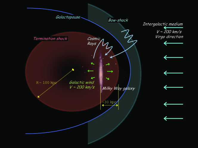
Figure 1: Cartoon representing the “galactosphere” with the galactic termination and bow shocks being sources of extragalactic cosmic rays. Due to inherent asymmetry, the north side of the Milky Way (with Virgo cluster being nearly at the north galactic pole) is exposed to a larger cosmic ray flux than its south side.

The global geometry of the “galactosphere” (by analogy with the heliosphere) is illustrated in Figure 1. The geometry of the termination and bow shocks causes the anisotropy of EGCRs around the Milky Way. In turn, the interaction of the gaseous envelope of the galaxy with the WHIM determines the shock geometry. The WHIM was formed by shock-heating in the early stages of cosmological structure formation and should pervade the connected large-scale structure predicted to form Melott et al. (1983) in the Cold Dark Matter scenario. Our galaxy moves at the speed of $\sim 150-200$ km/s toward the Virgo Cluster Williams et al. (2005b); Benjamin & Danly (1997), which is close to the galactic north pole.

The local WHIM is substantially pressure supported, thus having smaller infall velocity. Motion of the galaxy through the WHIM, at even moderate relative velocity, pushes the termination shock close to the north galactic face. Since the center of mass of the Local Group is at low galactic latitude, our galaxy should not be significantly shielded from interaction with with the WHIM pervading the Local Supercluster. The more moderate motion of the Solar system through the local interstellar medium, $\sim 23$ km/s (c.f., the Solar wind speed is $\sim 700$ km/s), produces strong asymmetry, with the shock distance in the “nose” and “tail” directions differing by more than a factor of two Zank (1999); Florinski et al. (2003). Therefore, the EGCR flux incident on the northern galactic hemisphere must be substantially larger than on the southern hemisphere. The predicted strong anisotropy CRs with $E\sim 10^{12}-10^{15}$ eV is outside the galaxy. At present Sun’s location — near the galactic plane — the magnetic shielding is very strong (as is discussed below), therefore the observed anisotropy should be very small and, likely, dominated by the (nearby) galactic sources. For higher-energy particles of energies about $10^{15}$ eV and above, our model agrees with previous studies, which predict that the CRs are not effectively trapped in the galactic wind; therefore the anisotropy is intrinsically small.

In order to see substantial periodic variation in the fossil record, the CR flux should have strong variation as well. We now demonstrate that the shielding effect provided by the galactic magnetic fields against EGCRs produces the required variation.

CRs with energies below the knee will propagate diffusively through the galaxy, e.g., in the vertical direction: from the north galactic face to the south, which results in (partial) shielding. A naive application of the standard diffusion approximation yields linear variation of the CR density as a function of $z$. Then the maximum variation of the EGCR flux on Earth would be $\sim\Delta/H\sim 5\%$, – too small to have strong impact on climate and biosphere [where $\Delta\simeq 70$ pc is the amplitude of the Sun vertical oscillation and $H\sim 1.5$ kpc is the exponential scale-height of the galactic disk region dominated by magnetic fields Beck (2001)]. This picture misses the fact that the magnetic field fluctuations in the galaxy are of high-amplitude Beck (2001), with $\delta B/\langle B\rangle\sim$few, and are likely Alfvénic in nature. Therefore, the effects of particle trapping and mirroring Narayan & Medvedev (2001); Malyshkin & Kulsrud (2002) are important.

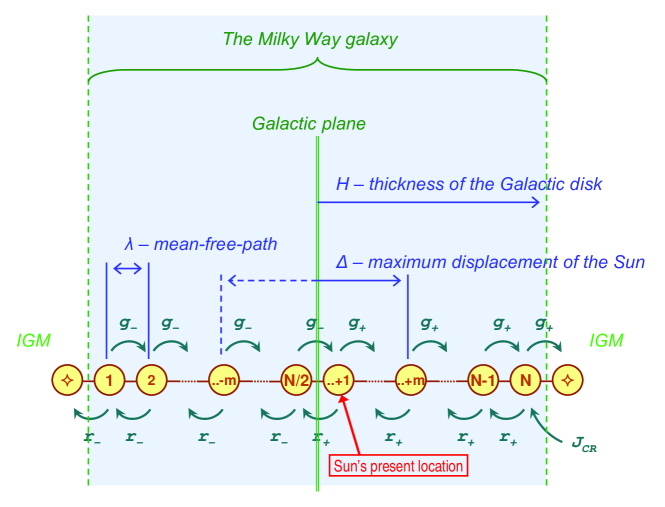
Figure 2: The galactic Markov chain. The cartoon represents the Markov chain model used to calculate Cosmic Ray diffusion through the Milky Way galaxy. The chain consists of $N$ normal sites and two absorbing ($*$) sites, which model particle escape. The transition probabilities are $r$ and $g$; their subscripts denote position: above ($+$) and below ($-$) the galactic plane. The in-flux of CRs is $J_{\rm CR}$. The Sun moves through sites between $N/2-m$ and $N/2+m$ and is presently located near the $N/2+1$ site.

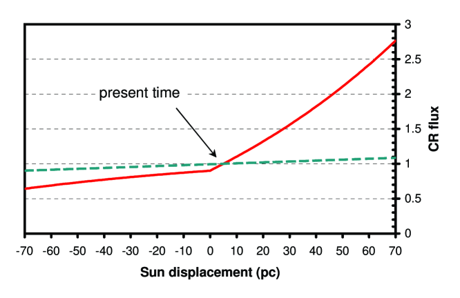
Figure 3: The extragalactic cosmic ray flux at the Earth relative to the present day value. The predicted EGCR flux (normalized to the present day value) in the Milky Way galaxy as a function of the distance from the galactic plane (in parsecs) for the asymmetric diffusion model (solid line). The standard diffusion model, predicting a 5% increase, is shown for comparison (dashed line). Clearly, a factor of five variation in the EGCR flux at the Earth is possible between south-most and north-most excursions of the Sun from the galactic plane. Here the flux variation, i.e., $F(70)/F(-70)$, is about 4.3. Since the Sun’s amplitude is a bit larger and varies, the overall max-over-min CR flux modulation amounts to about 4.6.

We know of no discussion of the effects of transient trapping and repeated mirroring in the presence of a mean field gradient (as in a galaxy) combined with random walk resulting in asymmetric diffusion, in which the probability of particle motion in forward and backward directions are unequal. This should not be confused with the standard diffusion, in which the probabilities are equal, though the diffusion coefficient can ce inhomogeneous and anisotropic, in general. The magnitude of the asymmetry is estimated in Appendix A. The number density of CRs in the galaxy is found using the one-dimensional Markov chain model shown in Figure 2. The galaxy is represented by $N$ sites, separated by one mean-free-path distance, thus $N\sim H/\lambda$. The two $*$-states at both ends are “absorbers” representing escape of CRs from the galaxy. The galactic plane is located half-way between $N/2$ and $N/2+1$ sites. The Sun moves through sites between $N/2-m$ and $N/2+m$, where $m\sim\Delta/\lambda$. At present, the Sun is at $z\simeq 8$ pc, which is around site $N/2+1$. The forward and backward transition probabilities are $r$ and $g$; their subscripts denote position: above ($+$) or below ($-$) the plane. There is in-flux of CRs, $J_{\rm CR}$, (produced at the termination shock in the northern hemisphere) through the right end. The observed CR flux decreases with energy roughly as $\propto E^{-3.1}$ above the knee and as $\propto E^{-2.7}$ at lower energies. We make a conjecture that the “true” EG flux has no break at $E\sim 3\times 10^{15}$ eV, whereas the observed break (the knee) is due to magnetic shielding discussed above. Thus, we conjecture that the EGCR flux outside the Galaxy exhibits no breaks up to $10^{12}$ eV, which could be a local maximum and which could smoothly join the lower energy calactic component. Thus, the EGCR flux of the most dangerous particles of $E\sim 10^{12}$ eV is about two orders of magnitude higher than the observed flux at this energy (though, it is still too small to affect the galactic structure, see more discussion in Appendix A). We use this value for the parameter $J_{\rm CR}$ of our model. An analytical solution for the CR density is plotted in Figure 3. An exponential increase of the local EGCR density with $z$ is seen. For contrast, we also plot the result of the standard diffusion model. Thus, very strong exponential shielding from EGCRs is found. Our estimates in of the CR flux are somewhat conservative in a number of places, so the actual flux may be a factor of few higher, and should depend on particle energy, the properties of the galactic magnetic fields and turbulence spectrum. Further details of CR propagation are included in Appendix A.

It should be understood that this solution contains only the CR variation due to solar motion normal to the galactic plane. There is an (unknown) additive component of CR due to, for example, supernovae. For example, there has apparently been a CR enhancement the last few My Lavielle et al. (1999), which is probably due to recent nearby supernovae, for which there is evidence for at least one about 2.8 Mya Knie et al. (2004), possibly associated with the formation of the Local Bubble in the interstellar medium Ma z-Apell niz (2001); Fuchs et al. (2006). The long-term variation we propose will be superimposed on these shorter-term variations.

4 Results

Figure 4 shows the detrended fossil genera fluctuation from Rohde & Muller (2005) and the computed EGCR flux from our model versus time for the last 542 My. The fossil data are timed to within the uncertainties of geological dating methods. Here we used the best available model data for the solar position $z$ versus time Gies & Helsel (2005) kindly provided to us by D. Gies. These calculations assume azimuthal symmetry of the Milky Way. The oscillation period and amplitude varies in response to the radial motion of the Sun and a higher density toward the Galactic center (included in the calculation) and a scatter from spiral arm passage (not included), see more discussion in Appendix C. Note that the long-term modulation of CR maxima in Figure 4 is real, being due to the Sun’s radial motion. Hence, one should also expect a weaker long-term cycle with a period $\sim 170$ My in the fossil record. The average period, accurate to about 7% Gies & Helsel (2005), $\sim 63.6$ My coincides precisely within uncertainty with the $62\pm 3$ My period of the fossil diversity cycle Rohde & Muller (2005). RM noted that the 62 My signal in the fossil record emerges from integration over almost 9 periods, and while highly significant does not coincide exactly with the onset of major extinction events, dated to within uncertainties in geological dating methods. These may be caused by a combination of stresses including for example CR flux variation, bolide impacts, volcanism, methane release, anoxia in the oceans, ionizing radiation bursts from other sources, etc. (It is an interesting aspect of this that the onset of the K/T (“dinosaur”) extinction, generally thought to be due to a bolide impact, coincides within 2 My of mid-plane crossing Gies & Helsel (2005).) Nevertheless, the 62 My cycle is strong and robust against alternate methods of Fourier decomposition and alternate approaches to computing its statistical significance (Lieberman & Melott, 2007).

A number of statistical tests have been performed in order to address the significance of the correlation between fossil data and modelled cosmic ray flux. In Appendices C and D, we discuss cross-correlation analyses involving the detrended data, the raw data for the short-lived genera [both samples are from Rohde & Muller (2005)], and Fourier-filtered samples. All tests show high statistical significance of the CR vs. diversity correlation. Namely, the detrended sample used by RM correlates with the CR flux from our model at the level of 49% (the Pearson coefficient is $r=-0.49$). The diversity data contains 167 discrete time periods; however only about 59% of the fossil data used is resolved to the bin size. For a conservative assessment of statistical significance, we take the effective number of bins as $\sim 167\times 0.59\approx 100$. The result is very high statistical significance that the observed correlation is not a consequence of coincidence (p-value $1.9\times 10^{-7}$). Consequently we conclude that the CR flux variation model may explain about one half of the long-term fluctuations in detrended biodiversity.

5 Discussion

The 62 My CR fluctuations are of course not the only source of diversity changes, but explain the long-period cycles quite well. Filtering out the short-term waves (the short-term component is largely dominated by the effect of the finite bin size of few My), the cross-correlation amplitude rises to $\sim 57$% at even higher better significance level (the probability of chance coincidence — p-value — is $6\times 10^{-10}$), see Appendix E for details.

Our model is predictive. An unavoidable consequence of the model is that the varying amplitude of solar excursions from the galactic plane modulates the CR flux and, consequently, affects the magnitude of the diversity drop. As we discussed above, variation in CRs are real in Figure 4. Thus, we look for possible correlation of the amplitude of the CR flux in each “cycle” and the amount of diversity drop (which we call “extinction strength”) in the corresponding diversity drop “event”. We applied an algorithm which finds for each CR cycle the local diversity minimum nearest to the CR maximum and the nearest preceding diversity maximum. The “extinction strength” is calculated as the difference between these maxima and minima. The CR amplitude is calculated analogously. Details are given in Appendix F.

The first result is that for each CR maximum there is always a diversity minimum within few My (the largest “mismatch” of 9 My is for the K/T extinction, which is likely due to a bolide impact). This is a strong result, given that some fossil bin sizes are as large as 5-6 My and, moreover, that only 59% of genera are resolved to this level. Second, Figure 5 shows an impressively strong correlation of the peak CR flux for each cycle in Figure 4 and the corresponding diversity drop. [Some uncertainty in the galactic structure data (magnetic fields, turbulence, halo structure) can affect the overall amplitude (normalization) of CR maxima, but not their rank order strengths.] A similar procedure was also applied to the raw data for short-lived genera to avoid biases in deep time due to the cubic fit. The results are shown in the Supplementary Information. The linear correlation coefficient of the CR flux amplitude and the extinction strengths shown in Figure 5 is over 93% and is significant, at the level of 99.93% (p-value of $6.8\times 10^{-4}$, computed from the Student distribution). This provides a very solid and independent confirmation of the model, which provides a natural mechanism for observed cycles in fossil diversity.

It should be noted that the cosmic ray enhancement axis shown in Figure 5 is a consequence of our assumed normalization of the EGCR flux. While our assumed flux is physically reasonable, other values are possible. Changing this assumption would stretch the CR axis, but would not change the rank order of the values nor modify their agreement with the diversity drop. Such a change would somewhat affect the shape of the CR curves in Figure 3, making a small change in the amplitude of the crosscorrelation. However, the agreement in period, phase, and rankorder diversity drops, the major pieces of evidence supporting our model, are not affected.

We emphasize that our hypothesis attempts to explain the very long term variations of the diversity and relate it to the long-term variation of the CR flux. We, by no means, attempt to explain every possible variation of the cosmic ray flux, which is known to be affected by galactic sources. For instance, a spiral arm crossing or a nearby supernova can substantially (depending on the distance) increase the CR flux at the Earth for the life-time of the supernova remnant, which is tens to hundreds of thousands years. Any such variation of CR flux may be “recorded”, e.g., in Earth isotope abundance, but has nothing to do with the discussed trend over hundreds of millions of years.

Our hypothesis is falsifiable. We predict that the termination and bow-shocks of our galaxy will be distributed sources of EGCR up to TeV energies at the galactic north, whereas only EGCR of $10^{15}$ eV will be reaching the Galaxy from it’s south. Such an anisotropy could potentially be observed directly (though shielding by and trapping in the galactic magnetic fields may diminish the effect substantially. A crude estimate yields about 1% anisotrophy, provided the effects of local CR sources is negligible. There are a number effects produced by CRs, some of which are evaluated in Appendix B, whereas others are postponed intil future publications. In particular, we predict that EGCR will upscatter 2.7 K cosmic microwave background radiation to the soft X-ray band ($\sim 200$ eV). The up-scattered flux shall constitute about $10^{-7}$ of the observed cosmic X-ray background. Similarly, EGCR will upscatter far and near infra-red (FIR and NIR) photons to about 10 keV and 1 MeV energies, respectively. The fraction of the upscattered photons compared to the hard X-ray and gamma-ray backgrounds is about $10^{-8}$ in both cases. Although the relative effects are rather weak, one can look for global north-south anisotrophy of cosmic X-ray and gamma-ray backgrounds. Averaging over half of the sky will substantially lower the statistical fluctuations of the backgrounds due to the galactic foreground emission. Taking the difference of the hemisphere-averaged signals may prove to be a useful strategy. Yet another possibility is to look for pion decay products (gamma-rays and neutrinos) produced in interactions of CR protons with neutral hydrogen in the Galaxy. We predict (see Appendix B) the emission of $\sim 2$ GeV protons with the flux of $\sim 1\%$ of the cosmic gamma-ray background at this energy. Detection of this excess emission from the northern Galactic hemisphere seems a feasible task for GLAST. Similarly, we predict the excess of $\sim 900$ MeV neutrinos with flux $\sim 3\times 10^{-4}\ {\rm particles/(m^{2}\ s\ sr)^{-1}}$, which may be a good target for IceCube.

To summarize, we have suggested that a substantial flux of cosmic rays is produced in a shock at galactic north, – a direction toward which our Galaxy has long been known to be moving in the Local Supercluster. We have shown that there is considerable shielding from the cosmic rays due to the gradient of both the regular and turbulent magnetic field in the Milky Way. When this is combined with the kinematics of the Sun in the Galaxy, based on its present motion and the galactic gravitational field, we find a highly statistically significant agreement between period, phase and relative magnitudes of excursions of extragalactic cosmic ray intensity and drops in biodiversity as measured by marine genera. There are many direct and indirect mechanisms by which cosmic rays may affect biodiversity. The cosmic ray periodicity discussed here accounts for about one-half of the biodiversity variance found by Rohde and Muller, and nearly all of their main feature, the 62 My oscillation. The model predicts that higher excursions of the Solar system above the galactic plane should produce more cosmic ray flux and larger biodiversity drops; this prediction is borne out by comparison between solar motion and paleontological data.

Appendix A Cosmic ray transport through the galaxy

CRs with energies below the knee in the galaxy propagate diffusively. The Larmor radii of the particles are smaller than the field inhomogeneities, so they nearly follow field lines. These fields are turbulent Havercorn et al. (2006); Beck (2001), hence the effective diffusion Chandran & Cowley (1998); Narayan & Medvedev (2001). One often assumes the Bohm diffusion coefficient for this process. As EGCR particles diffuse through the galaxy (in our case, in the vertical direction, from the north face to the south), their density decreases, thus resulting in shielding. As we pointed out in the text, a naive application of the diffusion approximation yields linear variation of the CR density with $z$ of about 5%, for typical galactic parameters Beck (2001)). High-amplitude magnetic field fluctuations in the galaxy Beck (2001) affect diffusion via mirroring and transient trapping effects Narayan & Medvedev (2001). In the presence of the mean field gradient, they modify diffusion so that it becomes asymmetric (not to be confused with anisotropic diffusion, where diffusion is still symmetric, but the rates depend on position and orientation). We are not aware of discussion of this effect in the literature.

In asymmetric diffusion, the probabilities of the forward and backward transitions are not equal. To estimate the magnitude of the asymmetry, recall that the amplitude of turbulent magnetic fluctuations is maximum on large spatial scales and decreases as magnetic energy cascades to small scales. Hence trapping by large-amplitude waves occurs on scales comparable to the field correlation length Havercorn et al. (2006), hence $\lambda\sim 20$ pc. (The mean-free-path, $\lambda$, depends on particle’s energy as well.) Trapping is intermittent and transient because large-amplitude, quasi-coherent Alfvénic wave-forms (“magnetic traps” or “magnetic bottles”) exist for the Alfvén time. Thus, a trapped CR particle, moving at almost the speed of light, experiences about $N_{b}\sim c/V_{A}\sim 3\times 10^{3}$ bounces (for the interstellar medium field $B\sim 3~{}\mu$G and density $\rho\sim 3\times 10^{-26}$ g/cm³, where $V_{A}=B/\sqrt{4\pi\rho}$ is the Alfvén speed) during the bottle lifetime. Reflection conditions are determined by the particle loss-cones on both ends of the magnetic bottle. There is a field gradient ($B$ decreasing away from the galactic plane on a distance $\sim H$. The precise value of $H$ not known, but it does not significantly affect the results of our model). The loss-cone conditions imply that, on average, more particles are reflected from a higher-field end (closer to the galactic plane) than from the lower-field one. From the loss-cone condition, we estimate the reflected fraction in one bounce as $\epsilon_{0}\sim\lambda[\langle B\rangle/(\nabla\langle B\rangle)]\sim 10^{-2}$. Since particles also interact with the smaller-amplitude, high-frequency background of short-scale Alfvén waves, the particle distribution function evolves toward isotropization while trapped particles traverse the magnetic bottle. We assume some 1% efficiency of this process, $\eta\sim 0.01$. This leads to a small “leakage” of particles from the trap, predominantly in the direction away from the galactic plane. The total “leaked out” fraction per the trap lifetime is $\epsilon\sim 1-(1-\eta\epsilon_{0})^{N_{b}}$. The efficiency depends on the numerous factors, such as the level of Alfvénic small-scale turbulence which induce pitch-angle scattering of CRs in and out of the loss cones, the relative phase-space volumes occupied by the loss cones and the trapped regions, the in- and outgoing fluxes of CRs relative to the local density of particles at a given Markov site. The latter depend upon the total leaked out faction of particles, thus $\eta$ should be determined self-consistently via numerical modeling. A complete calculation of all these processes will be presented elsewhere.

The number density of CRs in the galaxy is found using the one-dimensional Markov chain model shown in Figure 2 and discussed in the text. Note that the forward and and backward transition probabilities above and below the galactic plane are $r_{+}=g_{-},\ r_{-}=g_{+}$, by symmetry. Their ratio is $g_{+}/r_{+}\sim 1+\epsilon$, with $\epsilon$ obtained in the previous paragraph. An analytical solution for the CR density is plotted in Figure 3. An exponential increase of the local EGCR density with $z$ is seen. There, the result of the standard diffusion model, i.e., with $\epsilon=0$ is also shown. Very strong exponential shielding effect is seen (the EGCR flux at low energies is normalized by the present day value to unity).

The amplitude of the EGCR flux variation is determined by the total EG flux outside the galaxy and the structure of magnetic fields and turbulence inside the galaxy. The flux of EGCRs outside the Milky Way can readily be evaluated, taking into account that the effective shielding scale-height is about few hundred pc (a factor of few smaller than $H$) because at about 100 pc away from the galactic plane, the galactic wind is beginning to form (c.f., the thickness of the thin galactic disc is $\sim 80$ pc). This wind stretches the magnetic fields in the $z$-direction (wind direction), thus dramatically increasing the field correlation length and the particle mean-free-path, $\lambda$, and decreasing the turbulence level of small-scale Alfvénic fluctuations responsible for pitch-angle diffusion. These both effects reduce the exponential suppression nearly to the standard diffusion value above $z\sim 300$ pc or so. This extrapolation yields that the EGCR flux outside the Milky Way is about one hundred times larger than the local value.

The CR flux above the knee (above $10^{15}$ eV) is thought to be primarily extragalactic in origin (these CRs are not trapped in the galaxy because of their large Larmor radii), and it decreases with energy roughly as $\propto E^{-3.1}$. Below the knee, the CR spectrum is shallower, namely $\propto E^{-2.7}$, whereas the CR particles are “trapped” in the galactic magnetic fields. We make a conjecture that the “true” EG flux has no break at $E\sim 3\times 10^{15}$ eV, whereas the observed break (the knee) is due to magnetic shielding discussed above. Thus, the EGCR flux of the most dangerous particles of $E\sim 10^{12}$ eV is about two orders of magnitude higher than the observed flux at this energy. This value of the EGCR flux matches nicely the extrapolated value of the CR flux discussed in the previous paragraph (as well as with the overall energetics of the galactic wind).

Here we also comment that such high EGCR flux is still too low to affect the global galactic structure (via CR pressure). The CR pressure in the galaxy is dominated by particles with energies below tens of MeV per nucleon (the Earth is protected from them by the Solar Wind) and constitutes up to ten percent of the total pressure. However, we discuss here the much more energetic particles, with energies above ten TeV, which are not attenuated by the Solar Wind and the Earth magnetic fields. With the galactic CR spectrum $\propto E^{-2.7}$ at low energies, one obtains that these dangerous TeV EGCRs contribute less than 0.1% of the total pressure. This is an upper limit on the EGCR pressure outside the Milky Way. Inside the galaxy, the EGCR pressure is lower because of magnetic shielding. Hence it has no influence on the dynamics of the interstellar medium and the galactic structure while having a potentially devastating effect on life on the Earth.

The assumed EGCR flux at and above TeV is reasonable on energetic grounds. Indeed, the kinetic energy density in the outflowing galactic wind is of order the energy density of galactic CRs Erlykin & Wolfendale (2005). Some fraction, $\eta$, of the wind energy goes into acceleration of EGCR at the galactic termination shock. Thus, one can estimate, by analogy with the previous paragraph, that the lower limit on the conversion efficiency is about $\eta>10^{-3}$. This is a very reasonable value, given large uncertainties in the galactic halo structure, its magnetic fields, the diffusion coefficient and its dependence on particle energy, etc.

Our estimates in of the CR flux are somewhat conservative in a number of places, so the actual flux may be a factor of few higher. We also neglected here that the CR flux at Earth depends on the injected energy spectrum at the termination shock and on the particle mean-free-path in the galactic fields, which is energy-dependent. Thus, the amplitude of CR fluctuations should depend on particle energy, the properties of the galactic magnetic fields and turbulence spectrum.

Appendix B Observational predictions of the model

The large anisotropy of EGCR could potentially be detected. Since we are now well inside the galaxy and shielding is very strong, direct detection of CR north-south anisotropy is complicated. The expected anisotropy at the present location of the Earth can cruedly be estimated from the model parameter $J_{CR}$, the fraction of CR entering the Galaxy from the north that leave it at the south. This yelds the anisotropy being of order 1%. However, this does not take into account any (local) galaxtic sources of CR that can “contaminate” the signal. Studies of CR anisotropies indicate their existence at 0.1%-1% level. However, they are mostly attributed to the local magnetic field structure — spiral arms. This is reasonable because charged particles propagate nearly freely along field lines (mostly parallel to the galactic plane) and diffuse across them in the vertical direction. Recent Milagro, Super-Kamiokande and Tibet Air Shower Array results indicate the presence of the anisotropy at the level of 0.1% in the Galactic center direction and along the Galactic north-south direction (Atkins, et al., 2005; Oyama, 2006; Amenomori, et al., 2006). However, the absence of the Compton-Getting effect may imply that the galaxy-wide anisotropy could be smeared out by a propagation effect through the co-moving local interstellar medium.

One can think of some indirect methods. For instance, TeV EGCR can Compton up-scatter CMB photons to energies of $\sim\gamma^{2}(2.7{\rm K})\sim 200~{}{\rm eV}$. The up-scattered flux of photons is of order $F_{scatt}\sim F_{CMB}\tau$, where the optical depth to scattering is $\tau\sim R\sigma_{p\gamma}(4\pi F_{CR}/c)$, where in turn $F_{CR}$ is the EGCR flux outside the Galaxy, $R$ is the typical size of the system being of order the distance to the shock, and $\sigma_{p\gamma}\sim 0.1$ mb is the typical $p-\gamma$ cross-section. With the conjectured CR flux $F_{CR}\sim 10\ ({\rm m^{2}\ s\ sr})^{-1}$ at 1 TeV and $R\sim 30$ kpc, we obtain the upscattered flux of order $\sim 2\times 10^{-2}\ ({\rm m^{2}\ s\ sr})^{-1}$. The galactic north-south anisotropy of these soft X-ray photons could be a clear signature of our model. However, detection of such anisotropy can be difficult because of large contamination by gas line emission at these energies and strong hydrogen absorption of these soft X-rays. Indeed, the cosmic soft X-ray background (CXB) is about $\sim 10^{5}\ ({\rm m^{2}\ s\ sr})^{-1}$ at 0.5–1 keV (Hickox & Markevich, 2005). This yields that the upscattered photon flux is about $10^{-7}$ of the CXB, which makes it hard to observe.

TeV cosmic rays can also up-scatter infrared (IR) photons. Cosmic IR background has two peaks, in the far and near infrared, at approximately $\sim 10^{-2}$ eV and 1 eV. Up-scattering of FIR and NIR photons brings them to about 10 keV and 1 MeV, respectively. The FIR and NIR fluxes at the peaks are approximately $2\times 10^{-8}$ and $3\times 10^{-8}$ ${\rm W\ m^{-2}\ s^{-1}\ sr^{-1}}$. The up-scattered fluxes are calculated to be of order $4\times 10^{-5}$ and $4\times 10^{-7}\ {\rm photons\ m^{-2}\ s^{-1}\ sr^{-1}}$. The ratio of the up-scattered fluxes to the hard X-ray (at 10 keV) and gamma-ray (at 1 MeV) background fluxes (Hickox & Markevich, 2005; Miniati, et al., 2007) are about $10^{-8}$ in both cases.

Yet another possibility is to look for $\gamma$-rays at GeV energies due to interaction of TeV EGCRs with the interstellar gas in molecular clouds and production of pions, which then produce $\gamma$-rays via decay ($\pi^{0}$’s are of great interest because their motion is not affected by the galactic magnetic fields). The $p-p$ cross-section for neutral (and charged) pions is rougly $\sigma_{pp}\sim 30$ mb (Dermer, 1986) for proton center of mass energies of $\sim 30$ GeV, which corresponsd to interaction of TeV CRs with neutral hydrogen in the Galaxy. For the estimate, we assume the neutral hydrogen column density $N_{H}\sim 10^{21}$ cm^-2 (this is somewhat higher than the average column density toward the Galactic poles). The collisional depth is $\tau\sim N_{H}\sigma_{pp}\sim 3\times 10^{-5}$. This yields the gamma-ray flux of about $F_{\gamma}\sim 3\times 10^{-4}\ ({\rm m^{2}\ s\ sr})^{-1}$. Neutral pions decay $\pi^{0}\to 2\gamma$ to produce $\sim 70$ MeV photons (in the center of mass frame). Thus, we predict emission of gamma-rays of energy of $\sim 2$ GeV from pion decay. The ratio of the predicted gamma-ray flux to the cosmic gamma-ray background (Miniati, et al., 2007) is of order 1%, which seems feasible to detect. Such an observation would be an interesting task for GLAST. This effect will be addressed in a subsequent publication.

Similarly, interaction of TeV CRs with neutral hydrogen produces charged pions, which decay into muon neutrinos of energy $\sim 900$ MeV. Similar estimates yield neutrino flux of about $F_{\nu}\sim 3\times 10^{-4}\ {\rm particles/(m^{2}\ s\ sr)}^{-1}$ at $0.9$ GeV. These neutrinos can be observed with IceCube.

Appendix C Model of the solar motion through the Milky Way

The solar motion through the Milky Way has been computed for the past 600 My and kindly provided to us by D. Gies Gies & Helsel (2005). A number of axisymmetric galaxy models have been presented and analyzed by Dehnen & Binney (1998a). Gies’ computation uses the best model of the global density distribution in the galaxy, according to the analysis of that paper Dehnen & Binney (1998a). The density normalization Dehnen & Binney used is about $0.17~{}M_{\odot}~{}\textrm{pc}^{-3}$, which is somewhat higher than the local density of $0.1\pm 0.01~{}M_{\odot}~{}\textrm{pc}^{-3}$ found by these authors Dehnen & Binney (1998b) and other groups Holmberg & Flynn (2000, 2004); Bienayme et al (2006) from the Hipparcos parallax data. The latter, low value of the galactic density results in a longer period of vertical oscillations at the present position of the Sun, as long as $82\pm 2$ My, which is substantially larger than the average period of 64 My. It should be noted, however, that Hipparcos has determined parallaxes and distances to stars within 200 pc (in the galactic plane) around the Sun. Even with the very low Sun velocity with respect to the local rest frame, $v\sim 13$ km/s (c.f., nearby stars have typical velocities of about $\sim 40$ km/s), the Sun will traverse the Hipparcos-probed region within 15 My, much shorter than 64 My average period. The low local density is consistent with the fact that the Sun is in the inter-arm region at present. The strength of the spiral arms is still debated Amaral & Lepine (1997), however recent Doppler measurement of a maser in the Perseus arm Binney (2006) indicates very strong contrast of the arm—inter-arm density. With a reasonable 50% duty cycle (the Sun arm-crossing time vs. inter-arm residence time) the average oscillation period is in agreement with 64 My.

Dehnen & Binney (1998a) used Hipparcos data in their models. However, instead of using the local galactic density as a normalization, they considered it as a free (fit) parameter, which they found by fitting observables, e.g., the star terminal velocities Feast & Whitelock (1997). These are, in turn, determined from proper motions found by Hipparcos. Since such measurements do not depend on parallax distances, one probes distances as large as 3 kpc. Thus, such a technique is much more accurate to constrain a global galactic model. Of course, the axisymmetric model misses the local density inhomogeneities (e.g., due to spiral arms), which should result in some scatter of the Sun oscillation period. In fact, the diversity period does show a larger scatter than the computed vertical oscillation (and the related CR flux).

Appendix D Statistical analysis

The correlation between two data sets is evaluated with the Pearson moment correlation coefficient, $r$, a dimensionless index that ranges from –1.0 to 1.0 inclusive and reflects the extent of a linear relationship between the two sets. For two sets of $N$ values each, $X$ and $Y$, the r-value is calculated as

$$r=\frac{N\left(\Sigma\,XY\right)-\left(\Sigma\,X\right)\left(\Sigma\,Y\right)}{\sqrt{\left[N\left(\Sigma\,X^{2}\right)-\left(\Sigma\,X\right)^{2}\right]\left[N\left(\Sigma\,Y^{2}\right)-\left(\Sigma\,Y\right)^{2}\right]}}.$$ (D1)

The statistical significance of the correlation is evaluated from the Student t-distribution. The t-distribution is used in the hypothesis testing of sample data sets and gives the probability (p-value) of the chance coincidence. In the limit of large number of degrees of freedom (data points), it approaches the Gaussian distribution. For non-zero $r$,

$$t=\sqrt{{r^{2}(N-2)}/{(1-r^{2})}}$$ (D2)

obeys the Student’s t-statistics with $N-2$ degrees of freedom.

Appendix E Correlation of CR flux and diversity data

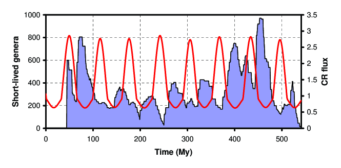
Figure 6: The short-lived genera variation and extragalactic cosmic ray flux at the Earth calculated from our model. The short-lived genera (blue curve, left scale) as a function of time over-plotted with the normalized cosmic ray flux calculated from our model (red curve, right scale). Note that the most of the minima in genera number nearly coincide with cosmic ray maxima, as in Figure 4.

All the diversity data used in our analysis are taken from supplementary information files of Rohde & Muller (2005) paper. The cross-correlation of the predicted CR flux and the de-trended diversity data is discussed in the text. One can worry that the de-trending strongly affects the data and can introduce biases. In their original paper, RM demonstrated that the 62 My periodic signal is seen even in the raw data. In order to emphasize the effect, they separated all genera into two categories: short-lived (with the first and last occurrence dates being separated by 45 My or less) and long-lived. Only short genera shows the periodic variation, although with less statistical significance than the de-trended data. The raw short-lived genera data overlaid with the CR flux is shown in Figure 6. The cross-correlation coefficients and the statistical significances for both data sets are given in Table 1. Clearly, both data show correlation at very high statistical significance.

Spectral analysis by Fourier Transform builds on the result that almost any mathematical function can be decomposed into a sum of sinusoids. The RM cyclicity result does not imply that the diversity record is sinusoidal, but that it does contain one or more components around 62 My in period which are anomalously large. Our model would explain the basis of this large component; our cross-correlation result implies that the model can explain about half the overall variance in the fossil record.

Our model would predict the long-term variation of diversity, with a period of about 64 My. The data, however, contains all time-scales. The Fourier harmonic spectrum shown in RM contains, in addition to the two cycles, a long tail of short-frequency harmonics. This short-frequency component is largely dominated by data binning, which sizes vary from 1 My to 9 My, and contaminate the data set. Therefore, we performed a separate statistical analysis of the data, in which short-time variations are filtered out. We applied three different filtering techniques to the de-trended data from RM paper. A low-pass filter performs a forward Fourier transform to calculate the spectrum, sets all Fourier harmonics with frequencies greater than 1/(35 My) to zero and then performs the inverse Fourier transform to restore the signal. A narrow window filter uses the same technique, but now keeps harmonics only within a narrow window around the 62 My peak. The weighted window filter is analogous to the narrow window one, but now the diversity spectrum is weighted with (multiplied by) the normalized spectrum of the Solar motion, $z(t)$, which does show a prominent harmonic peak around 63 My. The correlation coefficients and the statistical significance levels are given in Table 1. Overall, data filtering increases the correlation substantially; the statistical significance rises to nearly 100%. All these results confirm that our CR model describes the long-term variation of diversity very well. Note that for the weighted window filter technique, the filtered data contains certain information on $z(t)$ and hence on the CR flux. These two data sets — the CR flux and the filtered data — are not statistically independent, therefore we do not evaluate the statistical significance of the correlation.

It is also interesting to cross-correlate our CR model with the origination and extinction data sets separately. RM’s Fourier analysis of these sets shows that neither yields as strong a 62 My-signal as the combined diversity data. They argued, therefore, that the cycle is likely due to a combination of effects, rather than just the extinction or just the diversification alone. Our study confirms this conclusion. The correlations of CR flux with the origination intensity and with the extinction intensity from RM data are very weak and statistically insignificant (p-value is greater than 0.2 in both cases). These results are also summarized in Table 1. One must note, however, that if either had a phase offset with respect to biodiversity, cross-correlation would be weak. Lieberman & Melott (2007) have investigated this further.

Appendix F Correlation of diversity drops and CR maxima

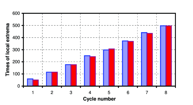
Figure 7: Diversity minima coincide with CR maxima. The bar-chart shows the times of CR maxima, second column in Table 2, (red bars) and the times of the nearest local minima of diversity, fourth column in Table 2, (blue bars) versus the cycle number. The times of diversity minima are uncertain to few My due to large sizes of data bins (about 5 My, typically).

Our model predicts that a higher CR flux should result in a larger diversity drop. To check whether this prediction is confirmed by the available data, we used the following algorithm. First, one finds all local maxima of the CR flux through the entire domain of 542 My. The times at which the CR flux is at maximum in each cycle and the corresponding value of the flux amplitude of variation, calculated as the difference of the values at maximum and the preceeding minimum, are given in columns two and three in Table 2. Application of the same algorithm to the de-trended data yields inaccurate results, because subtraction of the cubic fit introduces a large number of spurious local minima (the whole curve becomes saw-tooth-like, as is seen from Figures in RM and our Figure 4). A much more accurate way to find local extrema is to use the short-lived data instead. Since the cubic fit describes the global trend on the time-scale of 500 My, its subtraction hardly affects the local structure and we can use these $T_{min}$ and $T_{max}$ for further analysis of both de-trended and short-lived genera sets. Thus, in the next step, for each CR $T_{max}$ one finds the nearest local minimum and the nearest preceding local maximum in the diversity curve. These values are given in columns four and five in Table 2. For all extrema, except just one, the data has the resolution coarser than 1 My (often 3-5 My). For such large data bins, one takes the median value of $T$ for the bin. It is interesting that each CR peak has a so-defined diversity drop within the cycle (not a single cycle is missed). Moreover, the CR maxima and diversity minima nearly coincide, within few My. The CR maxima times and the diversity minima times are shown in Figure 7 versus the cycle number. The correspondence of the minima/maxima is remarkable.

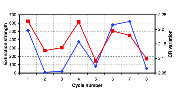
Figure 8: The extinction strength of short-lived genera and extragalactic cosmic ray peak strength versus the cycle number. As in Figure 4, the extinction strength (blue curve, left scale), calculated as the diversity drop from each cycle from preceding peak to minimum, and the relative EGCR intensity at maximum from our model (red curve, right scale) are plotted versus the cycle number (numbering is backward from the present).

The drop in diversity, which we refer to as “extinction strength”, is defined as the difference in genera diversity at the maximum and the minimum, that is at times $T_{max}$ and $T_{min}$ given in columns 4 and 5 of Table 2. The extinction strengths are calculated for both data sets, i.e., for the de-trended genera and the short-lived genera. They are given in the last two columns of Table 2. They are also plotted in Figures 5 and 8. The correlation in both cases is very strong. Although the short-lived genera set is not the “main” sample — neither in RM paper, nor in the present study, — it is remarkable that both samples show such strong correlations. Thus, it justifies that the found correlations are real. The correlation analysis shows, in particular, that CR maxima are correlated with diversity drops with $r=0.80$ and $p=0.017$ (that is, 80% correlation at 98.3% confidence level) for the short-lived genera set, and with $r=0.93$ and $p=0.0007$ (that is, 93% correlation at 99.93% level, meaning that there is less than 0.07% probability of the data-points happened to become “aligned” this way by chance) for the de-trended data.

Table 1: Correlation data of the cosmic ray flux and various diversity data sets. The first group of data set are data from Rohde & Muller (2005). The second group represents de-trended data filtered with the low-pass filter (to isolate long-term variations), the narrow window and the $z(t)$-weighted window function (to isolate harmonics close to the 62 My cycle). In the latter case, the statistical significance and the p-value are not evaluated because the data sets (filtered and CR) are not independent. The third group includes the origination and extinction data from the supplementary information of Rohde & Muller (2005).

data set	cross-correl. (r-value)	stat. significance	p-value
de-trended data	– 0.49	$\sim$ 100%	$1.9\times 10^{-7}$
short-lived genera	– 0.32	$\sim$ 99.9%	$1.1\times 10^{-3}$
long-lived genera	0.11	$\sim$ 70%	0.29
low-pass filter	– 0.57	$\sim$100%	$6.4\times 10^{-10}$
narrow window	– 0.72	$\sim$100%	$2.0\times 10^{-17}$
weighted window	– 0.74	—	—
origination intens.	– 0.0039	3%	0.97
extinction intens.	– 0.067	44%	0.56

Table 2: Diversity drops and CR maxima. The columns are: (1) cycle number, (2) time at which CR flux is at maximum, (3) maximum value of the CR flux, (4) time of the local diversity minimum closest to CR $T_{max}$, (5) time of the closest preceding local maximum of diversity, (6) extinction strength calculated from the de-trended data, (7) extinction strength calculated from the short-lived genera data.

Cycle       #	CR:       $T_{max}$	CR-flux             variation	Divers.: $T_{min}$	Divers.: $T_{max}$	Extinc.:         de-trend.	Extinc.: short-lived
1	50 My	2.23	59 My	74 My	704	512
2	115 My	2.13	115 My	121 My	50	10
3	176 My	2.14	177 My	184 My	37	22
4	242 My	2.26	250 My	273 My	700	376
5	306 My	2.09	298 My	308 My	61	82
6	368 My	2.19	372 My	400 My	572	579
7	434 My	2.18	441 My	454 My	616	621
8	496 My	2.10	497 My	501 My	94	55

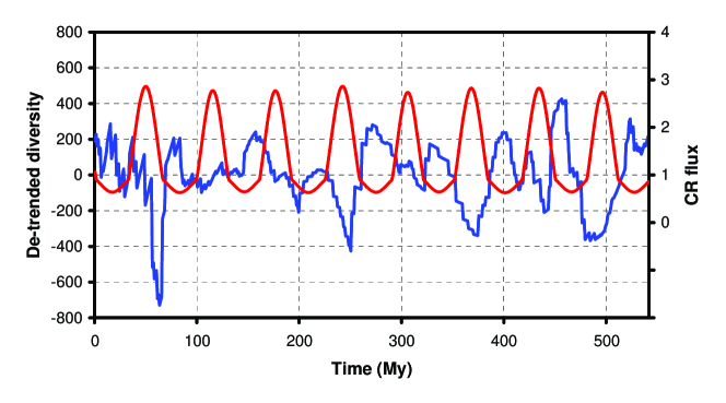
Figure 4: The diversity variation (from Rohde & Muller, 2005) and extragalactic cosmic ray flux at the Earth calculated from our model. The de-trended diversity variation (blue curve, left scale) as a function of time over-plotted with the normalized cosmic ray flux calculated from our model (red curve, right scale). There are no fit (and free) parameters in the model. The maxima in the cosmic ray flux coincide with minima of the diversity cycle. Note also that the onset times of the diversity decline coincide with moments of the rapid increase of the flux.

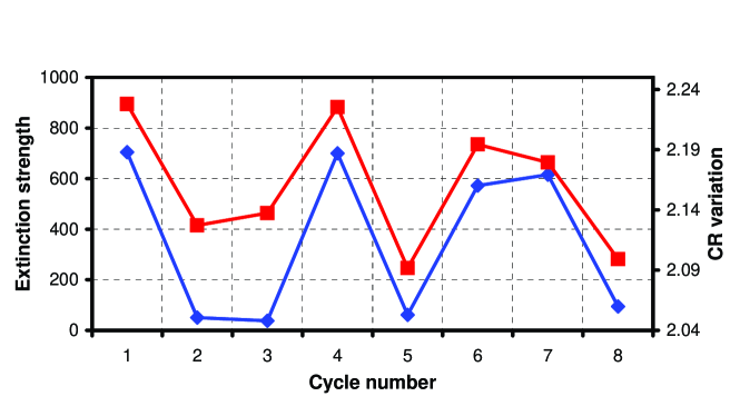
Figure 5: The correlation of the extinction strength and the amplitude of the extragalactic cosmic ray flux. The extinction strength (blue curve, left scale), calculated in each cyclic “event” in Figure 4 as the diversity drop from the preceding local maximum to the local minimum, and the amplitude of the EGCR intensity variation from our model (red curve, right scale) are plotted versus the cycle number (numbering is backward from the present). The correlation is about 93% and has a probability less than one part in a thousand of arising from chance.

References

- Aguirre & Riding (2005) Aguirre, J., & Riding, R. 2005, Palaios 20, 581
- Alpen (1998) Alpen, E.L. 1998, Radiation Biophysics (San Diego: Academic Press)
- Amaral & Lepine (1997) Amaral, L.H., & Lepine, J.R.D. 1997, MNRAS, 286, 885
- Amenomori, et al. (2006) Amonomori, et al. 2006, Science, 314, 439
- Arens & West (2006) Arens, N.C., & West, I.D. 2006, GSA annual meeting abstract 230-1
- Atkins, et al. (2005) Atkins, R., et al. 2005, astro-ph/0502303
- Beck (2001) Beck, R. 2001, Space Sci. Rev., 99, 243
- Benjamin & Danly (1997) Benjamin, R.A. & Danly, L. 1997, ApJ, 481, 764
- Bienayme et al (2006) Bienayme, O. et al. 2006, A&A, 446, 933
- Binney (2006) Binney, J.J. 2006, Science, 311, 44
- Carslaw et al (2002) Carslaw, K.S., Harrison, R. G., & Kirkby, J. 2002, Science, 298, 1732
- Cornette (2007) Cornette, J.L. 2007, Computer Science Engineering, in press.
- Cornette & Lieberman (2004) Cornette, J.L. & Lieberman, B.S. 2004, Proc. Natl. Acad. Sci., 101, 187
- Chandran & Cowley (1998) Chandran, B.D.G. & Cowley, S. 1998, Phys. Rev. Lett., 80, 3077
- Cooney et al. (1993) Cooney, R.V. et al. 1993, Proc. Nat. Acad. Sci. (USA) 90, 1771
- Dehnen & Binney (1998a) Dehnen, W. & Binney, J.J. 1998a, MNRAS, 294, 429
- Dehnen & Binney (1998b) Dehnen, W. & Binney, J.J. 1998b, MNRAS, 298, 387
- Dermer (1986) Dermer, C. D. 1986, ApJ, 307, 47
- Ding et al (2006) Ding, G. et al. 2006, PLOS Computational Biology, 2, 0918.
- Erlykin & Wolfendale (2001) Erlykin, A.D. & Wolfendale, A.W. 2001, J. Phys. G: Nucl. Part. Phys., 27, 959
- Erlykin & Wolfendale (2005) Erlykin, A.D. & Wolfendale, A.W. 2005, J. Phys. G: Nucl. Part. Phys., 31, 1475
- Feast & Whitelock (1997) Feast, M. & Whitelock, P. 1997, MNRAS, 291, 683
- Ferrari & Szuszkiewicz (2006) Ferrari, F. & Szuszkiewicz, E. 2006, astro-ph/0601158
- Florinski et al. (2003) Florinski, V., Zank, G. P., & Axford, W. I. 2003, Geophys. Res. Lett., 30, 5
- Fox et al. (2004) Fox, A.J., Savage, B.D., Wakker, B.P., Richter, P., Sembach, K,R., & Tripp, T.M. 2004, ApJ, 602, 738
- Fuchs et al. (2006) Fuchs, B. et al. 2006 MNRAS, 373, 993
- Gehrels et al. (2003) Gehrels, N. et al. 2003 ApJ, 585, 1169
- Gies & Helsel (2005) Gies, D.R. & Helsel, J.W. 2005, ApJ, 626, 844
- Gurevich & Zybin (2005) Gurevich, A.V. & Zybin, K.P. 2005, Phys. Today, 58, 37
- Harrison & Stephenson (2005) Harrison, R.G. & Stephenson, D.B. 2005, Proc. R. Soc. A. doi:10.1098/rspa.2005.1628
- Harrison & Stephenson (2006) Harrison, R.G. & Stephenson, D.B. 2006, Proc. R. Soc.: Math., Phys. & Enginer. Sci., 462, 1471
- Havercorn et al. (2006) Haverkorn, M., et al. 2006, ApJ, 637, L33
- Hickox & Markevich (2005) Hickox, R. & Markevich, M. 2005, ApJ, 645, 95
- Holmberg & Flynn (2000) Holmberg, J. & Flynn, C. 2000, MNRAS, 313, 209
- Holmberg & Flynn (2004) Holmberg, J. & Flynn, C. 2004, MNRAS, 352, 440
- Jablonski et al. (2006) Jablonski, D., Roy, K., & Valentine, J.W. 2006, Science 314, 102
- Jokipii & Morfill (1987) Jokipii, J.R., & Morfill, G. 1986, ApJ, 312, 170
- Karam et al (2001) Karam, P.A., Leslie, S. A., & Anbar, A. 2001, Health Physics, 81, 545
- Kasting & Ackerman (1985) Kasting, J.R., & Ackerman, T.P. 1985, J. Atmo. chem. 3, 321
- Kenney et al. (2005) Keeney, B.A., Danforth, C.W., Stocke, J.T., Penton, S.V., & Shull, J.M. 2005, submittted to the proceedings of IAU colloquium No. 199, “Probing galaxies through quasar absorption lines,” (Eds. Williams, R.P., Shu, C., Menard, B.)
- Knie et al. (2004) Knie, K. et al. 2004 Phys. Rev. Lett. 93, 171103
- Kravtsov et al. (2002) Kravtsov, A.V., Klypin, A.A., & Hoffman, Y. 2002, ApJ, 571, 563
- Lavielle et al. (1999) Lavielle, B. et al. 1999, Earth Planet. Sci. Lett. 170, 93
- Lieberman & Melott (2007) Lieberman, B.A, & Melott, A.L. 2007, in preparation.
- Lodish et al. (2000) Lodish, H. et al 2000, Molecular Cell Biology, (W.H. Freeman: New York)
- Malyshkin & Kulsrud (2002) Malyshkin, L. & Kulsrud, R. 2002, ApJ, 549 402
- Ma z-Apell niz (2001) Ma z-Apell niz, J. 2001 ApJ, 560, L83
- Marsh & Svensmark (2000) Marsh, N.D. & Svensmark, H. 2000, Phys. Rev. Lett., 85, 5004
- Martin & Meehan (2005) Martin, L.D. & Meehan, T.J. 2005, Naturwissenschaften 92, 1
- Melott et al. (1983) Melott, A.L., et al. 1983, Phys. Rev. Lett., 51, 935
- Melott et al. (2005) Melott, A.L. et al. 2005, Geophys. Res. Lett. 32, L14808 doi:10.1029/2005GL023073
- Micke et al. (1964) Micke, A. et al. 1964, Proc. Nat. Acad. Sci. (USA) 52, 219
- Miniati, et al. (2007) Miniati, F., Koushiappas, S., Di Matteo, T. 2007, astro-ph/0702083
- Narayan & Medvedev (2001) Narayan, R. & Medvedev, M.V. 2001, ApJ, 562, 129
- Oyama (2006) Oyama, Y. 2006, astro-ph/0605020
- Peters (2005) Peters, S.E. 2005, Proc. Natl. Acad. Sci., 102, 12326
- Peters (2006) Peters, S.E. 2006 Paleobiology 32, 387
- Raup & Sepkoski (1982) Raup, D. & Sepkoski, J. 1982, Science, 215, 1501
- Rohde (2007) Rohde, R.A. 2007, GSA Abstract 63-7
- Rohde & Muller (2005) Rohde, R.A. & Muller, R.A. 2005, Nature, 434, 208
- Sepkoski (2002) Sepkoski, J., 2002 Bull. Am. Paleontol., no. 363, (eds. Jablonski, D. & Foote, M., Paleontological Research Institution, Ithaca)
- Shaviv (2005) Shaviv, N.J. 2005, J. Geophys. Res., A8, A08105
- Smith & McGowan (2005) Smith, A.B. & McGowan A.J. 2005, Biology Lett., 1, 443
- Svensmark et al. (2005) Svensmark, H., et al. 2005, AGU Fall meeting abstract, 52B, 06
- Thomas et al. (2007) Thomas, B.c., Jackman, C.H., & Melott, A.L. 2007 Geophys. Res. Lett., accepted (http://arxiv.org/abs/astro-ph/0612660)
- van Dam et al. (2006) van Dam, J.A. et al. 2006, Nature, 443, 687
- Viel et al. (2005) Viel, M., et al. 2005, MNRAS, 360, 1110
- Völk & Zirakashvili (2004) Völk, H.J. & Zirakashvili, V.N. 2004, A&A, 417, 807
- Williams et al. (2005a) Williams, R.J., Mathur, S., & Nikastra, F. 2005a, astro-ph/0511621
- Williams et al. (2005b) Williams, R.J., Mathur, S., & Nikastro, F. 2005a, astro-ph/0512003
- Zank (1999) Zank, G.P. 1999, Space Sci. Rev., 89, 413
- Zank & Frish (1999) Zank, G.P. & Frisch, P.C. 1999, ApJ, 518, 965
- Zirakashvili et al. (1996) Zirakashvili,V.N., Breitschwerdt, D., Ptuskin, V.S., & Völk, H.J. 1996, A&A, 311, 113