Comprehensive Analysis of RXTE Data from Cyg X-1: Spectral Index-Quasi-Periodic Oscillation Frequency-Luminosity Correlations

Abstract

We present timing and spectral analysis of $\sim$ 2.2 Ms of Rossi X-ray Time Explorer (RXTE) archival data from Cyg X-1. Using a generic Comptonization model we reveal that the spectrum of Cyg X-1 consists of three components: a thermal seed photon spectrum, a Comptonized part of the seed photon spectrum and the iron line. We find a strong correlation between the 0.1-20 Hz frequencies of quasiperiodic oscillations (QPOs) and the spectral index. Presence of two spectral phases (states) are clearly seen in the data when the spectral indices saturate at low and high values of QPO frequencies. This saturation effect was discovered earlier in a number of black hole candidate (BHC) sources and now we strongly confirm this phenomenon in Cyg X-1. In the soft state this index-QPO frequency correlation shows a saturation of the photon index $\Gamma\sim 2.1$ at high values of the low frequency $\nu_{L}$. The saturation level of $\Gamma\sim 2.1$ is the lowest value found yet in BHCs. The bolometric luminosity does not show clear correlation with the index. We also show that Fe K_α emission line strength (equivalent width, EW) correlates with the QPO frequency. The EW increases from 200 eV in the low/hard state to 1.5 keV in the high/soft state. The observational correlations revealed compel us to propose a scenario for the spectral transition and iron line formation which occur in BHC sources. We also present the spectral state (power-law index) evolution for eight years of Cyg X-1 observations by RXTE.

1 Introduction

Cyg X-1 is one of the brightest high-energy sources in the sky, with an average 1-200 keV energy flux of $\sim 3\times 10^{-8}$ ergs cm^-2s^-1. Its optical companion is an O9.7 Iab supergiant HDE 226868. Estimates of the mass, M, of the X-ray star, $5{{}_{<}\atop{}^{\sim}}M_{\odot}{{}_{<}\atop{}^{\sim}}15$ [e.g., Herrero et al. (1995)] strongly suggest the presence of a black hole. Observed spectral and temporal X-ray characteristics are extensively studied based on the large amount of data collected in the RXTE archive (see §2 for the data description). Our analysis includes $\sim$ 2.2 Ms of Rossi X-ray Time Explorer (RXTE) archival data from Cyg X-1 to study the spectral and timing properties of this classical BHC source.

One of the basic questions addressed in many observational and theoretical studies concerning relativistic compact objects is how to observationally distinguish between a neutron star (NS) and a black hole (BH). Cyg X-1, being extensively studied, has often been used as the prototypical example of a BH. The different patterns, for example correlations between spectral and timing characteristics of BH and NS sources, has been proposed as a criteria for determination of the nature of the compact object. Recently Belloni (2005) and McClintock & Remillard (2004) published a concise review of the observational features of the spectral states in BH sources where they also point out a link between timing and spectral properties of X-ray radiation and plasma ejection leading to radio jets.

Titarchuk, & Fiorito (2004), hereafter TF04, and Titarchuk & Shaposhnikov (2005), hereafter TSh05, present theoretical and observational arguments how to distinguish between BH and NS binaries. TF04 present observational evidence that in BHs two distinct phases occur: one of them, the steep power-law phase (so “called” high/soft state), is the signature of a BH. In the soft state of BH the spectral index-quasiperiodic oscillation (QPO) frequency correlation shows a flattening, or “saturation” of the photon index $\Gamma$ at high values of the low frequency $\nu_{L}$. This saturation effect was identified as a BH signature. TSh05 demonstrate that this saturation is not present in at least one NS source. They show that for 4U 1728-34 the index $\Gamma$ increases monotonically with $\nu_{L}$ . We show here that Cyg X-1 is a perfect example of a BH source as the suggested BH index-QPO frequency correlation is observed with clear features of the saturation at high and low frequencies.

Long-term monitoring of Cyg X-1 has revealed two distinct spectral states and transitions between them [see a review of Cyg X-1 early observations in Zhang et al. (1997)]. Simultaneous, low- and high energy X-ray observations during interstate transitions have been obtained by several groups in 1996 [see references in Zhang et al. (1997) and Cui et al. (1997, 1998)]. In the low/hard state, the power-law portion of the spectrum is relatively flat with a photon index $\Gamma$ of about 1.5. They found that a majority of the time Cyg X-1 stayed in the low/hard with an occasional transition (during their observations, duty cycle of this state was about 90 %) to the soft state where the power-law spectrum became significantly steeper (with $\Gamma\sim 2.5$). Also, one or two times per year Cyg X-1 exhibited so called ”failed state transitons”, when it started to transition but did not reach a soft state, stopping at some intermediate state and their falling back. Thus one can claim that the source was predominantly in a hard state in 90s. However Wilms et al. (2005) have recently shown that since 2000 the source spent $\sim 34\%$ of the time in the intermediate and the soft state. We came to the same conclusion as a result of our analysis of the source spectral transition (see more discussion of this phenomenon in §4, the last paragraph).

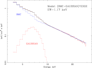
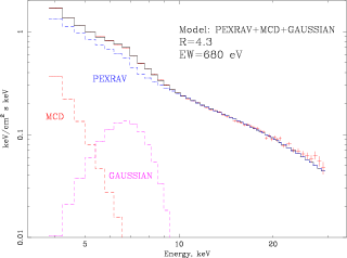
Figure 1: Comparative fits with BMC and PEXRAV models for the observation during the high/soft state.

As Cui et al. (1997) pointed out there is strong evidence that the observed QPO characteristics are related to spectral properties: the QPO amplitude increases as the energy spectrum becomes harder. They also discovered QPO low-frequencies varying in the range of 4-10 Hz during the spectral transition. In fact, using these observations Di Matteo & Psaltis (1999), hereafter DP99, found that the photon index can be correlated with the QPO frequency. One can see a few points of this correlation in the frequency range from 1 to 10 Hz in their Figure 1. This behavior was later confirmed by Pottschmidt et al. (2003), hereafter P03, using observations of the Cyg X-1 spectral transition in 2000-2001. It is worth noting that DP99 also suggested that the index-qpo frequency correlation can be a common phenomenon for black hole sources.

In this Paper we present a detailed study of spectral transitions in Cyg X-1 and demonstrate how the energy spectra are related to the power density spectra (PDSs), in particular the QPO features. We find that the index-QPO correlation is similar to previous findings for BH sources, e.g. DP99, Vignarca et al. (2003) and TF04, where the QPO frequency-index correlation is presented for large samples of BH sources. In PDSs observed by RXTE for Cyg X-1, we show that these QPO low frequencies tightly correlate with the break frequency $\nu_{b}$.

Titarchuk, & Osherovich (1999) presented a model for the radial oscillations and diffusion in the transition layer (TL) surrounding the BH and NS. Using dimensional analysis, they identified the corresponding radial oscillation and diffusion frequencies in the TL with the low-Lorentzian $\nu_{L}$ and break frequencies $\nu_{b}$ for 4U 1728-34. They predicted values for $\nu_{b}$ related to the diffusion in the transition layer, that are consistent with the observed $\nu_{b}$. Both the Keplerian and radial oscillations, along with diffusion in the transition layer, are controlled by the same parameter: the Reynolds number $\gamma$ (inverse of $\alpha$-viscosity parameter), which in turn is related to the accretion rate [see also Titarchuk, Lapidus & Muslimov (1998), hereafter TLM98]. It is worth noting that the identification of the break frequency as a diffusion effect (the inverse of time of the diffusion propagation in the bounded configuration) was later corroborated by both Wood et al. (2001) and Gilfanov & Aref’ev (2005). Particularly, Wood et al. demonstrated that the black hole candidate (BHC) XTE 1118+480 X-ray light curves with fast rise/exponential decay profile are a consequence of the diffusion matter propagation in the disk. On the other hand, Gilfanov & Arefiev (2005) studied X-ray variability of persistent LMXBs in the $\sim 10^{-8}-10^{-1}$ Hz frequency range aiming to detect PDS features associated with the diffusion time scale of the accretion disk $t_{diff}$. As this is the longest intrinsic time scale of the disk, the power spectrum is expected to be independent of the frequency below $\nu_{b}~{}(<1/t_{diff})$. They found that the break frequency correlates very well with the binary orbital frequency in a broad range of binary periods from $P_{orb}\sim 12$ min to 33.5 days, in accord with theoretical expectations for the diffusion time scale of the disk.

Zhang et al. (1997) found while the low-energy X-ray (1.3-12 keV) and high-energy X-ray (20-200 keV) fluxes strongly anticorrelate during the spectral transition, the bolometric luminosity in the soft states may only be 50%-70% greater than the hard state luminosity. On the other hand, Frontera et al. (2001) found that the increase of the bolometric flux in the high/soft state with respect to that in the low/hard state is about s factor of $3$. In this Paper we further explore this issue of the bolometric luminosity using the data collected from the PCA and HEXTE detectors of RXTE. In fact, we confirm Zhang’s et al. finding that the bolometric luminosity slightly increases when Cyg X-1 undergoes transition from the low/hard to the soft states. We also comment on the issue of how the wind in Cyg X-1 affects the bolometric luminosity.

Petterson (1978) and Kaper (1998) argue that the X-ray source in Cyg X-1 is powered mainly by accretion from the strong stellar wind of the supergiant star. Cyg X-1 probably represents a situation intermediate between pure, spherical wind accretion and accretion by Roche lobe overflow. As Gies et al. (2003) pointed out the density of the wind determines the size of X-ray ionization zone surrounding the black hole. This in turn controls the acceleration of the wind in the direction of the black hole. During the low/hard state, the strong wind is fast and accretion rate is relatively low, while during the soft state, the weaker, ionized wind attains only a moderate velocity and the accretion rate increases. It is evident that the Thomson optical depth of the wind increases in spectral transition because of decrease of the wind velocity (even if outflow mass rate is constant through the state transition). We further investigate the effects of the wind in Cyg X-1 in terms of power and energy spectra, bolometric luminosities and the strength of K_α iron line emission.

The iron line observed in Cyg X-1 is the strongest among the Galactic black holes. Barr et al. (1985) discovered the broad Fe K_α line, with equivalent width $EW=120$ eV and FWHM=1.2 keV in an EXOSAT spectrum of Cyg X-1. Because of these features are broad one should be concerned that the profiles are artifacts of inadequate continuum models or instrumental effects. Miller et al. (2002) argue that an Fe K_α line is required to obtain statistically acceptable fits to spectra observed from Cyg X-1 with a number of instruments, for a variety of continuum models and source luminosities [see Ebisawa et al. (1996), and Cui et al. (1998) for ASCA results, and see Di Salvo et al. (2001) and Frontera et al. (2001) for BeppoSAX results]. It is important to emphasize that most of the observations indicate that the relatively strong broad Fe K_α line emission which EW is within a range of 100-300 eV while Miller et al. claim their best-fit model for Chandra spectrum includes a broad line ($E\sim 5.8$ keV, FWHM$\sim 1.9$ keV, $EW=170\pm 70$ eV) component along with a narrow Gaussian emission line ($E\sim 6.4$ keV, FWHM$\sim 80$ eV, $EW=16\pm 3$ eV) component. It is clear that the inferred values of line energy E, FWHM and EW are affected by the energy resolution of a given instrument and by the continuum model applied [see e.g. Frontera et al. (2001)]. Recently Miller & Homan (2005) revealed a strong and broad Fe K_α line in another black hole source, GRS 1915+105 ($EW\sim 150-360$ eV). They suggest that there should be a link between EWs and QPO frequencies in BH sources. Here we show that indeed there are correlations between the strength of the iron line, QPO frequency and the spectral index.

The observational signature of the mass accretion rate $\dot{M}$ is the QPO low frequency as it has been shown for BH sources by TF04. The QPO frequency is related not only to $\dot{M}$ but also to the size of the Comptonizing region, $R$, i.e. $\nu_{QPO}\propto 1/R$. The behavior of $\nu_{QPO}$ with respect to spectral index $\Gamma$ connects the characteristics of the Comptonization and spectral state with $\dot{M}$. This is graphically represented for BHs in the observations of Vignarca et al. (2003). We similarly employ this type of analysis to compare Cyg X-1 spectral states with other BHs to show their qualitative differences.

In §2 we present the details of the our spectral and timing data analysis of archival RXTE data from the BH source Cyg X-1. In §3 we present and discuss the results of the data analysis and we compare them to that presented by TF04 for other BH sources. In §3 we also offer an explanation various correlations found in Cyg X-1. Discussion and conclusions follow in §4.

2 Observations and data analysis

For our analysis we used data from Proportional Counter Array (PCA) and High-Energy X-ray Timing Experiment (HEXTE) onboard RXTE. The data is available through the GSFC public archive . Cyg X-1 is one of the sources most extensively observed by RXTE. We searched the entire archive for public data. The summary of the RXTE observation proposals and data used in the present analysis, and a reference to the corresponding proposal IDs, are given in Table 1. Each proposal consists of a set observations that can be divided into intervals of continuous on-source exposure (usually about 3 ks) corresponding to one RXTE orbit. For each proposal we provide its archival identification number (proposal ID), the dates between which the data were collected, the total on-source exposure, the number of continuous data intervals $N_{int}$, the average number of operational PCUs in the proposal ${\bar{N}_{PCUon}}$. The data spans $\sim 8$ years of data with almost 2.2 Ms of the total on-source exposure. We calculated an energy spectrum and an averaged PDS for each continuous interval of data, which correspond to one orbital RXTE revolution. Data reduction and analysis was conducted with FTOOLS 5.3 software according to recipes in the “RXTE Cook Book”.

2.1 Timing Analysis

Before being transmitted to ground-based station the PCA data is preprocessed by six event analyzers, two of which are always operating in Standard1 and Standard2 modes. To avoid telemetry overload for very bright sources such as Cyg X-1 the counts from several energy ranges are processed by separate on-board event analyzers and stored in separate data files. During most observations, Binned mode with several millisecond time resolution combining counts from 0 to 35 PCA energy channels is available. Depending on RXTE epoch, this channel range corresponds to energy range changing from 1.5-10 keV to 2.0-15 keV. We were mostly interested in low frequency range ($\leq$ 100 Hz) and the temporal resolution of this mode is sufficient for our analysis. Otherwise, we used sub-millisecond resolution Event or Single Bit Mode data. The data was rebinned to a $2^{-11}$ second time resolution to obtain a Nyquist frequency of 1024 Hz. PDSs are normalized to give rms fractional variability per Hz. For the PDS modeling we used the broken power law (see van Straaten et al., 2000, for definition) component to fit broad band frequency noise and Lorentzians to describe QPO profiles.

2.2 Spectral Analysis

Spectral data reduction and modeling was performed using the XSPEC astrophysical fitting package. First we performed the data screening to calculate good time intervals for Fourier analysis. We excluded the data collected for elevation angles less than $15^{\circ}$ and during South Atlantic Anomaly passage. To avoid the electron contamination we also applied the condition for electron rate in the PCU 2 (which is operational during all observations) to be less than 0.1 counts/sec. We extract energy spectra from Standard2 data files using counts from upper xenon layer of all operational detectors. Then we applied a deadtime correction to account for detector dwell time after each event detection. Current response matrices for PCA and HEXTE give 10%-20% offset for relative cross-normalization. Henceforth, when we fit PCA and HEXTE spectra simultaneously, we multiply the physical model applied to the data by a constant factor to account for this instrumental discrepancy. We fix the factor value at unity for PCA data set while allowing it to change for the HEXTE Cluster A and B spectra. In Table 2 we give the values of the best fit model parameters along with the offset values obtained for representative PCA/HEXTE spectrum for each source state.

To describe the continuum spectrum we use the Bulk Motion Comptonization (BMC) model which is a generic Comptonization model. This model can be used if the photon energy is less than the mean electron energy of the Compton cloud $E_{av}$. The choice of a particular theoretical model is provided by robust nature of the BMC model for different spectral states and independence of a specific type of Comptonization scenario involved. The BMC model spectrum is a sum of the blackbody component (which is the disk radiation directly seen by the observer) and the fraction of the blackbody component Comptonized in the corona with the variable Comptonization fraction. The model has four parameters: $kT$ is a color temperature of thermal photon spectrum, $\alpha$ is the energy spectral index ($\alpha=\Gamma-1$, where $\Gamma$ is the photon index), the parameter $A$ is related to the weight of the Comptonized component, $A/(1+A)$, and a normalization of the blackbody component. The BMC model is valid for the general case of Comptonization when both bulk and thermal motion are included.

For the thermal Comptonization $E_{av}$ is related to electron temperature $E_{av}\sim kT_{e}$. When the bulk motion Comptonization is dominant $E_{av}$ is related to the bulk kinetic energy of the electrons $E_{av}{{}_{<}\atop{}^{\sim}}m_{e}c^{2}$. For the thermal Comptonization for energies less than $E_{av}$ CompTT and BMC models are identical. The thermal Comptonization and dynamical (bulk motion) Comptonization are presumably responsible for the spectral formation in the hard state and the soft state respectively. Therefore, one needs a generic model such as BMC that describes the spectral shape regardless of the specific type of Comptonization. Although the thermal Comptonization model can properly fit the spectral shape for the observed spectra for all spectral states but it would give physically unreasonable values of the best-fit parameters for the soft state spectra. Notably, Wilms et al. (2005) show optical depth of Compton Cloud inferred from CompTT model significantly decreases towards high/soft state. It is very difficult (in the framework of any reasonable physical model) to explain tendency when the mass accretion rate increases during the hard-to-soft state transition.

We remind a reader that TSh05 used two BMC components to fit the spectral data from NS source 4U 1728-34. The radiation from the central object and inner parts of accretion disk is Comptonized by a surrounding cloud. As long as the spectral index for each BMC component is a physical characteristic of the Comptonizing region, TSh05 used this parameter for each of BMC components describing disk and NS Comptonized radiation. In fact, the BMC XSPEC model spectrum (Titarchuk et al. 1997) is a sum of the (disk or NS) black-body component and Comptonized black-body component. In the BH case one can conclude that only one the BMC component is needed in order to describe the Comptonization spectrum. The soft photons generated by the solid surface are absent in this case.

Another important issue in modeling the BHC spectra is a proper account for iron fluorescence line at $\sim 6.4$ keV. As it was already mentioned, the iron line observed in Cyg X-1 is one of the strongest among BHC sources and is confirmed by various instruments. The site of the iron line origin is not yet identified and the process of its formation is under debate. Currently it is fashionable to explain the iron line in the framework of the reflection model by Magdziarz & Zdziarski (1995) (hereafter MZ95, see PEXRAV and PEXRIV models in XSPEC). The geometry required by the model implies that the source of Comptonized component (exponentially cut-off power law) is located above a flat reflecting surface (accretion disk). The appearance of the iron line and so called a reflection hump at 15-20 keV is then produced as a result of Compton reflection. Despite the fact that reflection model provides a good spectral fits to the data, the best-fit parameters obtained for a soft state are hard to explain (we provide more details in the Discussion section). In Figure 1 we compare the fits given by BMC and PEXRAV models for the observation taken when the source was in the soft state. The Reflection model fit requires an additional gaussian to account for the iron line. The line profile produced by PEXRAV alone can not account for the total iron line strength even for high values of a reflection factor $R$. The large “reflection” component, in turn, leads to overestimated spectral indices for the Comptonized component.

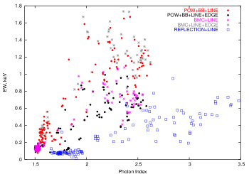
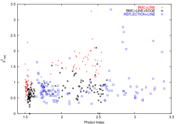
Figure 2: Performance of different XSPEC models in a subset of Cyg X-1 RXTE data. Left hand panel for EW vs photon index and right hand panel for $\chi^{2}$ vs photon index

An alternative mechanism for the line formation is proposed by Laming & Titarchuk (2004), LaT04 hereafter. In their scenario the iron line is formed in outflowing wind material. It is important to note that an absorption edge is physically required to compensate for absorption of photons above the K-threshold energy [see Kallman et al. (2004)] . Our results favor this model as it is consistent with equivalent width (EW) - spectral index correlations and is capable of accounting for high EW values. To illustrate our arguments and to investigate the mutual dependence of predicted spectral properties on the specific model we fit the subset of Cyg X-1 observations which includes low/hard, soft states and transitions between them. The models and the results of fits are presented on Figure 2. The power law plus blackbody empirical model and BMC model provide qualitatively similar results when the gaussian is used with the edge and without it. Considering the restricted RXTE energy resolution at low energies the exact values of gaussian EWs have to be handled with care. However, statistically the edge is highly significant. In Figure 3 we demonstrate the consistency of the our spectral model using a representative spectrum from Cyg X-1. For all fits we fix and relate the line energy at 6.4 keV to K threshold energy at 7.1 keV [see details of this relation in Kallman et al. (2004)]. To account for interstellar absorption we use a fixed hydrogen column of $N_{H}=0.5\times 10^{22}$ cm^-2.

Finally, according to the above arguments, the XSPEC model for the spectral fitting reads as WABS(GAUSSIAN+BMC)*EDGE. We use $\alpha$, the disk color temperatures, disk blackbody normalizations as free parameters of the spectral continuum model. The spectral fits was obtained using 3.5-30.0 keV energy range. We add 0.5% error to the data to account for systematic uncertainty in the PCA calibration. The typical quality of fit is good with $\chi^{2}_{red}$ in the range of 0.5-1.5.

3 Data Analysis Results and The Inferred Model Parameters

3.1 The evolution of the energy spectra in Cyg X-1

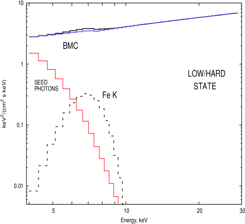
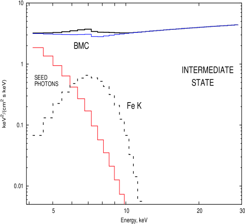
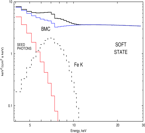
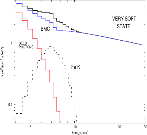
Figure 4: Spectral evolution of the source from low/hard state (panel a), through intermediate state (panel b) and soft state (panel c) to very soft state (panel d). Photon index of the upscattering Green function $\Gamma$ changes from 1.5 to 2.6 respectively.

The evolution of spectral properties of the source during the transition from the low/hard to the soft states is shown on Figure 4 and in Table 2. The temperature profile of the thermal (blackbody) component is plotted versus the index $\Gamma$ in Figure 5. This temperature is presumably related to the disk. It changes only slightly in the narrow range of 0.5 -0.6 keV and is nearly independent of the spectral state.

When the source is in the low/hard state the emerging radiation spectrum is presumably formed as a result of Comptonization of soft photons generated in the disk. We present a $\nu F_{\nu}$- diagram for the low/hard state in upper left hand panel of Figure 4 ($F_{\nu}$ is the energy flux). As a source progresses to higher luminosity states the spectrum becomes softer, the power-law part of the spectrum becomes steeper and the contribution of the blackbody (thermal) component increases. The strength of the iron line also increases (see the right upper panel in Figure 4). One can explain this evolution of the spectrum by an increasingly efficient deposition of the gravitational energy in the disk which becomes stronger towards the soft states (see e.g. Chakrabarti & Titarchuk, 1995; Esin et al., 1998).

The luminosity reaches the highest level in the soft state when the spectral index $\Gamma$ is about 2. The power-law plateau is clearly seen in $\nu F_{\nu}$- diagram presented in the lower left hand panel of Figure 4. Then, as the spectral index increases we observe a slight decrease in flux. We identify this phase as a very soft state (the so called “ thermal dominated state”), in addition to the canonical low/hard, intermediate and soft states. The energy spectrum is dominated by thermal component (more than 70% of total flux) and the maximum observed spectral index is $\sim 2.7$. It is important to emphasize that, typically, the high/soft state in the BH sources is observed when an extended power-law component has index $\Gamma\sim 2.7$ [see e.g. Grove et al. (1998), Borozdin et al. (1999), hereafter BRT99, TF04]. This relatively low index for Cyg X-1 soft state can be explained by a higher temperature of the converging flow than that for the high/soft state of other BH sources (see Laurent & Titarchuk, 2001, hereafter LT99, and also TF04). The main reason for this may be the fact that in the soft state of Cyg X-1, the energy release in the disk and in the Compton cloud are comparable while in the typical LMXB BH sources, like GRS 1915+105, XTE J1550-564, GRO 1655-40, in the high/soft state the energy release in the disk is much greater. When spectral index progresses to values higher than $\sim 2$ the luminosity decreases (see the lower right hand panel of Figure 4).

It is worth noting that we use a terminology for the spectral states in Cyg X-1 based on our physical scenario of the spectral evolution there (see more of the details in the discussion section). In our classification the difference between soft and very soft states corresponds to the difference in the spectral indices. In soft state when the saturation of the spectral index $\Gamma$ vs QPO frequency $\nu_{L}$ occurs, $\Gamma$ is about 2 (see §3.4). Whereas in the very soft state the spectra become softer and $\Gamma$ increases to the values of 2.7. No QPO frequencies are observed in this state.

In the scheme of McClintock and Remillard (2004) (and every other ”high” or ”very high state” BHC sources) this classification can look different. One should be careful in applying the definition of spectral states (particularly soft states) for some particular source.

3.2 The evolution of the power spectra in Cyg X-1

The next important question is how this spectral evolution is related to the timing characteristics of the source. In our study of the power density spectrum (PDS), we reveal that the PDS features, break frequency $\nu_{b}$, and Lorentzian low-frequency $\nu_{L}$ and Q-value of the QPO frequency evolve and increase while the source progresses toward the soft state. But the QPO frequencies are completely washed out in the very soft state. Titarchuk et al. (2002), hereafter TCW02, predicted that when the source is embedded in the optically thick medium the QPO features must be absent in the PDS of the source because of photon scattering.

When the radiation from the central source passes through the surrounding cloud of optical depth $\tau_{0}$ and of radius $R$ the direct (unscattered) and scatterred fractions of the radiation are $\exp(-\tau_{0})$ and [$1-\exp(-\tau_{0})$] respectively. Consequently the rms amplitude of the direct component decreases exponentially with $\tau_{0}$. TCW02 show that the rms amplitude of the scattered component $B(\omega)$ for a given rotational frequency $\omega=2\pi\nu$ decreases as

$$B(\omega)\propto\exp(-2\chi),$$ (1)

where $\chi(\omega,\tau_{0})=\{[\pi\tau_{0}/2(\tau_{0}+2/3)]^{4}+(3R\tau_{0}\omega/4c)^{2}\}^{1/2}$.

As seen from equation (1), the QPO amplitude of the radiation scatterred in the wind (cloud) decreases very rapidly with $\tau_{0}$ and with $\omega$ ($\nu$), namely

$$\chi\sim 4.7\left(\frac{\tau_{0}}{1}\right)\left(\frac{R}{10^{11}~{}{\rm cm}}\right)\left(\frac{\omega}{2\pi\times 0.3~{}{\rm Hz}}\right)\gg 1.$$ (2)

A radius R of $10^{11}$ cm was chosen as a typical radius of the wind inferred from the observations [Gies et al. (2003)] and theoretically inferred using luminosity and spectrum as observable characteristics of the source [Laming & Titarchuk (2004)].

Thus we can conclude that the variability of the scatterred part of radiation is completely washed out in the wind of radius of order $10^{11}$ cm even for $\tau_{0}{{}_{>}\atop{}^{\sim}}0.5$. The variability of the direct (unscattered) component is preserved but its rms amplitude decreases as $\exp(-\tau_{0})$ with $\tau_{0}$.

The power spectrum analysis of Cyg X-1 data confirms this expectation (see Pottschmidt et 2003; Axelsson, Borgonovo & Larsson 2005 and our results in this paper). The power spectrum in the very soft state is featureless (see Fig. 6). The emission of the central source is presumably obscured by the optically thick wind and consequently all photons emanating from the central source are scattered. The direct component of the central source radiation that carries information about the variability is suppressed by scattering. Gies et al. (2003) argue that there is a particular state of Cyg X-1 when the wind velocity is very low and thus one can expect high accumulation material in the wind and high optical depth of the wind. The wind downscattering of the photons emanating from the inner Compton cloud leads to the softening of spectrum (Titarchuk, & Shrader, 2005) and consequently to a decrease in X-ray luminosity of the source. The softening of the spectrum can also be a result of effective cooling the Compton cloud by the disk soft photons. If the power law component of the soft state is formed in the converging flow, then the high indices are a result of the low flow temperature (LT99). The index increases and saturates to the critical value about 2.8 with the mass accretion rate for the low temperatures of the flow (see LT99 and Titarchuk & Zannias 1998, hereafter TZ98).

To calculate the power spectrum of the central source emission affected by scattering one should present the quantitative model of the resulting pulse affected by scattering $z(t)$ which can be written as follows:

$$z(t)=\int_{0}^{t}x(t^{\prime})g(t-t^{\prime})dt^{\prime},$$ (3)

where $x(t)$ is the input pulse of the central source oscillations and $g(t)$ is the response pulse of the scattering medium. The power spectrum of $z(t)$ is a product of the power spectrum of $x(t)$ and $g(t)$, i.e.

$$||F(\omega)||^{2}=||F_{cs}(\omega)||^{2}||F_{scat}(\omega)||^{2},$$ (4)

where

$$F(\omega)=\int_{0}^{\infty}e^{-i\omega t}z(t)dt,$$ (5)

$$F_{cs}(\omega)=\int_{0}^{\infty}e^{-i\omega t}x(t)dt,$$ (6)

$$F_{scat}(\omega)=\int_{0}^{\infty}e^{-i\omega t}g(t)dt$$ (7)

are Fourier transforms of $z(t),~{}x(t),~{}G(t)$ respectively. The time response of the innermost part of the source $x(t)$ can be considered in terms of diffusion propagation of perturbation in the disk transition layer (TL). Any local perturbation in TL (bounded medium) would propagate diffusively outward over time scale (see TL99)

$$t_{dif}\sim\frac{l_{fp}}{v}\left(\frac{L}{l_{fp}}\right)^{2}=\tau_{pert}\frac{L}{v},$$ (8)

where $L=R_{out}-R_{in}$ is the characteristic thickness of the TL, $l_{fp}\sim\eta/(\rho v)=(\sigma_{pert}n)^{-1}$ is the mean free perturbation path related to the turbulent MHD viscosity $\eta$, the matter density $\rho$, the number density $n$ and the perturbation interaction cross-section $\sigma_{pert}$ in the TL and $\tau_{pert}=L/l_{fp}=\sigma_{pert}nL$. Even though the specific mechanism providing this viscosity needs to be understood, this time scale $t_{dif}$ apparently “controls” the diffusion supply of the matter into the innermost region of the accretion disk (TL).

The response function $x(t)$ is a solution the time-dependent problem for perturbation diffusion that mathematically is formulated as an initial value problem for the diffusion equation in the bounded medium (see more details of the diffusion theory in ST80, ST85, T94). This solution is a linear combination

$$x(t)=\sum_{k=1}^{\infty}A_{k}e^{-\lambda_{k}^{2}t/3t_{fp}},$$ (9)

where $t_{fp}=l_{fp}/v$ is a free path crossing time, $t_{k,diff}=(\lambda_{k}^{2}/3t_{fp})^{-1}$ is kth eigen diffusion time, $A_{k}=c_{k}X_{k}(R_{out})$, $c_{k}$ is expansion coefficient of the source perturbation function $f(r)$

$$c_{k}=\frac{\int_{R_{in}}^{R_{out}}\varphi(r)X_{k}(r)f(r)dr}{{\int_{R_{in}}^{R_{out}}\varphi(r)X_{k}^{2}(r)dr}}$$ (10)

that is related to eigenvalues $\lambda_{k}$ and eigen functions $X_{k}(r)$ of the appropriate space diffusion operator and $\varphi(r)$ is the operator weight function.

If $\tau_{pert}{{}_{<}\atop{}^{\sim}}1$ then the response function as a solution of the diffusion problem can be presented by a single exponent, namely

$$x(t)\approx A_{1}e^{-\lambda_{1}^{2}t/3t_{fp}}=A_{1}e^{-t/t_{cs}},$$ (11)

because in this case $\lambda_{1}^{2}/3\sim 1/\tau_{pert}^{2}{{}_{<}\atop{}^{\sim}}1$ and $\lambda_{1}^{2}/3\ll\lambda_{k}^{2}/3$, for $k=2,3,...$, where $t_{cs}=t_{1,diff}=(\lambda_{1}^{2}/3t_{fp})^{-1}$ (ST80, ST85, T94).

The scattering response function $g(t)$ is a solution of the diffusion problem for the photon scattering in the extended envelope (wind) that surrounds the central source. The formula for the photon diffusion time $t_{scat}$ is very similar to formula (8), i.e.

$$t_{scat}\sim\tau_{0}\frac{L_{w}}{c},$$ (12)

where $L_{w}=R_{w,out}-R_{w,in}$ is the envelope thickness and the Thomson optical depth of the envelope $\tau_{0}=\sigma_{\rm T}n_{e}L$. When $\tau_{0}{{}_{<}\atop{}^{\sim}}1$ (similarly that for the perturbation diffusion) the scattering diffusion function $g(t)$ can be presented by the exponent

$$g(t)\approx A_{1,w}e^{-t/t_{scat}}.$$ (13)

It is worth noting that $t_{scat}\gg t_{cs}$, because $L_{w}\gg L$ by definition of $L_{w}$ and $L$.

For these particular response functions (see Eqs. 9, 13) the power spectra are

$$||F_{cs}||^{2}\propto(\omega^{2}+t_{cs}^{-2})^{-1},$$ (14)

$$||F_{scat}||^{2}\propto(\omega^{2}+t_{scat}^{-2})^{-1},$$ (15)

and

$$||F||^{2}=||F_{cs}||^{2}||F_{scat}||^{2}\propto(\omega^{2}+t_{cs}^{-2})^{-1}(\omega^{2}+t_{scat}^{-2})^{-1}.$$ (16)

Because $t_{scat}\gg t_{cs}$ we have the following asymptotics for the power spectrum $||F||^{2}(\nu)$ as a function of $\nu~{}(=\omega/2\pi$)

$$||F||^{2}(\nu)\propto(t_{cs}t_{scat})^{2}\nu^{0}~{}~{}~{}~{}~{}~{}~{}~{}~{}~{}~{}~{}~{}~{}~{}~{}~{}~{}~{}~{}~{}~{}{\rm for}~{}~{}\nu\ll 1/(2\pi t_{scat})$$ (17)

$$||F||^{2}(\nu)\propto(t_{scat}/2\pi)^{2}\nu^{-2}~{}~{}~{}~{}~{}~{}{\rm for}~{}~{}1/(2\pi t_{scat})\ll\nu\ll 1/(2\pi t_{cs})$$ (18)

$$||F||^{2}(\nu)\propto(2\pi)^{-4}\nu^{-4}~{}~{}~{}~{}~{}~{}~{}~{}~{}~{}~{}~{}~{}~{}~{}~{}~{}~{}~{}~{}~{}{\rm for}~{}~{}\nu\gg 1/(2\pi t_{cs}).$$ (19)

In Figure 6 one can clear see the change of the power-law index of the $\nu\times$power diagram from $(0)$ to $(-2)$ about 0.08, 0.5, 3 Hz in the low/hard, intermediate and the soft states respectively. Thus one conclude that the perturbation diffusion times in the TL (Compton cloud) $t_{dif}\sim 1/(2\pi\nu_{b}$ Hz) are about $2,~{}0.3,~{}0.05$ s in these states.

The change of the power-law index of the diagram from (1) to (-1) [that corresponds to 0 -(-2) changes of that in the power spectrum (Eqs. 17, 18)] takes place in the low-frequency parts of the diagrams for the low/hard, intermediate and soft states (black, blue, red respectively). The power at high frequencies decays very fast and the corresponding power-law index of PDS is about 4 (see Eq. 19).

However in the $\nu\times$power diagram for the very soft state the index changes from 0 to (-1) at low-frequency (about 0.2 Hz) but this change is not described by aforementioned formulas (16, see also 17, 18). We argue this particular power-law index transition occurs in the source when the optical depth of the wind $\tau_{0}\gg 1$.

In order to demonstrate this effect one must calculate the power spectrum of the scattering response function $g(t)$ for $\tau_{0}\gg 1$. The derivation of these formulas are out of scope of the paper and we shall present these results elsewhere.

It is worth commenting that we have already shown here, the resulting power spectrum is a product of two power spectra related to the disk PDS and another one to Compton cloud (scattering) PDS (see Eq. 4). In the general case, each of these spectra is a power spectrum of the series of eigen exponential shots [see for example, formula 9 for $x(t)$]. For frequencies much less than the characteristic scattering frequency, $\nu\ll\nu_{scat}=1/(2\pi t_{scatt})$ the resulting spectrum is represented by a power-law red noise component. In our simple treatment of this problem considered here and applicable to the hard and intermediate states only (see Eq. 16) the low-frequency power-law index of PDS is zero. In fact, the index and power-law cuttoff frequency increases with mass accretion rate when the source undergoes transition to a soft state. We shall provide all details of this correlation in a future publication.

3.3 Correlation of K_α line strength with the photon index

Another observational appearance of the wind is the strong broad feature of K_α line in the spectrum that is present in all spectral states of Cyg X-1 (see Fig. 4). In Figure 7 (upper panel) we demonstrate how equivalent width EW of the K_α line increases with the photon index $\Gamma$ from about 150 eV in the low/hard state to about 1.3 keV in the high/soft and very soft states. One can see signs of saturation of the EW at about 1.3 keV for indices above 2.1 when no QPO is present in the power spectrum. Wilms et al. (2005) have also found that one needs a strong K_α line for fitting data with a Comptonization model (CompTT). The strength of the line increases almost linearly with a accretion disk flux until it satures at the values of $\sim 1$ keV.

The X-ray photons presumably originated in the innermost part of source, in an area less than 40 Schwarzschild radii, illuminate the wind. In this case the wind gas is heated by Compton scattering and photoionizations from the central object. It is cooled by radiation, ionization, and adiabatic expansion losses (LaT04). The photons above the K-edge energy are absorbed and ionize iron atoms that leads to the formation of the strong K_α line. LaT04 calculated ionization, temperature structure and the equivalent widths of Fe K_α line formed in the wind. For the wide set of parameters of the wind (velocity, the Thomson optical depth $\tau_{\rm T}$) and the incident Comptonization spectrum (the index and the Compton cloud electron temperature) they established that EW of the line should be about 1 keV and less for the line to be observed. LaT04 also predicted that for this case the inner radius of the wind should be situated at $(10^{3}-10^{4})/\tau_{0}$ Schwarzschild radii away from the central object.

In the framework of the wind model we can inferred the optical depth of the outer shield (wind) as a function of the index using the EW of K_α line [see Basko (1978), CT95]:

$$EW=\omega_{K}\int_{E_{th}}^{\infty}(E/E_{th})^{-\alpha}\{1-\exp[-(Y+Y_{0})\tau_{0}(7.8~{}{\rm keV}/E)^{3}]\}dE.$$ (20)

where $\omega_{K}$ is the fluorescence yield, $E_{th}$ is the K shell ionization threshold energy, $Y$ and $Y_{0}$ are the abundances of elements (in units of the cosmic abundances) with a charge $Z<26$ and the iron abundance, respectively. This integral can easy be calculated using the following formula

$$EW=7.8~{}{\rm keV}\times\omega_{K}\sum_{m=1}^{\infty}(-1)^{m-1}\frac{[(Y+Y_{0})\tau_{0}]^{m}}{(3m+\alpha-1)m!}\left(\frac{7.8~{}{\rm keV}}{E_{th}}\right)^{3m-1}.$$ (21)

We apply the value of $E_{th}\sim 7.1$ keV [see Kallman et al. (2004)], and $\omega_{K}=0.34$ [see Bambynek et al. (1972)]. In Figure 7 (lower panel) we present the inferred dependence of $\tau_{0}(Y+Y_{0})$ on the photon index.

To obtain a description of the X-ray photon spectrum of Cyg X-1 many authors (see e.g. Gilfanov, Churazov & Revnivtsev 1999, hereafter GCR99; P03) used an empirical model in which each source spectrum is a sum of power law spectrum with photon index $\Gamma$ and a multi-temperature disk blackbody (Makishima et al. 1986). To this continuum, a reflection spectrum after MZ95 was added. GCR99 emphasized that this empirical model is obviously oversimplified and therefore the best-fit parameter values do not necessarily represent physically meaningful quantities. Particular problems arise with the values of the reflection factor $R=\Omega/2\pi$ and the equivalent width of the iron line. The best-fit values of $R=\Omega/2\pi$ for the soft state exceed the unity considerably $(R=1-5)$, which is physically meaningless in the geometry of the reflection. In fact, Lapidus, Sunyaev & Titarchuk (1985), showed that the maximum reflection factor for geometrically thin infinite disk illuminated by isotropic radiation from the central object is 0.25.

The values of the EW of K_α inferred by GCR99 vary from 80 to 300 eV. These EWs are related to the line component included in the spectrum in addition to the refelection component. Because the reflection model includes its own iron line component (MZ95) thus the actual strength of the line is much higher in Cyg X-1 than that presented in GCR99. One can determine that the total iron line strength strongly increases with photon index because of the power of the so called “reflection component” R, which also strongly increases with the index (see Figs 5, 8 in CGR99). In this sense our inferred strong lines in the soft states of Cyg X-1 agree with those in GCR99.

3.4 The index-QPO correlation

In Figure 8 we present the correlation of photon index $\Gamma$ versus low QPO frequency $\nu_{L}$ (orange points in the upper panel) and the correlation of $\Gamma$ versus break frequency $\nu_{b}$ (the lower panel) observed in Cyg X-1.

We compare the index-QPO correlation with those observed in GRS 1915+105, XTE J1550-564. One notices similar properties for all of these sources: i. when QPO is detected the photon index does not go above 3, ii. the index saturates. at low and high values of the QPO frequencies. In Cyg X-1 the saturation level of the index for high values of low QPO frequency is remarkably lower than for the other two sources.

TF04 argues that the index saturation level is determined by the temperature of the converging flow where the soft (disk) photons are upscattered by electrons to the energy of falling electrons (LT99). In principle, one can evaluate the mass of the central BH using the index-QPO relation because QPO frequencies are inversely proportional mass (TF04). The simple slide of the index-QPO correlation for XTE J1550-564 (pink line) over the frequency axis gives us the index-QPO correlation for GRS 1915+105 (blue line). The shifting factor is 10/12 which gives the relative BH mass in XTE J1550-564 with respect to that in GRS 1915+105. But one caveat should be taken into account: this sliding method works if the index-QPO relations are self-similar with respect to each other as occurs for GRS 1915+105 and XTE J1550-564.

3.5 Flux-index and Comptonization fraction-index relation

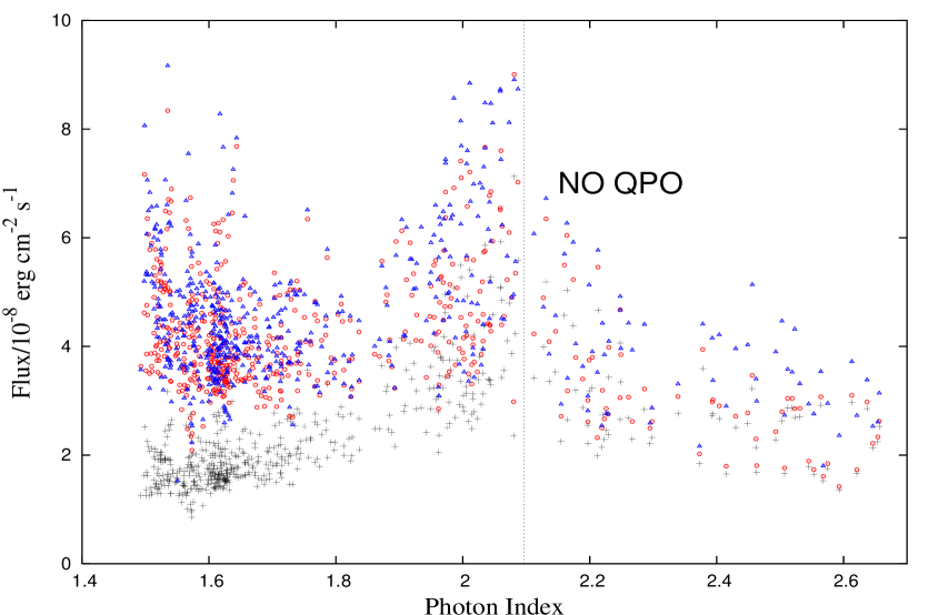
Figure 9: Flux in the energy band from 1 keV to 30 keV (black crosses) as a function of the index $\Gamma$. Bolometric corrected flux (1-300 keV) is shown in red circles. Blue triangles is a total flux inferred from the Comptonization enhancement factor ${\cal E}_{\rm Comp}$. The total fluxes given by bolometric correction and Comptonization model show excellent consistency. The 1-30 keV flux gradually increases toward the soft state with ($\Gamma\sim 2.1$), while the total flux stay almost constant, only slightly increasing during this soft state. In the very soft state ($\Gamma>2.1$, no QPO detected) the flux sharply drops with the index presumably due to downscattering of X-ray emission of the central source in the strong wind.

In Figure 9 we show how the 1-30 keV flux (black crosses) varies during the spectral transition from the low/hard state (L/H) to very soft (VS) state. We use joint PCA/HEXTE spectral fits for bolometric corrections for high energies. We extracted HEXTE spectra from Cluster A and Cluster B using the same screening criteria that we obtained for PCA spectra. To fit PCA/HEXTE data we apply the model obtained for PCA multiplied by high energy cutoff (HIGHECUT) component to account for high energy turnover in the hard tail of the X-ray spectrum. The flux is then calculated by integrating the best-fit model spectrum over the energy interval from 1 keV to 300 keV. Absolute normalization of HEXTE data for both clusters were allowed to change free with respect to PCA normalization. The resulting fits show the HEXTE normalization consistently less than the normalization for PCA by 15-20% as expected. Resulting values of bolometric flux are shown on Figure 9 (red circles).

We confirmed Zhang’s et al. (1997) claims that the bolometric flux remains almost unchanged (within 50%, almost) during L/H to VS transition. This phenomenon can be explained as a combined effect of the mass accretion rate increase and the Comptonization enhancement decrease when the system undergoes the spectral transition. In the low/hard state the relative small energy release (low mass accretion rate) in the disk is compensated by high Comptonization efficiency in the corona while in the very soft (thermal dominated) state the situation is opposite. Sunyaev & Titarchuk (1980), hereafter ST80, and Sunyaev & Titarchuk (1985), hereafter ST85, derive the asymptotic form of the Comptonization enhancement factor ${\cal E}_{\rm Comp}$ for both regimes of the energy spectral index ($\alpha<1$ and $\alpha\geq 1$). Chakrabarti & Titarchuk (1995), hereafter CT95, provides the general formula for ${\cal E}_{\rm Comp}$ (CT95, formula 14) which combines these two asymptotic. In order to infer the bolometric flux dependence $F_{bol}$ on the photon index using the observable thermal (disk) flux $F_{th}$ one should multiply $F_{th}$ by $[1+(A/(A+1)){\cal E}_{\rm Comp}]$ and apply formula (14) in CT95 for ${\cal E}_{\rm Comp}$, namely

$$F_{bol}=F_{th}\left[1+\frac{A}{1+A}{\cal E}_{\rm Comp}(\alpha,x_{0})\right],$$ (22)

where $x_{0}=2.7kT_{col}/kT_{e}$, $kT$ is a color temperature of disk radiation (see Fig 5) and $kT_{e}$ is electron temperature of Compton cloud. The enhancement factor ${\cal E}_{\rm Comp}$ depends on $kT_{e}$ only for $\alpha<1$ ($\Gamma<2$) (see formula 14 in CT95).

In order to infer $kT_{e}$ we apply use the same PCA/HEXTE data. To calculate the electron temperature $kT_{e}$ we use the HIGHECUT parameter, $E_{fold}$ and well-known relation between the electron temperature and the high energy cutoff of the Comptonization spectrum, namely $kT_{e}\approx E_{fold}/2$ (see e.g. ST80 and T94). We present the results of calulations of ${\cal E}_{\rm Comp}(\alpha,x_{0})$ as a function of $\Gamma(=\alpha+1)$ for different values of $kT_{col}$ (see Fig. 10).

In Figure 9 we demonstrate a dependence of $F_{bol}$ on the photon index $\Gamma(=\alpha+1)$ (blue triangles). The theoretically predicted and observed flux values are in good agreement along. Thus the inferred luminosty-index relation supports the idea that the variation of luminosity with index is due to the combined effect of the disk mass accretion rate and Comptonization of the disk photons in the corona.

The soft photon radiation is completely Comptonized in the low/hard state while the relative contribution of the Comptonized radiation decreases toward the very soft (thermal dominated) state. In Figure 11 we present the observed correlation between the ratio of the Comptonized flux to the bolometric flux and the index. The Comptonized spectrum is a convolution of the soft photon spectrum with the upscattering Comptonization Green’s function. This component of the observable spectrum and consequently the related flux can be obtained using the BMC model. The inferred Comptonized fraction of the spectrum helps us to reveal the relative size of the corona (Compton cloud) with respect to the disk emission region. One can see that in the soft states the coronal region becomes more compact. This effect is also confirmed by the observed index-QPO correlations (see Fig. 8). The QPO frequencies increases with the index as a result of the mass accretion rate increase. In fact, the coronal region is pushed close to BH when mass accretion rate goes up (see TLM98 and TF04). In the soft states (when the Compton cloud is relatively cold) the converging flow site (${{}_{<}\atop{}^{\sim}}3-4R_{\rm S}$) is only the place where the soft (disk) photons get scattered due to the dynamical Comptonization.

3.6 Break frequency- QPO low frequency relation and BH mass determination

In Figure 12 we present the observed correlation between the break frequency $\nu_{b}$ and the low frequency $\nu_{L}$. We fit this correlation by the broken power law of the form

$$\nu_{b}=a(\nu_{L}/\nu_{\ast})^{\beta_{1}}~{}~{}~{}~{}{\rm for}~{}~{}~{}~{}\nu_{L}<\nu_{\ast}~{}~{}~{}{\rm and}~{}~{}~{}~{}\nu_{b}=a(\nu_{L}/\nu_{\ast})^{\beta_{2}}~{}~{}~{}~{}{\rm for}~{}~{}~{}~{}\nu_{L}\geq\nu_{\ast}.$$ (23)

The best-fit parameters: the normalization $a\sim 0.32$, the “low”-frequency index $\beta_{1}\sim 1$ and the “high” frequency index $\beta_{2}\sim 1.65$ and the “boundary” index $\nu_{\ast}=2.2$ Hz. Titarchuk, Osherovich & Kuznetsov (1999) found that the “high” frequency index $\beta_{2}\sim 1.6$ is a canonical index of break-low frequency correlation for a quite a few BH and NS sources. In fact, Titarchuk & Osherovich (1999) identified using dimensional analysis the corresponding radial oscillation and diffusion frequencies in the transition layer (TL) with the low-Lorentzian $\nu_{L}$ and break frequencies $\nu_{b}$ for 4U 1728-34. They predicted values for $\nu_{b}$ related to the diffusion in the transition layer, that are consistent with the observed $\nu_{b}$. TO99 argue that $\nu_{L}$ is the inverse of the oscillation time of the TL radial mode,

$$\nu_{L}=C_{bd}\frac{v}{L}\sim t_{QPO}^{-1}$$ (24)

and $\nu_{b}$ is the inverse of the diffusion time of the perturbation propagation in the TL

$$\nu_{b}=\frac{v}{f\tau_{pert}L}\sim t_{dif}^{-1},$$ (25)

where $L$ is the TL radial size (see definition of $\tau_{pert}$ in the text after Eq. 8). $C_{bd}$ is the coefficient which depends on the specific outer and inner boundary conditions imposed in the TL (see, Titarchuk, Bradshaw & Wood 2001, for details of the boundary problem of the diffusion and oscillations in TL). Diffusion time $t_{dif}$ is related to the diffusion length $L_{dif}=l_{fp}N_{int}$ where $l_{fp}$ is a free propagation path of the perturbation in the TL, $N_{int}=f(L/l_{fp})^{2}=f\tau_{pert}^{2}$ is a number of matter interactions, related to the effective viscosity in the TL. Factor $f$ is related to the source distribution of the perturbation in the TL (see Sunyaev & Titarchuk 1985 for details). Thus the relation between $\nu_{b}$ and $\nu_{L}$ reads as follows

$$\nu_{b}=\frac{1}{f\tau_{pert}}\nu_{L}.$$ (26)

Because the perturbation dimensionless depth $\tau=L/l_{fp}$ is related to $L$ then

$$\nu_{b}=\frac{1}{f\tau_{pert}}\nu_{L}=\frac{C_{bd}l_{fp}v}{fL^{2}}.$$ (27)

Thus one can find taking into account Eqs.(24, 27) that $\nu_{b}$ should not be a linear function of $\nu_{L}$ if $f\tau_{pert}\gg 1$. TO99 found that $\nu_{b}\propto\nu_{L}^{1.6}$ when $\tau_{pert}\gg 1$. The number of interactions in the TL hydrodynamical flow $N_{int}$ and the perturbation depth $\tau_{pert}=L/l_{fp}$ depends strongly on the mass accretion rate. For relatively high rates one should expect that $N_{int}\gg 1$ and $f\tau\gg 1$ while these values are about one for relatively small mass accretion rates that occur in the low/hard state. In the latter case the dependence of $\nu_{b}$ on $\nu_{L}$ is almost linear.

This diffusion effect is confirmed by the correlation of $\nu_{b}$ and $\nu_{L}$ observed in Cyg X-1 (see Fig 12). For higher values of frequencies $\nu_{b}$ ans $\nu_{L}$ (which correspond to higher values of mass accretion rate) $\nu_{b}\propto\nu_{L}^{1.6}$ while for lower values $\nu_{b}\propto\nu_{L}$.

The low frequency $\nu_{L}$ is inversely proportional to the TL size which its turn is proportional to the mass of the central object $m=M/M_{\odot}$ (BH or NS). Thus one can conclude that $\nu_{L}$ and $\nu_{b}$ are inversely proportional to m when mass accretion rate in a source is relatively small. This inverse proportionality of $\nu_{b}$ vs $m$ can be used for the mass determination of the objects that mass differs by order of magnitude from Galactic BHs for example, of the supermassive or intermediate BHs provided the break frequency is detected there. Recently, Fiorito & Titarchuk (2004) applied rescaling of QPO frequency $\nu_{L}$ to evaluate a BH central mass in ultraluminous source M82 X-1 while McHardy et al. (2005) and Dewangan, Titarchuk & Griffiths (2006) applied rescaling of $\nu_{b}$ for the BH mass determination in AGN and ULX respectively.

4 Conclusions and Discussion

We have presented a detailed spectral and timing analysis of X-ray data for Cyg X-1 collected with the RXTE. We find observational evidence for the correlation of spectral index with low-frequency features: $\nu_{b}$ and $\nu_{L}$. The photon index $\Gamma$ steadily increases from 1.5 in the low/hard state to values exceeding 2.1 in the soft state. The low frequency $\nu_{L}$ is detected throughout the low/hard and intermediate states, while it disappears when the source undergoes transition to the very soft (thermal dominated) state. Like in other BH sources, there is an indication of saturation of the index in the soft state for Cyg X-1 (see Fig.8). This saturation effect, which is presumably due to photon trapping in the converging flow, can be considered to be a BH signature. We want to stress that this saturation is a model independent phenomenon found in the present analysis of X-ray RXTE data. On the other hand, the saturation of the index with mass accretion rate increase (which is strongly related to the QPO frequency increase) has to apply to any BH, because the photons are unavoidably trapped in the central accretion flow. It is a necessary condition of BH presense in the accreting systems.

Thus the index saturation with QPO frequency seen in the source (rather than the presense of the tail in the soft state) is a signature of the horizon. In fact, one can see high energy tails with indices at about the BH saturation value 2.8 in the high/soft state observations of weakly magnetized accreting NS binaries, for example GX 17+2 (Farinelli et al. 2005) and 4U 1728+34 (TSh05). Farinelli et al. (2005) presented two spectra of GX 17+2 observed in 1997 by BeppoSAX. Using these spectra alone one cannot establish the evolution of the indices with the mass accretion rate. TSh05 analyzing $\sim 1.5$ Ms of RXTE archival data for 4U 1728-34 reveal the spectral evolution of the Comptonized blackbody spectra and QPO frequencies when the source transitions between hard to soft states. Contrary to the BH sources, the indices of 4U 1728-34 spectra do not saturate as QPO frequency increases. They increase from $\sim 2$ (in the hard state) to $\sim 6$ (in the soft state) with no signature of saturation versus QPO frequency (or mass accretion rate). The NS soft state spectrum consists of two blackbody components that are only slightly Comptonized (inferred photon indices of the Comptonization Green’s function are $\Gamma{{}_{>}\atop{}^{\sim}}6$). Thus one can claim (as expected from theory) that in NS sources thermal equilibrium is established for high mass accretion rate (soft) state. In BHs the equilibrium is never established because of the presence of the event horizon. The emergent BH spectrum, even in the soft state, has a power-law component which index saturates with mass accretion rate. It is worth noting that there is a particular state in BH source when it can show signs of the thermal equilibrium: the emergent spectrum consists of one or two thermal components. But no QPO is observed then. In this (very soft, thermal dominated) state the source is presumably covered by a powerful wind that thermalizes the radiation of the central source and prevents to see any QPO generated in the source (see Fig. 6).

One can argue that the bulk motion Comptonization (BMC) is ruled out as a main radiative process in the soft spectral states of black-hole binaries because of the inefficiency of producing photons with energies ${{}_{>}\atop{}^{\sim}}100$ keV and the lower relative normalization of the BMC component (see a recent paper by Niedzwiecki & Zdziarski 2005 on Monte Carlo simulation of the bulk motion Comptonization, hereafter NZ05). The production of high energy photons in Monte Carlo simulation with steep power-laws ($\Gamma>2$) is a technically difficult problem because of poor statistics. It requires a long simulations and special methods for the treatment of the poor statistics at high energies. LT99 implemented this technique and found in their simulations that the spectra extend up to 200-300 keV. In fact, NZ05 do not show histograms of their simulated spectra but rather show the best-fit curves describing results of their simulations. It is impossible to quantify uncertainties and the quality of counting statistics as a function of energy in the NZ05 simulations.

The absolute normalization of the Comptonized component is always determined by the seed photon normalization (illumination pattern). LT99 and then Turolla, Zane & Titarchuk (2001) and NZ05 confirm that the illumination pattern does not affect the shape of the BMC spectrum. Thus, the relative normalization of the Comptonized (BMC) with respect to that of blackbody is a model dependent parameter. LT99 show that the BMC normalization can be very high and comparable with the disk BB component when the innermost part the accretion flow (BMC area of 1-3 $R_{\rm S}$) is illuminated by the soft photons coming from the geometrical thick disk situated very close. The normalization is quite low when the seed photons illuminated the converging flow region come from the geometrically thin disk (see NZ05).

In contrast to the claim by NZ05, which is based on their spectral modeling, we find that Cyg X-1 observations show a very strong Bulk Motion Comptonization signature in the soft state as a photon index saturation with QPO frequency (mass accretion rate). This is a well-known signature of the photon trapping in the converging flow discovered by TZ98 and then confirmed in Monte Carlo simulations by LT99.

We also demonstrate that the Fe K_α line equivalent width correlates with spectral index and correspondingly with QPO frequencies when they are present in the data (see Figs. 7, 8). This leads us to conclude that the compactness of the X-ray emission area (taking the QPO frequency value as a compactness indicator) is higher for softer spectra (related to higher mass accretion rate). On the other hand the Fe K_α emission-line strength (EW) is about one keV when the power spectrum is featureless. It happens in the very soft (thermal dominated) state. Thus the observations may be suggesting that the photospheric radius of the Fe K_α emission is orders of magnitude larger than that for the X-ray continuum. We propose that Fe K_α line emission originates in the wind where the photons emanated from the central part of the source are downscattered by electrons and absorbed by partly ionized iron atoms.

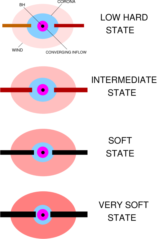
Figure 13: The inferred scenario of the spectral transition in Cyg X-1. Strength of disk and outflow (wind) increase towards the soft states.

In Figure 13 we present a scenario that is infered using our spectral and timing data analysis of Cyg X-1 spectral state transitions. In the low/hard state X-ray radiation comes from a relatively extended area. A Compton cloud covers the large portion of the accretion disk that generates soft photons. Most of these photons are upscattered in the hot Compton cloud. On its way to the observer some fraction of the Comptonized radiation is reprocessed in the relatively transparent cloud. Here Fe K_α line is formed because the photons of energy close to K shell ionization edge and higher are effectively absorbed and then remitted (with a certain probability) as K_α-photons. QPO features are not washed out by photon scattering in the wind shell in this state because the optical depth of the wind is less then 0.5 (see Fig. 7, lower panel). The wind becomes thicker in the intermediate and soft states and it is optically thick in the very soft (thermal dominated) state. This picture is supported by the fact that the oscillation amplitude and the QPO strength steadily decreases when the source proceeds to soft state and the QPO features are completely washed out in the very soft state (see Fig. 6). Also the strength of K_α (that is presumably generated in the wind) increases with the index (see Fig. 7, upper panel). On the other hand, the Compton cloud becomes very compact and cooler in softer states with respect to that in the low/hard state. The Compton cloud size approaches that of the converging inflow which is a few Schwarzschild radii. Also, in perfect agreement with our scenario, the inferred fraction of the Comptonized component in the emergent spectrum (see Fig. 11) decreases with the index (i.e. with mass accretion rate).

There several other studies of the X-ray spectral and timing properties of Cyg X-1 and other BHs which directly relate to the results of our paper. Particularly, Pottschmidt et al. (2003, P03) also found correlations between the photon index and QPO frequencies with a clear sign of the index saturation at high values of the (low frequency) QPO(see Fig. 7, panel b in P03). We found that our QPO frequencies $\nu_{L}$ and QPO frequencies $\nu_{3}$ in P03 are almost identical and they show the similar correlations with the photon index $\Gamma$. P03’s frequencies $\nu_{2}$ are presumably very close to our break frequency $\nu_{b}$.

To obtain a description of the X-ray photon spectrum, P03 like many other authors (see e.g. GCR99) used an empirical model in which each source spectrum is a sum of power law spectrum with photon index $\Gamma$ and a multi-temperature disk blackbody. To this continuum, a reflection spectrum after MZ95 was added. GCR99 emphasized that this empirical model is an oversimplification and therefore the best-fit parameter values do not necessarily represent the physically meaningful quantities.

GCR99 also showed that the reflection model can properly mimic the reprocessed component of the spectrum. Particularly for intermediate and soft states (when $R>1$ in the reflection modeling) one can clearly see the high strength in the fluorescent K_α iron line at 6-7 keV and the deep broad smeared iron K-edge at $\sim 7-10$ keV (see Figs. 6-7 in GCR99). We confirm GCR99’s conclusions that these line and K-edge edge features are more pronounced towards soft states. However, we argue that these spectral features are results of reprocessing of the central source hard radiation in the outflow warm absorber (wind) that surrounds the central BH. This our claim is supported by observed QPO power decay towards the softer states that is presumably a result of reprocessing of time signal in the extended relatively warm wind (see Fig 6).

Recently Proga (2005) and Proga & Kallman (2004) demonstrated using the results of hydro simulations, that the disk illumination by the radiation of the central source or just local disk luminosity can launch a wind off the disk photosphere. They argue that radiation pressure due to UV (line resonances) couples the X-ray and UV radiation processes by driving the disk material above the disk where the most part of the X-ray emission of the central source propagates. A strong disk wind develops when the local disk flux $L_{D}$ is more than 0.3 $L_{\rm Edd}$. For a less luminous disk the line force can still force material off the disk but it fails to accelerate the flow to escape velocity.

One should stress that the timing and spectral data do reveal signatures of reprocessed component of the hard radiation in terms of high iron line equivalent width (about one keV in the soft states) and broad iron K-edge features. The strengths of these features seen in the observations strongly exclude their formation by disk reflection. The highest value of EW due to reflection must be less than 100 eV (see Basko 1978 and George & Fabian 1991). In fact, the best-fit values of the reflection scaling factor $R=1-5$ inferred from the Cyg X-1 observations contradict to the basic assumption of the reflection model for which $R$ cannot be more than 0.25. As a result of our data analysis we have also found using the reflection model by MZ95 that $R$ correlates with spectral index and values of $R$ are as high as $6$ at $\Gamma\sim 3.4$ (see Fig 14).

In principle, the reflection effect from outer relatively cold parts of the disk would be detected in the low state of the source when the spectrum is relatively hard (photon index $\Gamma\sim 1.5$). In this case one can see a reflection hump in the spectrum around 10-15 keV (ST80). The main problem with the detection of this feature along with low EW of the line is that the fraction of reflected emission $f$ in the resulting spectrum is about 8% and less, i.e. $f=R\cdot A{{}_{<}\atop{}^{\sim}}0.25\cdot 0.3=0.075$ where $A{{}_{<}\atop{}^{\sim}}0.3$ is albedo of the cold material (Basko, Sunyaev & Titarchuk 1974, Titarchuk 1987). Such tiny reflection features will be readily washed out by intervening wind clouds (see above). The disk reflection effects become much weaker for softer spectra (states), for which photon index more than 2. Thus the strong iron and K-edge features detected in the soft state are likely not due to reflection from the disk at all. Rather they should be formed in the extended wind clouds surrounding the central black hole. The relative large time lag observed in the soft state (see GCR99) really corroborate this scenario of reprocessing of the spectrum of the central object in the very extended environment (wind) of the source.

McConnell et al. (2002) using GRO/COMPTEL observations of Cyg X-1 claim that the high energy tail in the soft state shows no cutoff up to at least 0.5 MeV and 10 MeV respectively. They demonstrate that their analysis from BATSE, OSSE and COMPTEL show that the combined spectrum can be described by a single power law with a best-fit photon index of $\Gamma=2.58\pm 0.03$. For these particular states for which $\Gamma>2.1$ RXTE power spectra are featureless (see Fig. 6), no QPOs are seen in these states. In fact, Grove (2005, private communications) confirms that OSSE power spectra of Cyg X-1 also do not show any signatures of QPO but only red noise. It means that in these observations the central BH is not seen directly but through a very extended cloud that ultimately washes out the timing and spectral information of the central object. It is also worth pointing out that the COMPTEL exposure time is about $6\times 10^{6}$ s that is much longer than the spectral formation time near the central black hole(which is of order of crossing time of the innermost part of BH, a few times of $10^{7}{\rm cm}/c\sim 10^{-3}$ s). The hydrodynamical time scale can be longer by two orders of magnitude than the spectral formation time but it is still 7 orders of magnitude shorter than the COMPTEL exposure time. One can not exclude that the high energy emission detected by COMPTEL is probably not related to central BH, but it can be a result of some other process, for example in the outflow or jets (see the recent discovery of very high energy gamma rays associated with an X-ray binary LS 5039 in a paper by Aharonian et al. 2005).

In Figure 15 we present timescale photon index variation for different states in Cyg X-1 during $\sim$ 8 years of RXTE observations. In particular, Cyg X-1 can be rather stable in the low/hard state for the several months, while it is very dynamic in the soft and very soft states where it changes its spectral index on timescale of a day. Thus Cyg X-1 stays in the low/hard with an occasional transition (once per several years) to the soft state where the power-law spectrum becomes significantly steeper (with $\Gamma>2$). Also, one or two times per year Cyg X-1 exhibits so called ”failed state transions”, when it starts to transition but does not reach a soft state, stops at some intermediate state and falls back to a hard one.

We acknowledge productive discussions with Ralph Fiorito and Chris Shrader.

Figure 3: Consistency of the presence of three components in X-ray spectra of Cyg X-1. Spectral fits by BMC model (upper panel), BMC+GAUSSIAN model (middle panel), (BMC+GAUSSIAN)*EDGE model (lower panel).

Figure 5: Color temperature of thermal (disk) component vs. photon index. Low/hard state corresponds to the left hand side of the picture; soft states correspons to the right hand side.

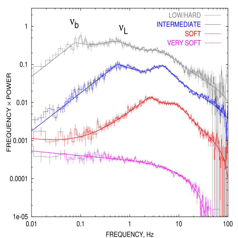
Figure 6: Power spectrum (PDS) evolution of the source from low/hard state (black) through intermediate state (blue) and soft state (red) to very soft state (purple). The break frequency $\nu_{b}$ and the low QPO frequency are clearly seen in low/hard, intermediate state and soft state. In the very soft state the power spectrum is featureless, no QPO and break are present. Any break and QPO features are washed out.

Figure 7: Upper panel: observed Fe K_α line equivalent width (EW) versus photon index $\Gamma$. EW increases toward the soft state. It is $\sim 150$ eV in the low/hard state and $\sim 1.3$ keV in soft and very soft states. Lower panel: inferred product of $\tau_{0}(Y+Y_{0})$ versus $\Gamma$.

Figure 8: Upper panel: The observed correlations between photon index $\Gamma$ and low frequency $\nu_{L}$ (orange points) which are compared with that in two other BHCs sources, XTE J1550-564 and GRS 1915+105. The saturation value of the index varies from source to source but it does not exceed the theoretically predicted value $2.8$ for the converging flow of non-relativistic temperature (see TZ98). Presumably, the saturation value of the index depends on the plasma temperature of the converging flow (LT99). Lower panel: The observed correlation between photon index $\Gamma$ and break frequency $\nu_{B}$ for Cyg X-1

Figure 10: Comptonization enhancement factor ${\cal E}_{\rm Comp}$ vs photon index $\Gamma$.

Figure 11: Observed ratio of the Comptonized photon flux $F_{comp}$ and the total photon flux $F_{comp}+F_{th}$ versus the photon index $\Gamma$. In the low/hard state the soft photon (disk) radiation is fully Comptonized in the hot electron environment. The ratio steadily decreases toward the soft state $\Gamma>2$. It is evident that the area of the Comptonized region (presumably converging flow) shrinks as a source undergoes the state transition.

Figure 12: Observed correlation of break frequency $\nu_{b}$ vs low frequency $\nu_{L}$ which is fitted by the broken power law (solid line). For high frequency values ($\nu_{L}>2.2$ Hz) the power-law index is approximately 1.65 as for the low ones that is approximately 1 (see text).

Figure 14: The inferred reflection scaling factor R as a function of the index using the MZ95 reflection model.

Figure 15: The variation of the photon index in Cyg X-1 throughout the entire RXTE mission.

Table 1: Summary of RXTE archive data on Cyg X-1

Proposal ID	Start Date	Stop Date	Time, sec	$N_{int}$	${\bar{N}_{PCUon}}$
10235-01	12/02/1996	17/02/1996	9332.18	4	5.0
10236-01	15/12/1996	18/12/1996	28239.78	13	5.0
10412-01	22/05/1996	12/08/1996	18125.03	9	4.94
10238-01	26/03/1996	03/02/1997	7475.19	3	3.65
10240-01	12/02/1996	19/12/1996	44813.12	16	4.56
10241-01	23/10/1996	24/10/1996	5088.0	2	4.37
10257-01	08/06/1996	12/07/1996	2432.0	4	5.0
10512-01	04/06/1996	18/06/1996	8012.22	6	5.00
20173-01	17/01/1997	20/01/1997	26883.84	8	5.0
20175-01	25/06/1997	02/01/1998	17783.69	7	4.99
30155-01	22/12/1998	28/12/1998	38003.49	16	4.81
30157-01	11/12/1997	09/12/1998	117347.25	47	4.85
30158-01	10/12/1997	30/12/1997	30587.26	11	4.90
30162-01	12/05/1998	10/10/1998	17892.08	7	5.00
40099-01	14/01/1999	11/02/2000	115199.16	64	3.73
40100-01	14/02/1998	02/14/2002	197798.51	90	3.82
40101-01	27/09/1999	10/10/1999	23505.19	19	3.93
40102-01	05/01/2000	10/01/2000	234309.48	84	3.09
40417-01	25/04/1999	13/06/1999	11004.28	8	2.92
50110-01	11/02/2000	06/04/2002	387571.88	210	3.22
50109-01	22/12/2000	15/02/2001	59020.71	40	3.90
50109-03	05/11/2000	10/01/2001	60428.65	22	3.64
50119-01	28/10/2000	04/01/2001	48984.88	23	3.82
60089-01	19/08/2001	30/08/2001	31545.51	13	2.80
60089-02	23/09/2001	28/10/2001	14409.54	6	3.11
60089-03	07/10/2001	21/02/2002	60380.83	24	3.15
60090-01	08/03/2002	03/04/2004	363880.25	189	2.88
60091-01	15/10/2001	22/10/2001	26984.65	12	3.85
60136-03	28/06/2001	09/07/2001	2512.0	5	3.12
70015-04	15/09/2002	17/09/2002	7685.78	3	3.68
70414-01	30/07/2002	29/12/2002	21393.17	14	4.12
80111-01	19/04/2003	20/04/2003	38834.50	13	3.30

Table 2: Results of fitting PCA/HEXTE spectrum with BMC model.

MODEL/PARAMETER aaaaaaaaaaaaaaaaa VALUE
aaaaaaaaaaaaaaaaLow/Hard State
BMC
aaaa$\Gamma$,aaaaaaaaaaaaaaaaaa.aaaaaaaaaaaaa $1.47\pm 0.01$
aaaa$kT_{col}$, keV .aaaaaaaaaaaaaaaaaaaaaaa $0.73_{-0.06}^{+0.04}$
aaaaA aaaaaaaaaaaaaaaaaaaaaaaaaaaaaaa $2.04\pm 0.06$
GAUSSIAN (6.4 keV fixed)
aaaa$\sigma$, aaaaaaaaaaaaaaaaaaaaaaaaaaaaaaa $0.71\pm 0.17$
aaaaEW, eVaaaaaaaaaaaaaaaaaaaaaaaaaa $198$
HIGHECUT
aaaa$E_{cut}$, keV aaaaaaaaaaaaaaaaaaaaaaaa $33.8_{-2.6}^{+3.6}$
aaaa$E_{fold}$, keV aaaaaaaaaaaaaaaaaaaaaaa $212\pm 13$
CONSTANT (Cross-Normalization)
aaaaPCA/HEXTE A aaaaaaaaaaaaaaaaaa $0.81\pm 0.01$
aaaaPCA/HEXTE B aaaaaaaaaaaaaaaaaa $0.81\pm 0.01$
aaaa$\chi^{2}_{\nu}\,(N_{dof})$ aaaaaaaaaaaaaaa.aaaaaaaaa 0.84 (159)
aaaaaaaaaaaaaaaaIntermediate State
BMC
aaaa$\Gamma$,aaaaaaaaaaaaaaaaaa.aaaaaaaaaaaaa $1.83\pm 0.01$
aaaa$kT_{col}$, keV .aaaaaaaaaaaaaaaaaaaaaaa $0.56\pm 0.02$
aaaaA aaaaaaaaaaaaaaaaaaaaaaaaaaaaaaa $1.08\pm 02$
GAUSSIAN (6.4 keV fixed)
aaaa$\sigma$, aaaaaaaaaaaaaaaaaaaaaaaaaaaaaaa $1.46\pm 0.09$
aaaaEW, eVaaaaaaaaaaaaaaaaaaaaaaaaaa $930$
HIGHECUT
aaaa$E_{cut}$, keV aaaaaaaaaaaaaaaaaaaaaaaa $31.2_{-1.8}^{+3.1}$
aaaa$E_{fold}$, keV aaaaaaaaaaaaaaaaaaaaaaa $181\pm 12$
CONSTANT (Cross-Normalization)
aaaaPCA/HEXTE A aaaaaaaaaaaaaaaaaa $0.86\pm 0.01$
aaaaPCA/HEXTE B aaaaaaaaaaaaaaaaaa $0.85\pm 0.01$
aaaa$\chi^{2}_{\nu}\,(N_{dof})$ aaaaaaaaaaaaaaa.aaaaaaaaa 0.90 (159)
aaaaaaaaaaaaaaaaVery Soft State
BMC
aaaa$\Gamma$,aaaaaaaaaaaaaaaaaa.aaaaaaaaaaaaa $2.64\pm 0.02$
aaaa$kT_{col}$, keV .aaaaaaaaaaaaaaaaaaaaaaa $0.51\pm 0.02$
aaaaA aaaaaaaaaaaaaaaaaaaaaaaaaaaaaaa $0.66\pm 0.02$
GAUSSIAN (6.4 keV fixed)
aaaa$\sigma$, aaaaaaaaaaaaaaaaaaaaaaaaaaaaaaa $1.33\pm 0.06$
aaaaEW, eVaaaaaaaaaaaaaaaaaaaaaaaaaa $1366$
HIGHECUT
aaaa$E_{cut}$, keV aaaaaaaaaaaaaaaaaaaaaaaa $26.7_{-5.1}^{+6.0}$
aaaa$E_{fold}$, keV aaaaaaaaaaaaaaaaaaaaaaa $149^{+138}_{-51}$
CONSTANT (Cross-Normalization)
aaaaPCA/HEXTE A aaaaaaaaaaaaaaaaaa $0.91\pm 0.03$
aaaaPCA/HEXTE B aaaaaaaaaaaaaaaaaa $0.88\pm 0.03$
aaaa$\chi^{2}_{\nu}\,(N_{dof})$ aaaaaaaaaaaaaaa.aaaaaaaaa 1.16 (159)

References

- Abramovitz & Stegun (1970) Abramowitz, M., & Stegun, I. 1970, Handbook of Mathematical Functions, Dover Publications, New York
- Aharonian et al. (2005) Aharonian, F. M. et al. 2005, Science, 309, 736
- Axelsson, Borgonovo & Larsson (2005) Axelsson, M., Borgonovo, L. & Larsson, S. 2005, A&A, 438, 999
- Bambynek et al. (1972) Bambynek, W. et al. 1972, Rev. Mod. Phys., 44, 716
- Barr et al. (1985) Barr, P., White, N.E., & Page, C.G. 1985, MNRAS, 216, P65
- Basko (1978) Basko, M. M. 1978, ApJ, 223, 296
- Basko, Sunyaev & Titarchuk (1974) Basko, M. M., Sunyaev, R.A. & Titarchuk, L.G. 1974, A&A, 31, 249
- Belloni (2005) Belloni, T. 2005, astro-ph/0507556
- Borozdin et al. (1999) Borozdin, K., Revnivtsev, M., Trudolyubov, S., Shrader, C, & Titarchuk, L. 1999, ApJ, 517, 367 (BRT99)
- Chakrabarti & Titarchuk (1995) Chakrabarti S.K. & Titarchuk, L. G. 1995, ApJ, 455, 623
- Cui et al. (1998) Cui, W., Ebisawa, K., Dotani, T. & Kubota, A.. 1998, ApJ, 493, L75
- Cui et al. (1997) Cui, W., Zhang, S.N., Focke, W. & Swank, J.H. 1997, ApJ, 484, 383
- Dewangan, Titarchuk, & Griffiths (2006) Dewangan, G. Titarchuk, L., & Griffiths, R.E. 2006, ApJ, 637, L21
- Di Salvo et al. (2001) Di Salvo T., Done, C., Zycki, P.T., Burderi, L., & Robba, N.R. 2001, ApJ, 547, 1024
- Ebisawa et al. (1996) Ebisawa, K., et al. 1996, ApJ, 467, 419
- Esin et al. (1998) Esin, A. A.; Narayan, R., Cui, W., Grove, J. E., Zhang, S.-N. 1998, ApJ, 505, 854
- Farinelli et al. (2005) Farinelli, R., et al. 2005, A&A, 434, 25
- Frontera et al. (2001) Frontera, F., et al. 2001, ApJ, 546, 1027
- George & Fabian et al. (1991) George, I., & Fabian, A.C. 1991, MNRAS, 249, 352
- Gies et al. (2003) Gies, D.R. et al. 2003, ApJ, 583, 424
- Gilfanov & Aref’ev (2005) Gilfanov, M., & Arefiev, V. 2005, MNRAS, accepted, (astro-ph/0501215)
- Gilfanov, Churazov & Revnivtsev (1999) Gilfanov, M., & Churazov, E. & Revnivtsev, M. 1999, A&A, 352, 182 (GCR99)
- Grove et al. (1998) Grove, J.E., et al. 1998, ApJ, 500, 899
- Herrero et al. (1995) Herrero, J., et al. 1995, A&A, 297, 556
- Kallman et al. (2004) Kallman, T.R., Palmeri, P., Bautista, M.A., Mendoza, C. & Krolik, J.H. 2004, ApJS, 155, 675
- Kaper (1998) Kaper, L. 1997, in ASP Conf. Ser. 131, Boulder-Munich II: Properties of Hot, Luminous Stars, ed. I.D. Howard (San Francisco: ASP), 427
- Klein-Wolt et al. (2002) Klein-Wolt, M., et al. 2002, MNRAS, 331, 745
- Laming & Titarchuk (2004) Laming, J.M. & Titarchuk, L. 2005, ApJ, 615, L121 (LaT04)
- Lapidus, Sunyaev & Titarchuk (1985) Lapidus, I.I., Sunyaev, R.A. & Titarchuk, L. 1985, Astrofizika (Astrophysics), 23, 515
- Laurent & Titarchuk (1999) Laurent, P. & Titarchuk, L. 1999, ApJ, 511, 289 (LT99)
- Laurent & Titarchuk (2001) Laurent, P. & Titarchuk, L. 2001, ApJ, 562, L67
- Magdziarz & Zdziarski (1995) Magdziarz, P., & Zdziarski, A.A. 1995, MNRAS, 273, 837 (MZ95)
- Makishima et al. (1986) Makishima, K et al. 1986, ApJ, 308, 635
- McClintock & Remillard (2004) McClintock & Remillard, R. 2004, preprint (astro-ph/0306213)
- McConnell et al. (2002) McConnell, M.L., et al. 2002, ApJ, 572,984
- McConnell et al. (2002) McHardy, I. M., Gunn, K. F., Uttley, P., & Goad, M.R. 2005, MNRAS, 359, 1469
- Miller & Homan (2005) Miller, J.M., & Homan, J. 2005, ApJ, 618, 107
- Niedzwieski & Zdziarski (2005) Niedzwieski, A. & Zdziarski, A. A. 2005, MNRAS in press, astro-ph/0507579
- Petterson (1978) Petterson, K. 1978, ApJ, 224, 625
- Pottschmidt et al. (2003) Pottschmidt, K., et al. 2003, A&A, 407, 1039 (P03)
- Proga (2005) Proga, D. 2005, ApJ, 630, L9
- Proga & Kallman (2004) Proga, D. & Kallman, T.R. 2004, ApJ, 616, 688
- Sunyaev & Titarchuk (1985) Sunyaev, R.A. & Titarchuk, L.G. 1985, A&A, 143, 374
- Sunyaev & Titarchuk (1980) Sunyaev, R.A. & Titarchuk, L.G. 1980, A&A, 86, 121 (ST80)
- Titarchuk (1994) Titarchuk, L.G. 1994, ApJ, 434, 570
- Titarchuk (1987) Titarchuk, L.G. 1987, Astrofizika (Astrophysics), 26, 98
- Titarchuk et al. (2002) Titarchuk, L.G., Cui, W., & Wood, K.S., 2002, ApJ, 576, L49