Molecular Gas in the Low Metallicity, Star Forming Dwarf IC 10

Abstract

We present a complete survey of CO ($1\rightarrow 0$) emission in the Local Group dwarf irregular IC 10. The survey, conducted with the BIMA interferometer, covers the stellar disk and a large fraction of the extended H I envelope with the sensitivity and resolution necessary to detect individual giant molecular clouds (GMCs) at the distance of IC 10 (950 kpc). We find 16 clouds with a total CO luminosity of $1\times 10^{6}$ K km s^-1 pc², equivalent to $4\times 10^{6}$ M_⊙ of molecular gas using the Galactic CO-to-H₂ conversion factor. Observations with the ARO 12m find that BIMA may resolve out as much as 50% of the CO emission, and we estimate the total CO luminosity as $\sim 2.2\times 10^{6}$ K km s^-1 pc². We measure the properties of 14 GMCs from high resolution OVRO data. These clouds are very similar to Galactic GMCs in their sizes, line widths, luminosities, and CO-to-H₂ conversion factors despite the low metallicity of IC 10 ($Z\approx 1/5Z_{\odot}$). Comparing the BIMA survey to the atomic gas and stellar content of IC 10 we find that most of the CO emission is coincident with high surface density H I. IC 10 displays a much higher star formation rate per unit molecular (H₂) or total ($\mbox{\rm{H~{}I}}+\mbox{\rm H${}_{2}$}$) gas than most galaxies. This could be a real difference or may be an evolutionary effect — the star formation rate may have been higher in the recent past.

1. Introduction

Star forming dwarf galaxies tend to have low metallicities, intense interstellar radiation fields, and shallow potential wells. For these reasons, dwarfs are often used as astrophysical laboratories in which to study the effect of extreme conditions on the interstellar medium (ISM) and star formation. The similarity between local dwarf galaxies and the first star forming systems — which were also low mass and chemically primitive — further motivates such studies. Unfortunately, the smallest actively star forming systems are not very luminous and are therefore difficult to observe at any significant distance. Systems the size of the Large Magellanic Cloud (LMC) may be studied in some detail out to 10 Mpc or more, but detailed observations of smaller systems are possible only in the Local Group. In practice this limits such studies to a handful of systems, the Local Group irregular galaxy IC 10, the Small Magellanic Cloud (SMC), NGC 6822, and perhaps a few other Local Group dwarfs (Mateo, 1998).

In this paper we present a new study of the molecular gas component of IC 10. We have conducted a complete survey of ¹²CO ($1\rightarrow 0$) emission from IC 10 using the BIMA interferometer. This survey covers the optical disk and much of the extended H I structure surrounding IC 10 with the resolution and sensitivity necessary to detect individual giant molecular clouds (GMCs). We also present new single dish observations towards most of the CO emission from IC 10 using the ARO 12m and we measure macroscopic properties of $14$ GMCs using the high-resolution OVRO observations by Walter (2003). We combine these data with literature observations of IC 10 at several wavelengths to address three questions: 1) How do the GMCs in IC 10 compare to the GMCs found in Local Group spirals? 2) Can we predict the molecular gas content from the hydrostatic pressure? 3) Do stars form out of molecular gas at the same rate in IC 10 as in spiral galaxies?

There are several reasons to expect the relationship between atomic gas, molecular gas, and star formation in IC 10 might be different from that in spiral galaxies. Dust plays a crucial role in setting the abundance of molecular gas by shielding molecular gas from dissociating radiation and serving as the site of molecular hydrogen formation. With its low metallicity ($Z_{IC~{}10}\approx 1/5~{}Z_{\odot}$, Garnett, 1990), IC 10 might be expected to have to have a low dust-to-gas ratio. The interstellar radiation field (ISRF) in IC 10 should also be more intense than in most spiral galaxies due to the high star formation rate, low dust abundance (lower extinction), and low metallicity (less line blanketing). A more intense ISRF will dissociate molecular hydrogen faster and perhaps inhibit the formation of H₂ by heating the grain surfaces. It may also affect different molecular species differently as, for example, H₂ self-shields while CO is dissociated. Other factors, for instance the lack of shear (perhaps diminishing rotational support against GMC collapse), the absence of spiral density waves (the sites of GMC formation in spirals), and the simple underabundance of carbon and oxygen (and thus, presumably, of CO to trace and cool molecular gas), further distinguish IC 10 from the Galactic environment.

This paper is organized in the following way. In §2 we summarize the macroscopic properties of IC 10 and present maps of several components of the galaxy. We emphasize the similarity of IC 10 to the SMC in gross properties and discuss IC 10’s vigorous present day star formation. In §3 we present our BIMA and ARO 12m observations, discuss how we identified signal in the survey, describe our algorithm for measuring GMC properties, and note several other datasets used in this paper. In §4 we present the results of the BIMA survey and our GMC property measurements. In §5 we present our analysis of the molecular content in IC 10. We emphasize the surprising similarity between IC 10 clouds and GMCs in large spiral galaxies. We examine quantitative relationships between atomic gas, molecular gas, and star formation. We consider the hypothesis that the hydrostatic pressure predicts the molecular to atomic gas ratio and look at the efficiency with which molecular gas forms stars in IC 10. In §6, we summarize our findings and suggest some future avenues of investigation in IC 10.

2. Description of IC 10

Along with the SMC, IC 10 is the best example of a low-mass, metal-poor, actively star-forming galaxy in the Local Group. Table 1 summarizes a number of properties of IC 10. IC 10 has stellar, atomic gas, and dynamical masses of $\sim 4,~{}2,~{}\mbox{and}~{}15\times 10^{8}$ M_⊙, respectively (Jarrett et al., 2003; Huchtmeier & Richter, 1988; Mateo, 1998); by comparison, the SMC has stellar, atomic gas, and dynamical masses of $\sim 4,~{}4,~{}\mbox{and}~{}24\times 10^{8}$ M_⊙ (Stanimirović, Staveley-Smith, & Jones, 2004). IC 10 has a metallicity of 12 + log O/H $\approx 8.25$ (Lequeux et al., 1979; Garnett, 1990), intermediate between the SMC and the LMC ($8.0$ and $8.4$, respectively, Dufour, 1984). Like the SMC, IC 10 has irregular morphology, ongoing high mass star formation, and an extended H I envelope. IC 10 is probably associated with M 31 but the separation between the two galaxies is fairly large. At our adopted distance ($950$ kpc), IC 10 is separated from M 31 galaxy by $\gtrsim 250$ kpc. Another close cousin to IC 10 exists just beyond the Local Group — the post starburst dwarf NGC 1569 at a distance of $\sim 2$ Mpc. That galaxy is also relatively isolated, with atomic gas and total masses of $\sim 1$ and $\sim 3\times 10^{8}$ (Israel, 1988), respectively, and a metallicity of $\sim 1/4~{}Z_{\odot}$ (Calzetti et al., 1994).

IC 10 has a higher star formation rate (SFR) than the SMC, though the exact SFR is somewhat uncertain. The H$\alpha$ flux implies a SFR of $\sim 0.2$ M_⊙ yr^-1 with a standard correction for internal extinction, but this value may be as high $0.6$ M_⊙ yr^-1 if the larger extinction estimates in the literature are correct (Gil de Paz et al., 2003; Yang & Skillman, 1993; Borissova et al., 2000). By comparison, Wilke et al. (2004) estimates an SFR of $\sim 0.05$ M_⊙ yr^-1 in the SMC (with the FIR and H$\alpha$ in agreement after corrections for extinction and absorption). Massey & Holmes (2002), Crowther et al. (2003), and others have noted IC 10’s prodigious content of Wolf Rayet (WR) stars. More than $30$ have been spectroscopically confirmed (Crowther et al., 2003) and Massey & Holmes (2002) estimate from photometry that the total number may be $\sim 100$. By contrast, the SMC contains only $12$ WR stars (Massey et al., 2003). The number of WR stars in a galaxy should provide a distance independent estimate of the high mass stellar content (and thus formation rate). Thus H$\alpha$ and WR star counts suggest IC 10 to have a star formation rate $3$ – $4$ times that of the SMC. Measurements of internal extinction (Yang & Skillman, 1993; Borissova et al., 2000) and the higher number of WR stars estimated by Massey & Holmes (2002) suggest the SFR may easily be as high as $\sim 0.5$ M_⊙ yr^-1. We note that the FIR and radio continuum yield SFR estimates considerably lower ($\sim 0.05$ M_⊙ yr^-1 Thronson et al., 1990; White & Becker, 1992; Bell, 2003) perhaps as a result of a higher UV escape fraction or lower dust abundance.

The unusually high content of WR stars has led to claims that IC 10 is the nearest starburst galaxy — the surface density of WR stars is the highest of any local group galaxy and the average across the entire galaxy is comparable to the most actively star forming regions in M 33 (Massey & Armandroff, 1995). The disrupted morphology of the H I distribution also suggests a violent recent history. The H I distribution across the disk of the galaxy is characterized by seven large holes, possibly carved out by winds or supernovae (Wilcots & Miller, 1998). The central regions of these holes are free of H I emission down the to a sensitivity limit of $1\times 10^{19}$ cm^-2 (3$\sigma$), equivalent to about $0.1$ M_⊙ pc^-2. IC 10 has a substantial molecular gas content compared to other galaxies of its size, suggesting that the period of vigorous star formation may be ongoing. IC 10’s CO luminosity of $\sim 2\times 10^{6}$ K km s^-1 pc² is an order of magnitude higher than that of the SMC ($\sim 8\times 10^{4}$ K km s^-1 pc², Mizuno et al., 2001) or NGC 1569 ($\sim 10^{5}$ K km s^-1 pc², Greve et al., 1996; Taylor et al., 1999). Indeed, Wilcots & Miller (1998) calculated only $\sim 7$ – $21$ supernovae would be needed to create all of dramatic holes in the H I distribution; thus, based on the observed number of WR stars — possibly as high as 100 and each representing a future supernova — IC 10 may have only experienced a small fraction of the Type II supernovae in store for it in the near future. This would seem to place IC 10 in contrast to the comparatively quiescent SMC and the post starburst NGC 1569 (where a burst of star formation may have ended as recently at 5 Myr ago Greggio et al., 1998).

Figures 1 and 2 show maps of the atomic gas content, stellar surface density, and H$\alpha$ surface brightness in IC 10, with the positions of spectroscopically confirmed WR stars (Crowther et al., 2003) noted in Figure 2 (the larger, $\sim 100$, number of WR stars from Massey & Holmes, 2002, await spectroscopic confirmation and publication of their locations). The complex H I structure is described by Wilcots & Miller (1998) in the following way: the stellar disk lies within a larger H I disk which shows rotation aligned with the stellar disk, the whole galaxy lies within a much more extended H I structure that is counter-rotating and complex. The H I disk extends beyond the stars to the east of the galaxy and forms part of a contiguous position-velocity structure with the extended H I envelope to the south and east of the galaxy. This large envelope may be have recently interacted with the galaxy in a way that triggered the present star formation in the galaxy. Most of the star formation lies in the central part of the disk, where a large H I cloud is the site of much of the ongoing star formation activity. The dramatic holes that give the disk its disturbed (almost spiral) morphology are probably a result of stellar winds or perhaps supernovae.

Because it lies close to the Galactic plane ($b=-3.3$), the distance to IC 10 remains uncertain. Current estimates of the distance range from a lower limit of $500$ kpc (Sakai et al., 1999) to $950$ kpc (Hunter, 2001). In this paper, we adopt $950$ kpc, the distance obtained by Hunter (2001) using the tip of the red giant branch and a reddening confirmed by comparison with color magnitude diagrams. The resulting distance is close to $1$ Mpc, a value frequently adopted in the literature, making for easy comparison. The values presented in Table 1 and the results of this paper have been scaled to this distance of $950$ kpc.

Table 1 Properties of IC 10

Property	Value	Reference
Hubble Type	dIrr	Mateo (1998)
Distance	950 kpc	Hunter (2001)
Axis Ratio	0.67	Jarrett et al. (2003)
Dynamical Mass	$\sim 1.7\times 10^{9}$ M⊙	Mateo (1998)
Absolute B Magnitude	$-16.3$	Gil de Paz et al. (2003)
Stellar Mass	$4\times 10^{8}$ M⊙	Jarrett et al. (2003)
H I Mass	$2\times 10^{8}$ M⊙	Huchtmeier & Richter (1988)
H$\alpha$ Luminosity	$1\times 10^{40}$ erg s-1	Gil de Paz et al. (2003); Thronson et al. (1990)
FIR Luminosity	$5\times 10^{7}$ L⊙	Melisse & Israel (1994)
1.4 GHz Luminosity	$3.4\times 10^{19}$ W Hz-1	White & Becker (1992)
Metallicity	log O/H + 12 = 8.25	Lequeux et al. (1979); Garnett (1990)
SFRHα	$0.2$ M⊙ yr-1	Gil de Paz et al. (2003); Kennicutt et al. (1994)
SFRFIR	$0.05$ M⊙ yr-1	Melisse & Israel (1994); Bell (2003)
SFR${}_{1.4~{}GHz}$	$0.07$ M⊙ yr-1	White & Becker (1992); Bell (2003)
$\Sigma_{SFR}$	$0.1$ M⊙ yr-1 kpc-2
CO Luminosity		this work (§4.2)
Best Estimate	$2.2\times 10^{6}$ K km s-1 pc2
Lower Limit	$1.6\times 10^{6}$ K km s-1 pc2
Upper Limit	$2.8\times 10^{6}$ K km s-1 pc2

3. Observations

In this paper we present two new datasets: a complete survey of the disk of IC 10 obtained with the BIMA interferometer (described by Welch et al., 1996), and single-dish pointed observations obtained with the Arizona Radio Observatory (ARO) 12m to check for emission missed by the BIMA survey. In this section we describe the acquisition and reduction of both data sets and the algorithm we used to identify signal in the BIMA survey. We also introduce several previously published data sets that we use in our analysis and summarize our algorithm for measuring GMC properties.

3.1. The BIMA Survey

The BIMA survey was conducted in the most compact BIMA configuration, the D array, and has a resolution of $14\arcsec$. The survey took place over the course of four observing seasons: fall 2000, spring 2001, fall 2001, and spring 2002. We observed IC 10 during 34 tracks ranging from 2 to 13 hours in length for a total of $250$ hours of observing time. For most tracks, we also observed a planet once or twice to check the absolute flux of the phase calibrator. Each track consisted of $\sim 20$ fields arranged on a hexagonal grid with pointing centers spaced by $78^{\prime\prime}$ (BIMA has a $\approx 100\arcsec$ half-power field of view at 115.27 GHz). The correlator configuration varied somewhat over the survey (the central velocity and channel width changed slightly) but a typical setup covered a bandwidth of 100 MHz ($\approx 260$ km s^-1) near the velocity of IC 10 with a velocity resolution of $\approx 1$ km s^-1. The final survey has a resolution of 3 km s^-1 across a 150 km s^-1 bandwidth near the velocity of IC 10, so these variations in the correlator setup do not affect the final data. For the survey $1$ K = $2.04$ Jy beam ^-1.

We reduced the observations using the MIRIAD software package . We corrected the observations of the phase calibrator and the source for line length variations (BIMA monitors the electronic path length to each antenna by periodically sending a signal to the antenna and back and measuring the phase on return, allowing variations to be removed from the data during reduction). We flagged data with shadowing or very high amplitudes, and channels at the edge of the correlator. We adopted the flux for the phase calibrator shown in Table 2 and self-calibrated on it, assuming that the phase calibrator was unresolved by our $14^{\prime\prime}$ beam (we see no evidence of extended structure in our data). We transfered the gains and phases as a function of time to the source.

We combined the $(u,v)$ data from all 34 tracks, applied a natural weighting scheme, and inverted them into a spectral line map with velocity channels $3$ km s^-1 wide. We applied a CLEAN algorithm to each plane of the data cube in order to remove artifacts generated by incomplete $(u,v)$ coverage. We capped the algorithm at $500$ iterations in each map and did not clean sources less than $2\sigma$ in peak brightness. The final maps cover an 75 square arcminutes at better than 0.2 K sensitivity with an angular resolution of $14\arcsec$, a velocity resolution of $3$ km s^-1, and a velocity coverage spanning LSR velocities from $-400$ km s^-1 to $-250$ km s^-1.

The flux of our phase calibrator, 0102+584, varied by a factor of 3 over the two year duration of the survey, and as a result, the amplitude calibration of the survey may be somewhat uncertain. We used values interpolated from the BIMA calibrator monitoring campaign, adjusted by as much as $30\%$ based on comparisons between 0102+584 and planets in our own observations. Based on the variation of the phase calibrator and the scatter within the planet/phase calibrator fluxes within our own data, we estimate that the flux calibration of the survey is uncertain by $30\%$. These gain errors may be nonuniform across the survey because different tracks contribute to different parts of the map.

Table 2 The BIMA Survey

Observing Season	Flux of Calibrator	Dates of Tracks (Duration in Hours)
Fall 2000 (45h)	2.5 Jy	11 Oct (10), 12 Oct (12), 16 Oct (10), 22 Oct (13)
Spring 2001 (75h)	1.3 Jy	7 Jun (10), 10 Jun (10), 12 Jun (11), 16 Jun (10),
		17 Jun (10), 21 Jun (5), 23 Jun (4), 29 Jun (4),
		1 Jul (3), 3 Jul (8)
Fall 2001 (83h)	2.0 Jy	23 Sep (7), 26 Sep (13), 28 Sep (6), 2 Oct (6),
		3 Oct (11), 6 Oct (5), 7 Oct (5), 12 Oct (8),
		13 Oct (5), 20 Oct (8), 21 Oct (9)
Spring 2002 (71h)	3.0 Jy	25 May (8), 26 May (10), 27 May (5), 28 May (8),
		29 May (3), 31 May (8), 6 Jun (9), 8 Jun (2),
		13 Jun (7), 15 Jun (5), 16 Jun (6)

3.1.1 Sensitivity of the Survey

On average, $50\%$ of the time in a given track was spent integrating on IC 10. The remainder of the time was spent on calibration and slewing. The $250$ hours of observing time used for the survey translates into $\approx 125$ hours of integration on source. The total area targeted was $13\arcmin\times 8\arcmin\approx 100$ square arcminutes. This corresponds to an integration time per pointing of $\sim 2$ hours. The theoretical $1\sigma$ noise for $2$ hours of observation with the D array at $3$ km s^-1 velocity resolution and our typical system temperature ($500$ K) is $\sim 0.05$ K. Figure 3 shows a map of the sensitivity of the survey, measured from the RMS variation in the signal-free channels at the edges of the map, which is somewhat higher than the estimate above due to missing antennas, atmospheric decorrelation, and other inefficiencies. About $40$ square arcminutes of our survey have a $1\sigma$ sensitivity better than $0.1$ K, another $35$ square arcminutes have $1\sigma$ sensitivities between $0.1$ and $0.2$ K. Thus the final survey covers $75$ square arcminutes at better than $0.2$ K sensitivity. The noise in the survey is quite Gaussian. We find $15.9\%$, $2.3\%$, and $0.13\%$ of the emission in the final cube to lie below $-1\sigma$, $-2\sigma$, and $-3\sigma$, respectively, almost exactly what would be expected from a normal distribution.

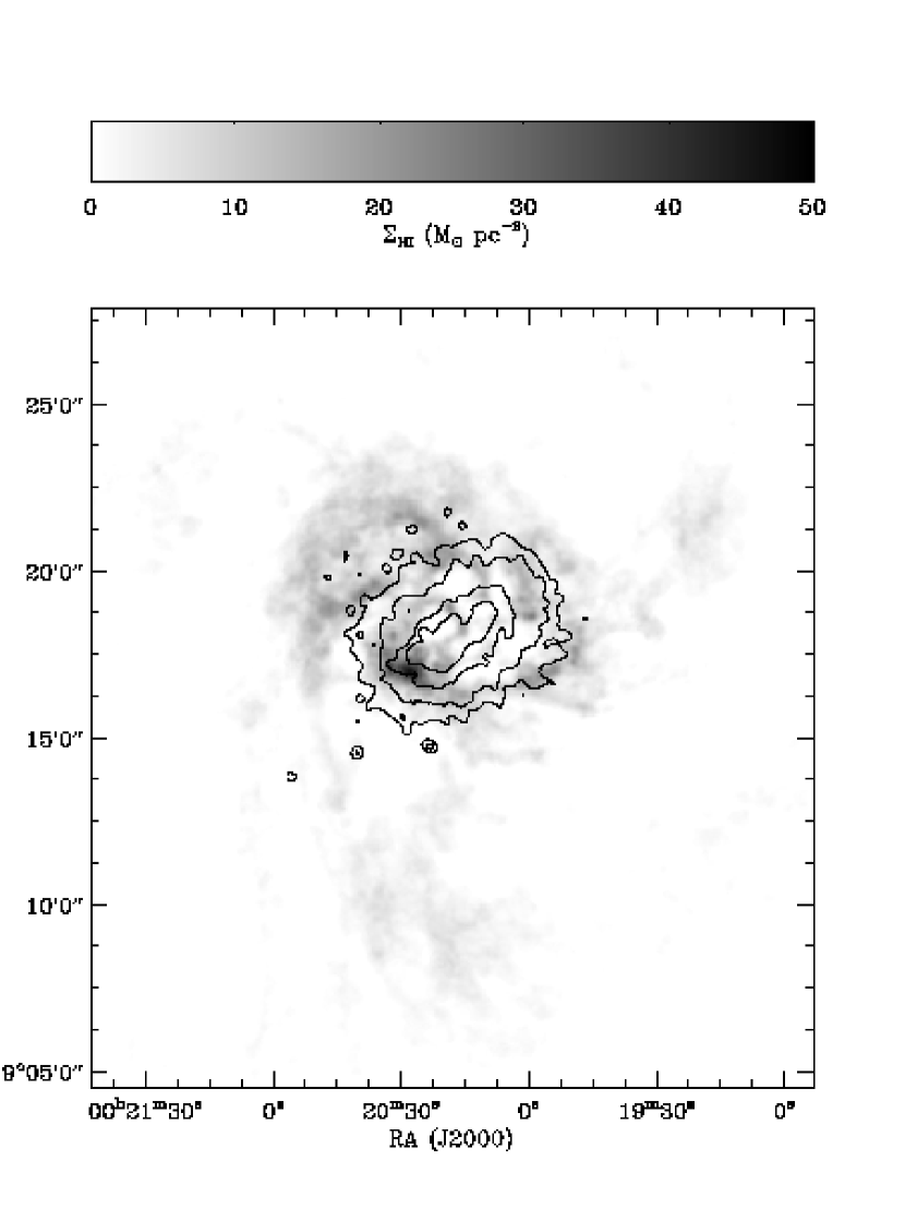
Figure 1.— H I emission from IC 10 (grayscale, Wilcots & Miller, 1998) with stellar surface density contours overlaid (black, derived from $K$-band data from Jarrett et al., 2003). The stellar surface density contours are at 50, 100, 200, and 300 M_⊙ pc^-2. The H I distribution extends well beyond the optical disk, stretching for more than $20$ arcminutes ($>5.5$ kpc). H I contours show surface densities of 1, 10, 20, and 30 M_⊙ pc^-2. The surface densities shown are line of sight surface densities, with no correction for inclination.

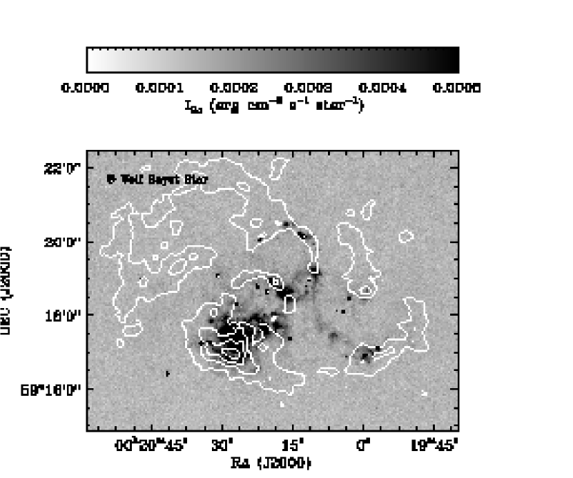
Figure 2.— H$\alpha$ emission from IC 10 (Gil de Paz et al., 2003) with H I contours (10, 20, and 30 M_⊙ pc^-2, Wilcots & Miller, 1998) overplotted. The locations of spectroscopically confirmed WR stars (Crowther et al., 2003) are shown for comparison.

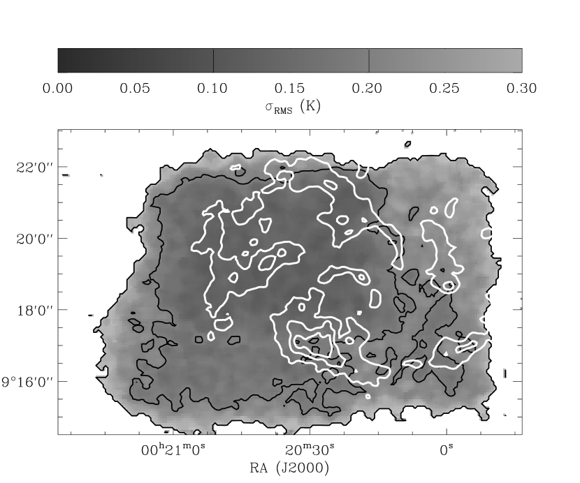
Figure 3.— Sensitivity of the BIMA D-array survey in Kelvin. The white contours show H I surface density (10, 20, and 30 M_⊙ pc^-2, Wilcots & Miller, 1998). The black contours show sensitivities of 0.3 and 0.6 K km s^-1 per 3 km s^-1 channel.

3.1.2 Signal Identification in the Survey

We identified signal using the statistic of merit equal to the the product of the probability of generating the observed signal or higher in each of five adjacent velocity channels along a line of sight (referred to by the subscripts $1$ to $5$) from Gaussian noise. This statistic, $X$, is calculated via the formula

$$X=P(\frac{I_{1}}{\sigma})\times P(\frac{I_{2}}{\sigma})\times P(\frac{I_{3}}{\sigma})\times P(\frac{I_{4}}{\sigma})\times P(\frac{I_{5}}{\sigma})$$ (1)

where $P(\frac{I_{i}}{\sigma})$ is the probability of generating an intensity equal to or greater than $I_{i}$ from a distribution of normally distributed noise with standard deviation $\sigma$. For Gaussian noise, $P(\frac{I_{i}}{\sigma})$ is given by

$$P(\frac{I_{i}}{\sigma})=\left\{\begin{array}[]{ll}\frac{1}{2}\left[1-\mbox{erf}\left(\frac{I_{i}}{\sqrt{2}\sigma}\right)\right]&\left(I_{i}>0\right)\\ \\ 1&\left(I_{i}\leq 0\right)\\ \end{array}\right.\mbox{ .}$$ (2)

The factor of $\frac{1}{2}$ results from normalizing the error function so that $\mbox{erf}\left(\infty\right)=1$ (rather than $\frac{1}{2}$). We consider all negative intensities to be the result of noise and so assign those data a $P(\frac{I_{i}}{\sigma})$ of 1. Therefore negative intensities can never contribute to a detection (which are identified by their low values of $X$).

We used this statistic to identify lines of sight with significant emission in the BIMA survey. We calculated $X$ for all combinations of 5 adjacent velocity channels in the survey. We then select all regions with $X\leq 10^{-9}$ and RMS sensitivity of $0.2$ K or better. This value of $X$ corresponds to $\approx 2\sigma$ emission across 5 channels, a single channel containing $\approx 6\sigma$ emission, or a range of intermediate cases. We chose this value, $X\leq 10^{-9}$, so that we do not expect a false detection over the BIMA survey. We checked our expected false positive rate by applying this algorithm to the negative part of the data set (which should consist only of noise). The algorithm identifies no significant emission in the negative part of the data cube.

We constructed a mask from the signal we identified. The mask is a set of flags (ones and zeros) that identifies regions of significant emission in the data cube (a 1 for a region containing emission, a 0 for a signal free region). In the analysis below we use the emission measured in the BIMA survey multiplied by the mask, so that signal free regions are treated as having zero emission while the data is used in regions containing significant signal. To be included in the mask, we required that region of the survey to have $X\leq 10^{-9}$ across most of a beam (at least three adjacent quarter-beam-sized pixels). In order to ensure that we did not miss extended, low-lying emission around the CO peaks, we included all regions within three velocity channels (a typical cloud line width) and one and a half beams of each significant region. As a result, the mask contains some noise at the edge but it is less likely to miss extended emission. The integrated intensity from the survey multiplied by the mask is shown in Figure 4.

This method does not produce a single point source sensitivity, but in worst case — $5$ channels at $2\sigma$ significance in the region of $0.2$ K sensitivity — we find all emission with an integrated intensity above 6 K km s^-1. This corresponds to $1.4\times 10^{5}$ M_⊙ over a BIMA synthesized beam at a Galactic CO-to-H₂ conversion factor (appropriate for the IC 10 GMCs but perhaps not for the diffuse gas). We detect emission with narrow line widths in high sensitivity regions down to even smaller luminosities, corresponding to masses of $\lesssim 10^{5}$ M_⊙ ($1.8$ K km s^-1, or $4\times 10^{4}$ M_⊙ over a BIMA beam, in the best case). A typical sensitivity over the whole survey is therefore $10^{5}$ M_⊙.

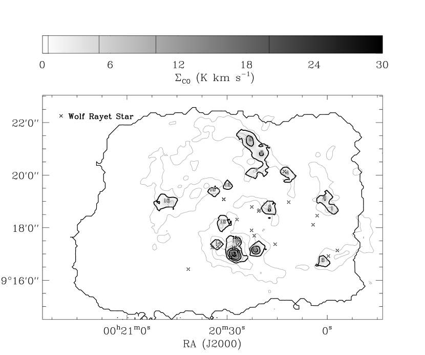
Figure 4.— The integrated intensity map resulting from the BIMA D array survey (grayscale). Black contours show the 1, 10, 20, and 30 K km s^-1 surface brightness contours. Numbers indicate the corresponding entry in Table 4. Light contours indicate H I column densities of 10, 20, and 30 M_⊙ pc^-2 (Wilcots & Miller, 1998) and the locations of spectroscopically confirmed WR stars are indicated (Crowther et al., 2003). CO emission is almost exclusively found along lines of sight with $\Sigma_{HI}>10$  M_⊙ pc^-2 ($N(\mbox{\rm{H~{}I}})=1.25\times 10^{21}$ cm^-2).

3.2. ARO 12m Observations

We observed 22 pointings in IC 10 with the Arizona Radio Observatory (ARO) 12m telescope at Kitt Peak. This telescope has a $55\arcsec$ ($\approx 250$ pc) half-power beam-width at 115.27 GHz. The data were acquired during an observing run in 2002 May 8–16. The locations of the ARO 12m pointings are listed in Table 3 and plotted along with the results of the BIMA survey and the H I contours in Figure 5 — though note that four of the pointings lie outside the map. The ARO 12m pointings were selected for two reasons. First, they were intended to check the flux measurements and line widths of the BIMA survey — especially to search for the presence of extended emission that might be resolved out by the interferometer. Second, they were selected to provide an independent search for CO emission at several points of interest not detected by BIMA — including H I peaks in the extended emission (possible locations of CO beyond the optical disk) and two of the H I holes identified by Wilcots & Miller (1998).

We observed both polarizations either with the 1 MHz filter banks or with the millimeter autocorrelator. We observed most pointings for about one hour, though several pointings were bright enough to be detected in only $\sim 30$ minutes. We position switched every six minutes, with the reference position separated from the pointing by 3 arcminutes in azimuth. In only one case, pointing 14, do we find evidence of emission in the reference positions close to the velocity of IC 10. Every six hours, after sunset, and after sunrise, a planet or other strong continuum source was observed to optimize the pointing and focus of the telescope. The median system temperature was 345 K.

We reduced the spectrum for each six-minute scan in the following manner. We removed noise spikes and bad channels by flagging all channels in each six minute scan with absolute values above the $5\sigma$ level (none of our sources were nearly this bright in a single scan). Several channels were known to be bad a priori and we flagged these as well. We then subtracted a linear baseline from the spectrum and binned it to a resolution of $\sim 4$ km s^-1. Finally, we averaged both polarizations and all scans to produce the final spectrum for each position.

The results of the ARO 12m pointings are summarized in Table 3. For spectra with detected signal we quote the peak temperature and the central velocity, velocity width, and integrated intensity from a three parameter Gaussian fit. For spectra without detections we quote a $3\sigma$ upper limit to the integrated intensity assuming a source $15$ km s^-1 wide (a typical FWHM line width for our detections). For spectra with detected emission, we also quote the results from the BIMA and OVRO data convolved to the resolution of the ARO 12m. We discuss the results of the comparison among the three datasets in Section 4.1. The final column indicates the BIMA survey clouds associated with each pointing.

Table 3 ARO 12M Results

Pointing	Telescope	$\alpha$	$\delta$	$1\sigma$ Noise	$T_{peak}$	$v_{ctr}$	$\sigma_{v}$	$I_{int}$	Clouds
		(J2000)	(J2000)	(mK)	(K)	(km s-1)	(km s-1)	(K km s-1)	Overlapped
1	ARO 12m	00 20 46.4	59 18 59.9	$20$	$0.10$	$-335.7$	$8.2$	$1.7$	B16
1	BIMA				$0.04$	$-332.4$	$4.2$	$0.4$
1	OVRO				$0.03$	$-332.0$	$3.0$	$0.2$
2	ARO 12m	00 20 22.3	59 21 16.9	$19$	$0.26$	$-329.6$	$3.9$	$2.6$	B9
2	BIMA				$0.13$	$-330.0$	$3.9$	$1.3$
2	OVRO				$0.05$	$-330.0$	$4.2$	$0.5$
3	ARO 12m	00 20 19.4	59 20 50.4	$26$	$0.20$	$-332.6$	$5.0$	$2.5$ B6
3	BIMA				$0.08$	$-337.4$	$4.6$	$0.9$
3	OVRO				$0.04$	$-336.7$	$3.6$	$0.4$
4	ARO 12m	00 20 16.4	59 18 45.5	$14$	$0.06$	$-332.6$	$7.0$	$1.0$	B5
4	BIMA				$0.04$	$-337.1$	$3.8$	$0.4$
4	OVRO				$0.04$	$-333.9$	$2.6$	$0.3$
5	ARO 12m	00 20 21.3	59 17 10.6	$36$	$0.32$	$-337.8$	$4.5$	$3.3$	B8
5	BIMA				$0.14$	$-338.7$	$3.2$	$1.2$
5	OVRO				$0.23$	$-339.4$	$3.3$	$2.2$
6	ARO 12m	00 20 27.9	59 17 01.0	$31$	$0.31$	$-330.5$	$11.1$	$8.1$	B11, B10
6	BIMA				$0.20$	$-330.5$	$5.2$	$2.9$
6	OVRO				$0.20$	$-330.1$	$3.3$	$3.3$
7	ARO 12m	00 19 54.2	59 17 22.6	$9$	$0.08$	$-372.8$	$2.4$	$0.6$
7	BIMA				$0.06$	$-373.9$	$3.7$	$0.6$
7	OVRO				$0.07$	$-371.9$	$1.6$	$0.3$
8	ARO 12m	00 19 58.6	59 18 43.2	$24$	$0.10$	$-366.4$	$3.6$	$1.1$	B1, B2
8	BIMA				$0.06$	$-368.4$	$3.7$	$0.6$
8	OVRO				$0.03$	$-366.5$	$2.6$	$0.2$
9	ARO 12m	00 20 00.3	59 19 05.9	$15$	$0.12$	$-368.5$	$4.0$	$1.1$	B2, B1
9	BIMA				$0.07$	$-368.5$	$3.9$	$0.7$
9	OVRO				$0.03$	$-366.2$	$2.0$	$0.2$
10	ARO 12m	00 20 11.3	59 20 01.3	$17$	$0.08$	$-343.1$	$3.4$	$0.7$	B4
10	BIMA				$0.07$	$-346.0$	$3.6$	$0.6$
10	OVRO				$0.03$	$-343.3$	$1.9$	$0.2$
11	ARO 12m	00 20 39.2	59 21 12.1	$19$	$\cdots$	$\cdots$	$\cdots$	$\leq 0.51$
12	ARO 12m	00 20 26.5	59 19 16.7	$18$	$\cdots$	$\cdots$	$\cdots$	$\leq 0.49$
13	ARO 12m	00 20 19.4	59 17 57.5	$17$	$\cdots$	$\cdots$	$\cdots$	$\leq 0.46$
14	ARO 12m	00 20 00.8	59 16 41.8	$10$	$\cdots$	$\cdots$	$\cdots$	$\leq 0.27$	B3
14	BIMA				$0.07$	$-364.7$	$1.8$	$0.5$
14	OVRO				$\cdots$	$\cdots$	$\cdots$	$\cdots$
15	ARO 12m	00 19 55.6	59 18 01.1	$11$	$\cdots$	$\cdots$	$\cdots$	$\leq 0.30$
16	ARO 12m	00 20 11.4	59 17 01.5	$12$	$\cdots$	$\cdots$	$\cdots$	$\leq 0.32$
17	ARO 12m	00 20 40.9	59 17 41.9	$14$	$\cdots$	$\cdots$	$\cdots$	$\leq 0.38$
18	ARO 12m	00 20 30.0	59 13 00.0	$20$	$\cdots$	$\cdots$	$\cdots$	$\leq 0.54$
19	ARO 12m	00 20 35.0	59 09 42.4	$21$	$\cdots$	$\cdots$	$\cdots$	$\leq 0.57$
20	ARO 12m	00 20 19.4	59 08 35.5	$13$	$\cdots$	$\cdots$	$\cdots$	$\leq 0.35$
21	ARO 12m	00 19 21.2	59 21 13.8	$15$	$\cdots$	$\cdots$	$\cdots$	$\leq 0.40$
22	ARO 12m	00 20 51.5	59 20 19.3	$13$	$\cdots$	$\cdots$	$\cdots$	$\leq 0.35$

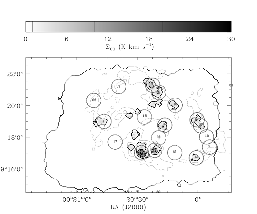
Figure 5.— The integrated intensity map resulting from the BIMA D-array survey and the locations of the UASO 12m pointings. The ARO 12m pointings cover most of the CO emission from IC 10. Light contours indicate $\Sigma_{HI}$ = 10, 20, and 30 M_⊙ pc^-2 (Wilcots & Miller, 1998). Several ARO 12m pointings are outside this figure, and appear along the edges. The extent of the survey is indicated by the solid black lines.

3.3. Other Data Used in This Paper

3.3.1 OVRO High Resolution CO Maps

We use the high resolution OVRO observations of IC 10 presented by Walter (2003) to study spatially resolved GMCs and as a third point of comparison for CO fluxes and line widths. These data have an angular resolution (FWHM) of $3.4\arcsec$ ($13.5$ pc) or $4.9\arcsec$ ($19.5$ pc), depending on the location in the galaxy, and a velocity resolution of $\approx 0.65$ km s^-1. The high resolution and good signal-to-noise ratio in these data allow us to measure the properties of individual GMCs. The OVRO primary beam is $\sim 50\arcsec$ at 115 GHz, so these data are not sensitive at all to spatial scales more extended than $\sim 25\arcsec$.

3.3.2 H$\alpha$ Imaging

We use an H$\alpha$ image of IC 10 from Gil de Paz et al. (2003) to measure the star formation per unit area ($\Sigma_{SFR}$) across IC 10. We correct the H$\alpha$ intensity for the effects of extinction and then convert to $\Sigma_{SFR}$ using the calibration by Kennicutt et al. (1994),

$$SFR~{}\left[\frac{\mbox{M}_{\odot}}{\mbox{yr}}\right]=\frac{L(H\alpha)}{1.26\times 10^{41}~{}\mbox{erg s}^{-1}}~{}\mbox{,}$$ (3)

which assumes a Salpeter IMF (from 0.1 to 100 M_⊙).

Because IC 10 lies near the Galactic plane, foreground extinction is important. We assume a reddening towards IC 10 of $E(B-V)=0.77$ (Massey & Armandroff, 1995; Hunter, 2001), which corresponds to an $R$-band extinction of $\approx 2$ magnitudes for a Galactic extinction law (Cardelli et al., 1989). This extinction is consistent with the Galactic dust column near IC 10 in each direction in the dust map of Schlegel et al. (1998). Our value is lower than the extinction adopted by Gil de Paz et al. (2003), who derive their extinction from the Schlegel et al. (1998) pointing directly towards IC 10. That pointing may be confused by FIR emission from the galaxy itself.

We adjust the H$\alpha$ fluxes from IC 10 to account for 1.1 magnitudes of internal extinction but this is a large source of uncertainty. The reddening extinction towards unembedded stars is due overwhelmingly to Galactic dust (Hunter, 2001). However, Yang & Skillman (1993) and Borissova et al. (2000) compare radio continuum and Br$\gamma$ fluxes to H$\alpha$ and find additional reddenings of $E(B-V)\sim 1$ (total $E(B-V)\sim 1.5$ – $2$) towards embedded HII regions, implying extinctions as high as $A_{R}\sim 2.6$ towards these sources. Most of the H$\alpha$ emission from IC 10 comes from regions that are at least somewhat embedded (see Figure 2): 80% comes from lines of sight with H I columns above 10 M_⊙ pc^-2 ($1.25\times 10^{21}$ cm^-2) and the mean H I column associated with a bit of H$\alpha$ emission ( $\sum I(H\alpha)N(\mbox{\rm{H~{}I}})/\sum I(H\alpha)$ ) is $15$ M_⊙ pc^-2. In the Milky Way, this column of gas (assuming it all lies between the observer and the H$\alpha$) implies a reddening of $E(B-V)\sim 0.4$ (Bohlin et al., 1978) and a corresponding $R$-band extinction of $\sim 1.0$ magnitudes. Of course, the H I column is unlikely to all lie in front of the H$\alpha$ emission, but there is a contribution from dust associated with molecular gas, as well. We use the H$\alpha$ map to test the applicability of a “Schmidt Law” to IC 10 and this value is similar to the 1.1 magnitudes of internal extinction assumed by Kennicutt (1998), so we adopt that value (1.1) for consistency but note it to be uncertain by $\sim 1$ magnitude.

3.3.3 VLA High Resolution HI Map

We use the high resolution VLA H I map of Wilcots & Miller (1998), reduced using natural weighting, which has a resolution of $11\arcsec$ (44 pc). The VLA map contains mostly data from intermediate arrays (B and C, minimum baseline $\sim 35$ m, with just 10 minutes of D array data) and is therefore not sensitive to spatial scales $\gtrsim 15$′(although power on scales as small as $\sim 7.5$′may be attenuated by $\sim 40\%$). In this work, we are interested in the H I over the central disk (where the CO is). In this region the structure of the H I varies on $\sim 1$′ scales (the holes and filaments in Figure 1) and we do not expect significant loss of power on these scales. However, the H I surrounding IC 10 is very extended and spatial filtering is important to large scale studies. For example, Wilcots & Miller (1998) find only 60% of the flux recovered by Shostak & Skillman (1989) using the WSRT. In turn, Shostak & Skillman (1989) recover only half of the value found by single dish telescopes. The extended emission being resolved out by the interferometers has low column density ($\sim 1\times 10^{20}$ cm^-2 Wilcots & Miller, 1998), a factor of $\sim 10$ lower than the typical columns associated with CO detection (see Shostak & Skillman, 1989, for a map of extended emission missed by the WSRT). The large flux discrepancies come from the large spatial extent of the H I and should only represent a $\sim 10\%$ correction on the compact, high column structures associated with the CO.

3.3.4 $K$-band Photometry

IC 10 is part of the 2MASS Large Galaxy Atlas (Jarrett et al., 2003). We use the $K$-band image to trace the stellar population in IC 10. Because IC 10 is at a low Galactic latitude ($b=-3.3^{\circ}$) foreground stars represent a serious source of contamination. In order to remove these foreground stars, we mask out the brightest pixels in the 2MASS image. Our threshold for identifying “bright pixels” corresponds to a stellar surface density of $1800$ M_⊙ pc^-2. We removed all pixels above this value from the image, as well as all data adjacent to these pixels with a surface density of $\approx 600$ M_⊙ pc^-2 (to ensure that we clipped the tail of the point spread function for the stars we remove). The highest stellar surface density we find for the disk of IC 10 is $\lesssim 500$ M_⊙, so the galaxy should be unaffected by the masking. After removing bright pixels, we apply a $15^{\prime\prime}$ median filter to the whole image, using the median values to replace the data we removed. Finally, we adopt a $K$-band mass to light ratio of $0.5$ M_⊙ / L_⊙,K, consistent with the results found by Simon et al. (2005) in their study of rotation curves of dwarf galaxies. The scatter they find in their mass-to-light ratios is $\approx 50\%$ (ranging from $0.3$ to $0.7$ M_⊙ / L_⊙,K) so the stellar surface density is uncertain by the same amount. The resulting $K$-band surface density map has a resolution comparable to the BIMA survey (because of the filtering) and is largely uncontaminated by bright foreground stars. Figure 1 shows this map as contours plotted over the extended H I distribution.

3.4. Overview of GMC Property Measurements

This section summarizes the algorithm described in detail by Rosolowsky & Leroy (2005), which we use to measure resolved GMC properties and correct these measurements for biases introduced by our limited resolution and sensitivity. We apply this algorithm to the BIMA survey and to the high resolution OVRO data sets from Walter (2003) to produce the cloud property measurements in Tables 4 and 5.

First, we construct a mask containing all high significance signal in the data cubes. For the BIMA survey we use the mask generated as described in §3.1.2 and simply assign emission to the nearest local maximum (see the cloud assignments in Figure 4). For the OVRO data, we include all regions with two adjacent velocity channels both containing emission above $4\sigma$ intensity. We expand the mask to include all emission with two adjacent velocity channels above $2\sigma$ that is contiguous with the $4\sigma$ peaks. We then identify significant, independent local maxima within each cloud. Here “significant” means that the maxima are at a significantly higher intensity ($2\sigma$ greater) than either the edge of the cloud or the highest isosurface shared with other local maxima. An “independent” maximum is separated from all other maxima by at least a velocity channel or a full beam width.

From the emission uniquely associated with each maximum (i.e. within the lowest isosurface containing only that maximum), we measure the size, line width, and luminosity for that cloud. We make the measurements using intensity-weighted moment methods (i.e. we measure spatial and velocity dispersions). From the measured dispersions, we calculate the radius of the cloud using the definition of Solomon et al. (1987). The line width is the full-width at half-maximum of the integrated spectrum of the cloud. The luminosity is the integrated emission from the cloud. We correct these measurements for biases due to the finite sensitivity and resolution of the astronomical data. We correct for the finite sensitivity by extrapolating the measured properties to those we would expect for a data set with perfect sensitivity (by fitting each property as a function of boundary isosurface value and extrapolating to a boundary of $0$ K). We correct for the effects of beam convolution on the measured size of the GMCs by deconvolving the beam size from the measured size in quadrature (separately for the major and minor axes). Since the detailed description of the algorithm and its characterization is beyond the scope of this paper, we refer the reader to Rosolowsky & Leroy (2005).

Table 4 Cloud Properties from the BIMA Survey

Cloud #	$\alpha$	$\delta$	$v_{ctr}$	$V_{FWHM}$	Luminosity	$M_{Lum}$
	(J2000)	(J2000)	(km s-1)	(km s-1)	($10^{3}$ K km s-1 pc2)	($10^{3}$ M⊙)
(1)	(2)	(3)	(4)	(5)	(6)	(7)
B1	0h 19m 58.6s	59∘ 18′ 40.6$"$	-367.4	7.7	30.	131.
B2	0h 20m 0.8s	59∘ 19′ 4.9$"$	-366.3	12.4	38.	164.
B3	0h 20m 1.3s	59∘ 16′ 42.3$"$	-364.0	16.1	49.	213.
B4	0h 20m 11.9s	59∘ 20′ 2.2$"$	-343.6	13.6	51.	221.
B5	0h 20m 17.2s	59∘ 18′ 43.3$"$	-335.9	17.4	50.	218.
B6	0h 20m 19.6s	59∘ 20′ 48.1$"$	-337.8	10.5	75.	326.
B7	0h 20m 21.2s	59∘ 20′ 8.1$"$	-330.6	11.4	41.	180.
B8	0h 20m 21.6s	59∘ 17′ 8.8$"$	-339.7	10.5	102.	443.
B9	0h 20m 22.9s	59∘ 21′ 18.3$"$	-329.6	7.5	122.	533.
B10	0h 20m 27.6s	59∘ 17′ 26.2$"$	-329.6	15.3	57.	246.
B11	0h 20m 27.7s	59∘ 16′ 59.4$"$	-330.9	14.9	238.	1036.
B12	0h 20m 29.8s	59∘ 19′ 34.0$"$	-326.4	4.8	12.	52.
B13	0h 20m 31.3s	59∘ 18′ 9.9$"$	-324.5	12.0	25.	110.
B14	0h 20m 32.6s	59∘ 17′ 21.6$"$	-311.1	15.0	11.	48.
B15	0h 20m 34.4s	59∘ 19′ 24.0$"$	-317.7	21.4	17.	76.
B16	0h 20m 48.1s	59∘ 18′ 58.1$"$	-330.5	13.9	61.	266.

Table 5 GMC Properties in IC 10

Cloud	$\alpha$	$\delta$	$v_{ctr}$	Radius	$V_{FWHM}$	Luminosity	$\log_{10}~{}M_{Lum}$	$\log_{10}~{}M_{vir}$	$M_{Vir}$/$M_{Lum}$
	(J2000)	(J2000)	(km s-1)	(pc)	(km s-1)	($10^{3}$ K km s-1 pc2)	(M⊙)	(M⊙)
(1)	(2)	(3)	(4)	(5)	(6)	(7)	(8)	(9)	(10)
B1	0h 19m 58.6s	59∘ 18′ 40.3$"$	-366.6	11.8 $\pm$ 6.1	4.0 $\pm$ 1.0	13.4 $\pm$ 2.8	4.8 $\pm$ 0.1	4.6 $\pm$ 0.2	0.6 $\pm$ 0.5
B2	0h 20m 0.9s	59∘ 19′ 2.2$"$	-367.4	22.8 $\pm$ 9.6	5.7 $\pm$ 2.0	9.6 $\pm$ 7.0	4.6 $\pm$ 0.2	5.1 $\pm$ 0.3	3.3 $\pm$ 3.8
B4	0h 20m 12.0s	59∘ 20′ 2.5$"$	-342.7	29.4 $\pm$ 7.2	5.6 $\pm$ 1.0	20.2 $\pm$ 2.7	4.9 $\pm$ 0.1	5.2 $\pm$ 0.2	2.0 $\pm$ 1.1
B5	0h 20m 17.3s	59∘ 18′ 42.0$"$	-334.0	26.2 $\pm$ 5.5	6.2 $\pm$ 1.3	25.3 $\pm$ 4.7	5.0 $\pm$ 0.1	5.3 $\pm$ 0.2	1.7 $\pm$ 1.0
B6	0h 20m 19.6s	59∘ 20′ 48.0$"$	-338.2	17.7 $\pm$ 3.9	6.0 $\pm$ 1.2	27.5 $\pm$ 5.3	5.1 $\pm$ 0.1	5.1 $\pm$ 0.2	1.0 $\pm$ 0.5
B8	0h 20m 21.7s	59∘ 17′ 9.6$"$	-339.5	24.1 $\pm$ 2.6	6.1 $\pm$ 0.6	69.5 $\pm$ 3.2	5.5 $\pm$ 0.0	5.2 $\pm$ 0.1	0.6 $\pm$ 0.1
B7	0h 20m 22.1s	59∘ 20′ 4.9$"$	-329.3	18.3 $\pm$ 6.3	4.0 $\pm$ 1.1	18.0 $\pm$ 5.4	4.9 $\pm$ 0.1	4.7 $\pm$ 0.2	0.7 $\pm$ 0.5
B9a	0h 20m 22.3s	59∘ 21′ 5.6$"$	-330.5	15.9 $\pm$ 4.6	3.0 $\pm$ 0.8	14.1 $\pm$ 3.2	4.8 $\pm$ 0.1	4.4 $\pm$ 0.2	0.4 $\pm$ 0.3
B9b	0h 20m 22.5s	59∘ 21′ 21.4$"$	-328.7	24.5 $\pm$ 6.3	4.3 $\pm$ 1.1	18.7 $\pm$ 5.3	4.9 $\pm$ 0.1	4.9 $\pm$ 0.2	1.1 $\pm$ 0.7
B9c	0h 20m 23.7s	59∘ 21′ 17.9$"$	-333.8	27.2 $\pm$ 7.7	5.5 $\pm$ 2.5	22.4 $\pm$ 5.8	5.0 $\pm$ 0.1	5.2 $\pm$ 0.3	1.6 $\pm$ 1.5
B11a	0h 20m 27.2s	59∘ 16′ 53.8$"$	-334.0	22.1 $\pm$ 7.3	10.4 $\pm$ 2.5	76.4 $\pm$ 24.1	5.5 $\pm$ 0.1	5.7 $\pm$ 0.2	1.4 $\pm$ 1.0
B11b	0h 20m 27.3s	59∘ 17′ 5.5$"$	-331.1	14.9 $\pm$ 3.0	7.4 $\pm$ 1.1	52.5 $\pm$ 8.5	5.4 $\pm$ 0.1	5.2 $\pm$ 0.1	0.7 $\pm$ 0.3
B11c	0h 20m 28.1s	59∘ 16′ 57.0$"$	-325.1	17.8 $\pm$ 4.5	11.2 $\pm$ 2.2	64.3 $\pm$ 12.0	5.4 $\pm$ 0.1	5.6 $\pm$ 0.2	1.5 $\pm$ 0.8
B11d	0h 20m 29.0s	59∘ 17′ 4.6$"$	-327.4	18.4 $\pm$ 3.9	7.9 $\pm$ 1.5	25.6 $\pm$ 4.8	5.0 $\pm$ 0.1	5.3 $\pm$ 0.2	1.9 $\pm$ 1.0

4. Results

4.1. Comparison of the Three CO Datasets

How do the emission properties from the BIMA survey, the ARO 12m data, and the OVRO observations compare? We convolved the BIMA survey, OVRO data, and the H I data (first clipped at 3$\sigma$) to the resolution of the ARO 12m data. Figure 6 shows these data for each ARO 12m pointing with detected emission (the H I spectra are arbitrarily normalized). Based on these spectra and Figure 5 we draw the following conclusions:

1. The agreement between the central velocities among all three datasets is excellent. Further, the velocities are consistent with the H I emission (dashed line in Figure 6). Towards the brightest lines, the width of CO emission detected by the ARO 12m is comparable to, but always a bit smaller than, that of the H I emission.

2. Both interferometers miss emission, and OVRO misses more than BIMA. This is probably a result of interferometers filtering out extended emission and not due to low signal-to-noise or to calibration errors. Both the BIMA survey and the OVRO data are more sensitive than the ARO 12m (both data sets have RMS noise $<10$ mK over an ARO 12m beam at $6$ km s^-1 velocity resolution, compared to a typical noise of $15$ mK for the ARO 12m spectra). Further, the OVRO data are missing more flux than the BIMA survey, despite having a better signal-to-noise. Finally, the difference is not only a gain offset, as one would expect from a calibration discrepancy. Rather, the line widths of the interferometer data (particularly the OVRO data) are smaller than those found by the single dish, implying that an extended component with a larger velocity width contributes to the single dish data but not the interferometer data.

How much emission is resolved out by the interferometers? On average, BIMA recovers $50\%$ of the integrated intensity found by the ARO 12m, and OVRO recovers $30\%$. BIMA finds a line width that is on average $90\%$ of that recovered by the ARO 12m, while OVRO line widths are, on average, $60\%$ that of the ARO 12m for the same pointing. We simulated BIMA D array observations of several gaussian sources at the declination of IC 10. The observations recover 95$\%$ of the flux for a 20″ (FWHM) source, 60% for a 30″ source, 30% for a 40″ source, and 14% for a 40″ source. If the CO structures in IC 10 are $\sim 35$″ (160 pc) we might expect to lose half of the flux. The actual scales may be slighly more compact since there are inefficiencies associated with signal identification and non-ideal observing conditions that will affect diffuse emission or long baselines.

3. We detect CO emission with the ARO 12m only at pointings which also show emission in the BIMA survey (see point 4). Therefore the diffuse emission appears to be associated with the larger GMCs. Further, the ARO 12m pointings cover almost all of the CO emission found in the BIMA survey. Only $\sim 1\times 10^{5}$ K km s^-1 pc² (BIMA clouds 7, 12, 13, 14, and 15) of the emission from the BIMA survey (about 10% of the total) lies in clouds not targeted by the ARO 12m pointings.

4. Two pointings deserve specific commentary: numbers 7 and 14. Pointing 7 is detected by the ARO 12m and Figure 6 shows that it is also detected in the BIMA survey. However, the emission is not strong enough to be included in our mask. Pointing 14 is detected in the BIMA survey, but the ARO 12m emission appears to be contaminated by emission in the off position.

Our comparison of the three data sets suggests that $\sim 50\%$ of the CO emission from IC 10 comes from a high velocity width, spatially extended component that is resolved out by both OVRO and BIMA. OVRO further resolves out another 20% of the CO emission seen by the ARO 12m. Similar results have been found in the Milky Way, M 31 and M 33 (Polk et al., 1988; Blitz, 1985; Rosolowsky et al., 2003). In those galaxies, too, diffuse gas, or an extended grouping of small molecular clouds indistinguishable from diffuse gas, may contribute a large portion of the CO emission along a line of sight.

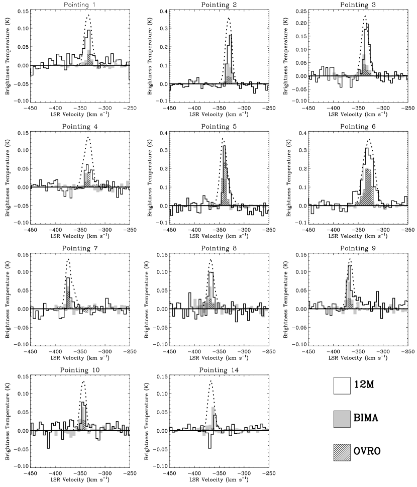
Figure 6.— ARO 12m, BIMA, and OVRO spectra compared for common pointings which show emission. The BIMA and OVRO data have been convolved to the resolution of the ARO 12m. The H I spectrum, normalized to 80% of the $y$-axis range, is overplotted as a dashed line to indicated the velocity width of the H I.

4.2. The Total Content of Molecular Gas and GMC Properties

Figure 4 and Table 4 present the results of the BIMA survey. The total luminosity from all 10 CO detections with the ARO 12m of $1.6\pm 0.3\times 10^{6}$ K km s^-1 pc² and this is our formal lower limit to the total CO luminosity of IC 10. If we stack all of the ARO pointings and integrate, the luminosity rises to $2.0\times 10^{6}$ K km s^-1 pc² with the increase of 25% due emission not detected in individual pointings (a signature of a low-intensity diffuse component, perhaps similar to that found by Israel, 1997). The ARO 12m pointings overlap $\sim 90\%$ of the emission found in the BIMA survey, so we estimate that the total CO luminosity of IC 10 is $\sim 2\times 10^{6}\times\frac{1}{0.9}=2.2\times 10^{6}$ K km s^-1 pc². This number is quite uncertain because our masking algorithm is chosen to avoid false positives (rather than for completeness). We estimate an upper limit by noting that the inclusion of 11 pointings without individual CO detections raises the integrated luminosity by $\sim 4\times 10^{5}$ K km s^-1 pc². The total area in IC 10 with an H I surface density $>10$ M_⊙ pc² (and therefore likely to harbor molecular gas) corresponds to $\sim 16$ times the area of the 12m beam. Of this area about $6$ times the area of the 12m beam is already covered by our ARO observations. Four of our nondetection pointings are extremely unlikely sites for molecular gas emission. Therefore, we might expect another $\frac{10}{7}\times(4\times 10^{5})\sim 6\times 10^{6}$ K km s^-1 pc² in diffuse emission. We therefore suggest $2.8\times 10^{6}$ K km s^-1 pc² as an upper limit to the CO luminosity. The BIMA survey recovers about half of our best guess at the luminosity — the 16 GMCs listed in Table 4 have a total luminosity of $1.0\times 10^{6}~{}$ K km s^-1 pc² (which includes a $\sim 30\%$ sensitivity correction as described in §3.4).

We used the algorithm of Rosolowsky & Leroy (2005) summarized in §3.4 to identify clouds and then measure their properties using the OVRO dataset (Walter, 2003). Table 5 gives our measurements of the properties of $14$ GMCs. Column (1) gives the cloud name (which also indicates the BIMA survey cloud to which the OVRO cloud most nearly corresponds); columns (2) and (3) give the intensity-weighted average position of the cloud; column (4) gives the intensity-weighted average velocity of emission from the cloud; column (5) gives the equivalent spherical radius of the cloud (Solomon et al., 1987) in parsecs, after correction for the effects of beam convolution; column (6) gives the FWHM line width of the cloud; column (7) gives the cloud luminosity in K km s^-1 pc²; column (8) gives the mass derived from this luminosity assuming a Galactic CO-to-H₂ conversion factor; column (9) gives the dynamical mass of the cloud, calculated assuming virial equilibrium and a $\rho\propto r^{-1}$ density profile, so that $M_{vir}=189~{}R~{}V_{FWHM}^{2}$, with $R$ and $V_{FWHM}$ as defined above; column (10) gives the ratio of virial to luminous mass for the cloud. The virial masses are comparable to the luminous masses, suggesting that the CO-to-H₂ conversion factor does not vary significantly from the Galactic value. Figure 7 shows a map each of cloud. Ellipses indicate the size of each cloud before any corrections for resolution or sensitivity effects are applied, so that the sizes shown is directly comparable to the structures in the data. In Table 5 and in the analysis below, however, we use the corrected values.

We include a brief word of warning regarding cloud names. For clarity we refer to clouds measured in the OVRO data using the same system we used for the BIMA survey, using “a,b,c” when a BIMA cloud is resolved into several GMCs by OVRO. However, we have not tried to systematically identify a single set of clouds using both data sets, and the association implied by a shared name should not be weighted too heavily. For example, though no cloud B10 exists in the OVRO data, emission from that object certainly corresponds to some of the emission found in clouds B11a,b,c, and d.

4.3. Comparison to GMC Properties From the Literature

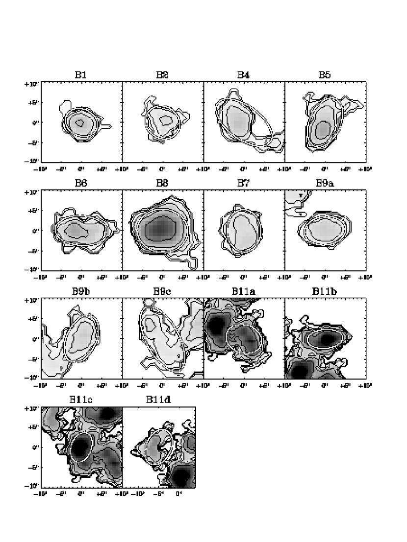
Figure 7.— Intensity maps of GMCs in IC 10. The figure shows all CO emission near the center of the GMC. The circles indicate the measured sizes of the GMC sensitivity or resolution corrections. At the distance of IC 10 ($950$ kpc), $1\arcsec$ corresponds to 4.6 pc, so the $40\arcsec$ boxes shown have spatial sizes of $92$ pc.

There are several observations of IC 10 GMCs in the literature: do the properties we measure agree with these studies? Table 6 shows a comparison of the properties of three GMCs in the bright CO complex in the southeast part of the galaxy (cloud 15 in Figure 4, ARO 12m pointing 6 in Figure 5). Table 6 shows the properties measured by two previous studies (Wilson, 1995; Ohta et al., 1992) and this work. All three works decompose the emission in essentially the same manner, though some of the variations in Table 6 may arise from decisions about which emission to assign to which GMC. To properly compare these observations we have adjusted the sizes measured by the two previous studies to match our definition of the radius, our adopted distance, and our adopted Galactic CO-to-H₂ conversion factor — both Ohta et al. (1992) and Wilson (1995) quote full width half maximum sizes and they adopt distances of 1.3 and 0.82 Mpc, respectively. Ohta et al. (1992) labels the GMCs in question ’NC1,’ ’NC2,’ and ’SC’ (1, 2, and 3 in Table 6); Wilson (1995) calls them ’MC1,’ ’MC2,’ and ’MC3;’ they are ’B11b,’ ’B11c,’ and ’B11a,’ respectively, in our Table 5. The sizes agree well for two of the three clouds, and we measure a notably lower size for GMC 1; there is a significant ($\sim 50\%$) scatter in the line widths. The fluxes measured by Wilson (1995) are systematically lower than what we measure — integrated over the complex, Wilson (1995) measures half of our flux. The discrepancy in fluxes and our 15% larger adopted distance explain why Wilson (1995) derives a higher CO-to-H₂ conversion factor for the GMCs than we do. The combination of a larger adopted distance and the systematically higher fluxes found by Ohta et al. (1992) explain the similarity in the derived CO-to-H₂ conversion factors.

Which measurements are closer to the true fluxes? The complex in question corresponds to pointing 6 with the ARO 12m (see Figures 5 and 6 and Table 3) and cloud BIMA 11 in Table 4. BIMA and OVRO find similar fluxes for the region (both corresponding to $\approx 10^{6}$ M_⊙ for our adopted X_CO) and the ARO 12m recovers about 2.5 times this luminosity. Wilson (1995) finds fluxes lower than those found by BIMA, the newer OVRO dataset, or the ARO 12m. The NMA dataset appears consistent with the BIMA and OVRO results (also finding $\approx 10^{6}$ M_⊙ for our X_CO). Therefore the Wilson (1995) fluxes represent an outlier from the other interferometric data. All four interferometric data sets resolve out a large fraction of the flux (as measured by the ARO 12m).

Table 6 IC 10 SE GMC Property Comparison

GMC	Property	Ohta et al. (1992)	Wilson (1995)	This Paper
1	Radius (pc)	$23$	$32$	$15$
1	$V_{FWHM}$ (km s-1)	$7.3$	$10.9$	$7.4$
1	Luminous Mass ($10^{3}$ M⊙)	$290$	$190$	$250$
2	Radius (pc)	$19$	$23$	$18$
2	$V_{FWHM}$ (km s-1)	$7.3$	$8.9$	$11.2$
2	Luminous Mass ($10^{3}$ M⊙)	$230$	$120$	$250$
3	Radius (pc)	$24$	$24$	$22$
3	$V_{FWHM}$ (km s-1)	$<8.2$	$12.8$	$10.4$
3	Luminous Mass ($10^{3}$ M⊙)	$490$	$130$	$320$

5. Discussion

5.1. Molecular Gas Fraction and Depletion Time

Using a Galactic CO-to-H₂ conversion factor, $2\times 10^{20}$ cm^-2 (K km s^-1)^-1(appropriate for the GMCs but perhaps not for diffuse gas, see §5.2), the luminosity we estimate for IC 10 translates to a molecular gas mass of $9\times 10^{6}$ M_⊙. This mass is small compared to the other components of IC 10 — the stellar, H I  and dynamical masses are $\sim 4,~{}2,$ and $15\times 10^{8}$ M_⊙ respectively — and this implies that only $4\%$ of the gas is molecular. For a star formation rate of $\sim 0.2$ M_⊙ yr^-1, the depletion time for the molecular gas associated with CO in IC 10 is $\sim 4\times 10^{7}$ years, compared to the median depletion time of $2\times 10^{9}$ years found in nearby dwarf galaxies (Leroy et al., 2005). The molecular gas mass is only about $\sim 2\%$ of the stellar mass. This value tends to be larger, $\sim 15\%$, in LMC-type dwarf galaxies (Young & Scoville, 1991; Leroy et al., 2005). In fact, the amount of molecular gas per stellar luminosity tends to be fairly constant among all star forming galaxies, large and small (in the $K$-band this ratio is $\sim 0.07$ M_⊙ / L_K,⊙ Leroy et al., 2005). Although IC 10 is CO-deficient compared to larger galaxies, it is CO-rich when compared to the SMC or NGC 1569. Mizuno et al. (2001) find that the CO luminosity of the SMC is $\approx 8\times 10^{4}$ K km s^-1 pc², more than an order of magnitude fainter than the CO luminosity of IC 10, while NGC 1569, which has a CO luminosity of $\sim 10^{5}$ K km s^-1 pc² (Greve et al., 1996; Taylor et al., 1999). This yields an even shorter molecular gas depletion time for these two systems than what we observe in IC 10.

5.2. The CO-to-H₂ Conversion Factor in IC 10

With lower abundances of carbon and oxygen, harder radiation fields, and less dust to shield each parcel of gas, dwarf galaxies may be expected to display a different relationship between CO emission and molecular hydrogen content. Calibrating the CO-to-H₂ conversion factor, $X_{CO}$, has often been a goal of CO studies of dwarf galaxies (e.g. Wilson, 1995). The key to measuring $X_{CO}$ in other galaxies is to find an independent method of measuring the amount of molecular gas present. We attempt an independent estimate of the mass by measuring the size and line width of a molecular cloud from its CO emission and then calculating the dynamical mass under the assumption of virial equilibrium.

In our analysis of the high resolution CO data, we find that the IC 10 clouds are indistinguishable from GMCs analyzed in the same way in M 31 and M 33 and that they are very similar to Milky Way clouds. If the IC 10 clouds are virialized, then the mean CO-to-H₂ conversion factor in the CO peaks is $2.6\times 10^{20}$ cm^-2 (K km s^-1)^-1 (if the clouds are only marginally bound then X_CO will be half of this value). Virial mass studies in the Milky Way yield a CO-to-H₂ conversion factor $\mbox{\rm X${}_{\rm CO}$}\approx 3\times 10^{20}$ cm^-2 (K km s^-1)^-1(Solomon et al., 1987), similar to the one we measure in IC 10 within the uncertainties; interferometric studies of M 31 and M 33 yield approximately the same result Rosolowsky et al. (2003); Rosolowsky & Leroy (2005). Because, in the Milky Way, the X_CO value derived from gamma-ray observations is thought by many to be more reliable (it is independent of the dynamical state of the GMCs), we adopt the Galactic value of $X_{CO}$ obtained by those studies, $2\times 10^{20}$ cm^-2 (K km s^-1)^-1 (Strong & Mattox, 1996; Dame et al., 2001) in the remainder of this study.

In §4.1 we found that OVRO may resolve out $70\%$ of the emission. The measurements of the GMC properties are probably robust, since the GMCs are compact relative to the $\sim 100$ pc scales we expect OVRO to resolve out and the OVRO data have good sensitivity. However, the GMC properties measured from the OVRO data do not constrain the CO-to-H₂ conversion factor in the extended emission. One possibility is that the CO resolved out by OVRO and BIMA comes from a spatially extended collection of small GMCs. Below we find evidence for a GMC mass spectrum with a power law index of $-2.0$, which implies that there may be as much mass in GMCs below our completeness limit as above it. If these low mass GMCs make up the extended structure that is resolved out by BIMA and OVRO, then we expect that the CO-to-H₂ conversion factor from the OVRO clouds will apply, at least approximately, to all of the CO emission.

Based on observations of the 158 $\mu$m [CII] emission line, Madden et al. (1997) suggested a CO-to-H₂ conversion factor much higher than the Galactic value. They mapped IC 10 at $\sim 1^{\prime}$ resolution and found that it is luminous in the [CII] line compared to the CO luminosity. In the northern and western regions, they found that the minimum amount of hydrogen needed to produce the observed [CII] emission implies a substantial mass of gas that was not inferred from the H I or CO emission. They suggested that in parts of IC 10 molecular hydrogen may exist under conditions of low extinction, $A_{V}\sim 1$ – $2$, so that CO is dissociated but self-shielded H₂ is abundant. They argue that in these regions the H₂ column may exceed the H I column by a factor of 5. Although we adopt a Galactic X_CO, we can not rule out the evidence of Madden et al. (1997) for a large reservoir of non-CO-emitting molecular gas outside the central GMCs. We do not account for such gas in our discussion of star formation efficiencies because such gas must be warm, diffuse, poorly shielded, and, as such, does not seem to be a likely locale for star formation (the excitation temperature of the 158 $\mu$m [CII] line is 92 K and the CO-free molecular gas posited by Madden et al. (1997) exists at extinctions of $A_{V}\sim 1$ – $2$ magnitudes). Further, if such gas exists in other galaxies it will be similarly unaccounted for by the CO luminosity and should thus be left out for a self-consistent comparison.

There may be evidence for a reservoir of warm, CO-free H₂ beyond the GMCs, however observations do not suggest the presence of a hidden reservoir of cold gas. In a study of the dust continuum in the southeast part of IC 10, Bolatto et al. (2000) considered and rejected the possibility of a large reservoir of cold molecular gas in that region. Although they find an excess of long wavelength infrared emission, they cite the lack of CO self absorption and the normal CO ($2\rightarrow 1$) to CO ($1\rightarrow 0$) ratios as evidence that the long wavelength emission is not indicative of a massive reservoir of cold molecular gas. Thronson et al. (1990) also finds the amount of 155 $\mu$m dust emission in IC 10 to be consistent with the H I emission from the galaxy. A large population of hidden molecular gas is not necessary to explain their observations, though IC 10 does show a mild excess at 155 $\mu$m.

For the rest of this paper, we adopt a CO-to-H₂ conversion factor of $2\times 10^{20}$ cm^-2 (K km s^-1)^-1 for all of the CO emission. We are confident in the applicability of this value of X_CO to the GMCs but less certain whether it is appropriate for diffuse CO emission. We neglect the possibility of warm H₂ untraced by CO because we have no observational handle on such gas and it seems unlikely to form stars, but we emphasize that any such excess of molecular gas must exist outside the most massive GMCs or we would see evidence for it in the virial masses we measure from the OVRO data. We note the following conversions for our adopted X_CO: an integrated intensity of 1 K km s^-1 corresponds to a molecular gas surface density of 4.4 M_⊙ pc^-2, including helium, and therefore a luminosity of 1 K km s^-1 pc² translates into a molecular mass of 4.4 $M_{\odot}$.

5.3. Mass-Size-Line Width Relations in IC 10

In the Milky Way, M 33, and M 31 molecular gas is concentrated in GMCs which exhibit scaling laws relating their properties (Solomon et al., 1987; Rosolowsky et al., 2003; Rosolowsky, 2005). These relationships, often referred to as “Larson’s Laws,” (Larson, 1981) relate the size of a GMC to its line width, the CO luminosity to the dynamical mass, and the luminosity to the line width. In this section we compare clouds in IC 10 to clouds from the Milky Way, M 33, and M 31. M 31 and M 33 are at distances comparable to that of IC 10, $\lesssim 1$ Mpc, and the interferometric data used for the comparison have similar spatial resolutions ($\approx 20$ pc). We measure their properties using the same algorithm used to analyze the IC 10 clouds (a reanalysis of the data presented in Rosolowsky et al., 2003; Rosolowsky, 2005). Thus the M 31 and M 33 data should represent an excellent “control” sample, and any differences between GMC properties in these systems and IC 10 should be a result mainly of environmental factors, not observational or analytical biases. The Milky Way data have not been analyzed in the same manner as the other data sets — they just consist of the GMC properties measured by Solomon et al. (1987) — so systematic differences may bias the comparison. However, we have attempted to correct for sensitivity and resolution biases in our data and the Solomon et al. (1987) data have good sensitivity and spatial resolution (being Galactic data) so we anticipate the magnitude of these biases to be small.

Figure 8 shows that clouds in IC 10 lie on or near the scaling laws for GMCs in the Milky Way, M 31, and M 33. This conclusion is reinforced by Figure 9, which shows three physical parameters — the surface density, the virial to luminous mass ratio, and the scatter about the size-velocity dispersion relation ($\sigma_{v}\propto R^{0.5}$) — for clouds in IC 10, the Milky Way, M 31, and M 33. Table 7 show the results of two sided KS-tests comparing these physical parameters between IC 10 and the Milky Way (column 2) and M 31+M 33 (column 3). The distribution of physical parameters for IC 10 GMCs agrees very well with the distribution found for the M 31 and M 33 GMCs ($<2\sigma$ difference for each parameter). Since the M31/M33 GMC properties are also derived from interferometric data and are the result of the same analysis used to produce the IC 10 GMC properties, we attach particular weight to this comparison. The KS test detects $\sim 3\sigma$ differences between in IC 10 the Milky Way in the both surface density of clouds and their scatter about the size-velocity dispersion relation. Figure 9 shows that these differences are relatively small however and since the same differences exist between the Milky Way data and the M 31/M 33 data they may represent a systematic difference stemming from either observational biases or differences in the measurement algorithm. The CO-emitting clouds resolved by OVRO in IC 10 are very similar to GMCs in the Milky Way. They are indistinguishable from GMCs in M 31 and M 33 observed and analyzed in the same manner as the IC 10 clouds.

Table 7 KS Test Comparisons of IC 10 GMCs

Property	vs. Milky Way	vs. M 31+M 33
Surface Density	$0.02$	$0.65$
Size 0.5 / Velocity Dispersion	$1\times 10^{-3}$	$0.41$
Virial Parameter	$0.25$	$0.67$

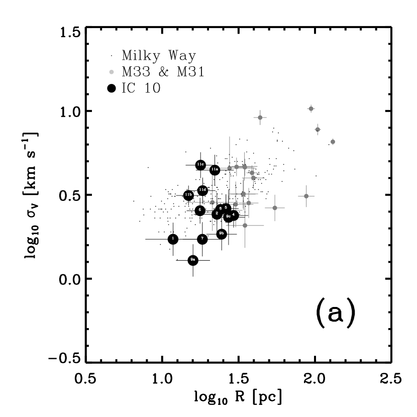
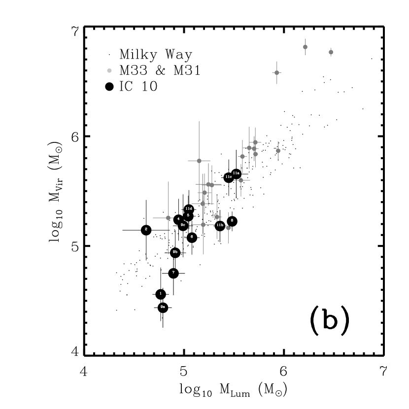
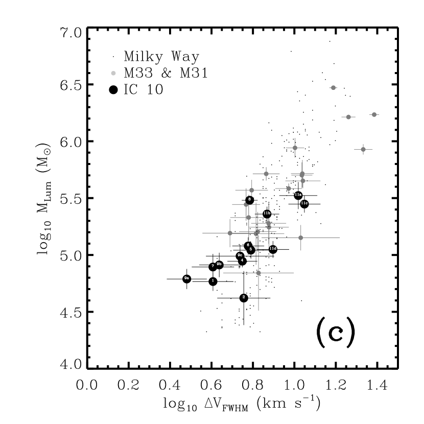
Figure 8.— Larson’s laws for clouds in IC 10 (black circles), compared to the Milky Way (black dots) and the Local Group spirals M 31 and M 33 (gray circles). (a) The size-velocity dispersion relation. (b) The virial mass-luminosity relationship. (c) The luminosity-line width relationship. All four galaxies display very similar behavior, obeying the same scaling of their global GMC properties.

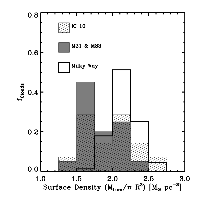
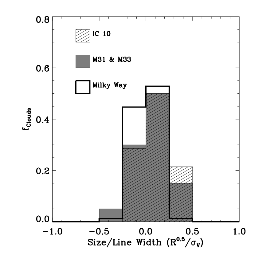
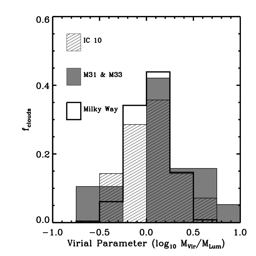
Figure 9.— Distributions around the Larson relationships for clouds in IC 10 (hashed), the Milky Way (thick line), and M 31 and M 33 (gray histogram), showing the similarities among the GMC populations in the four galaxies.

5.4. The Mass Spectrum of GMCs in IC 10

Do GMCs in IC 10 also exhibit the same distribution of masses as GMCs in other galaxies? We calculate the cumulative distribution function (CDF) for GMC masses in our data (calculated from the GMC luminosities), so that the value of the CDF at a particular mass is equal to the fraction of clouds with masses greater than or equal to that mass. The power law index of the CDF indicates how “top heavy” or “bottom heavy” the distribution of cloud masses is. Figure 10 shows the CDF for clouds from the BIMA survey and GMCs above $5\times 10^{4}$ M_⊙ from Solomon et al. (1987). The best fit power law to the BIMA survey CDF yields $\frac{dN}{dM}\propto M^{-2.0\pm 0.2}$, a spectrum with approximately equal mass in each logarithmic bin. This index agrees with the Milky Way slope we find when we consider the Solomon et al. (1987) data over the same range of masses ($-1.85\pm 0.05$), but is steeper (more “bottom heavy”) than the slope of $\approx-1.6$ derived from all of the Solomon et al. (1987) data. The OVRO data also yield a power law index of $\sim-2$ (though they do not represent a complete sample and show a normalization offset). The exact power law index of the mass distribution in IC 10 is quite uncertain because it depends heavily on the identification of GMCs in the BIMA survey (for example the large cloud in the southeast is resolved into three separate, smaller clouds, by OVRO). By altering our decomposition of the survey, we are able to obtain power law indices between $-1.8\pm 0.2$ and $-2.2\pm 0.2$. The gray region in Figure 10 shows uncertainties associated with counting errors and uncertainties in the mass, but not decomposition.

We have tested for consistency by realizing $1000$ test samples of Milky Way GMCs and comparing their mass distribution to that of the IC 10 GMCs. Each test sample contains $16$ clouds (to match the IC 10 sample) randomly drawn from the population of Solomon et al. (1987) clouds with masses $>5\times 10^{4}~{}$M_⊙, allowing repeats. We compare each test sample to the population of clouds in IC 10 using a two sided KS test. As a control, we perform the same test using pairs of test samples from the Milky Way data. The median comparison of IC 10 GMCs to Milky Way GMCs (over the $1000$ test samples) showed more difference than $65\%$ of the control comparisons. Any differences between the two populations are thus of only $\sim 1\sigma$ significance.

A mass distribution with a power law index of $-2$ implies a significant amount of gas below our completeness limit. As mentioned in the previous section, these small clouds might explain the discrepancy between the single dish and interferometer results if they exist in an extended layer (say, throughout the H I filaments) near the large GMCs.

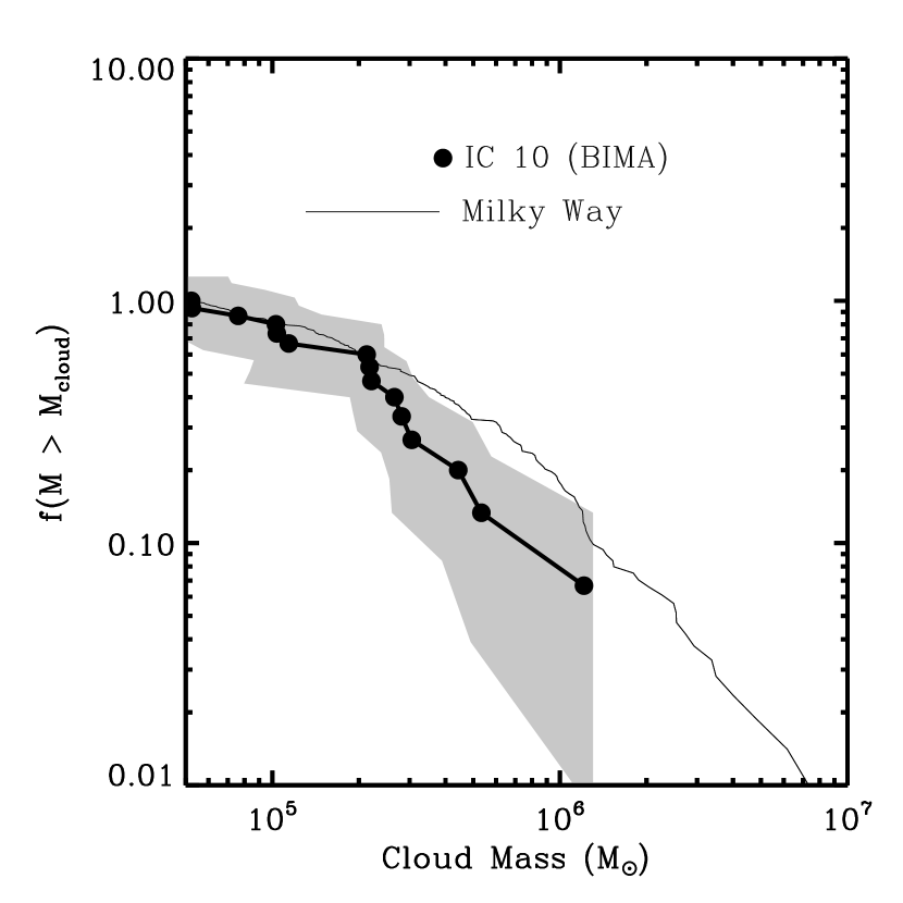
Figure 10.— The cumulative distribution function for GMCs in the Milky Way (solid line) and IC 10 (black circles). We include only Milky Way clouds with $M>10^{5}M_{\odot}$ (the approximate sensitivity of our survey). The gray region shows the area of $1\sigma$ uncertainty, but systematic effects from the identification of clouds are also more important and are not shown.

5.5. CO and H I

The GMCs in IC 10 are found almost exclusively in high column density atomic gas filaments. Figure 4 shows that we find molecular gas only where we find atomic gas, usually above a surface density of $\Sigma_{HI}=10$ M_⊙ pc^-2 ($N(\mbox{\rm{H~{}I}})=1.25\times 10^{21}$ cm^-2). Figure 11 shows the relationship quantitatively, plotting the fraction of the total CO emission as a function H I column density along the line of sight (in black) and the fraction of lines of sight with the specified column density that have associated CO emission (in gray). Half of the molecular gas emission comes from regions with H I column densities above $15$ M_⊙ pc^-2 and $85\%$ is found above a contour of $\Sigma_{HI}=10$ M_⊙ pc^-2. A high column of atomic gas is not a sufficient condition, though, as only $30\%$ of the area in IC 10 with $\Sigma_{HI}>10$ M_⊙ pc^-2 has associated molecular gas and only half of the lines of sight with $\Sigma_{HI}=16$ M_⊙ pc^-2 ($N(\mbox{\rm{H~{}I}})=2.0\times 10^{21}$ cm^-2) have associated CO emission. This discrepancy (necessary, but not sufficient) arises mostly as a result of the large region of relatively high column atomic gas to the east of IC 10. This high column gas is mostly devoid of CO emission, harboring only one molecular cloud. Engargiola et al. (2003) found a similar result in their survey of M 33 — the CO emission comes almost exclusively from within the H I filaments but the presence of a filament does not necessarily imply the presence of CO emission. Similar results can be seen comparing CO emission from the LMC to H I (Fukui et al., 1999; Kim et al., 1998). Broadly, this is the same effect seem in many disk galaxies: the H I extends far out into the disk while molecular gas and star formation are relatively centrally confined (e.g. Wong & Blitz, 2002).

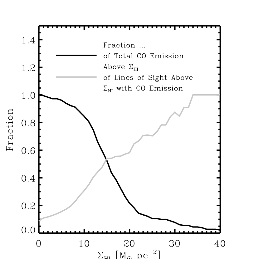
Figure 11.— The fraction of CO emission from IC 10 above a given HI column density, $\Sigma_{HI}$ is shown in black. The fraction of lines of sight with a given HI column density that also show CO emission is shown in gray. Most of the emission comes from regions of the galaxy with column densities above 10 M_⊙ pc^-2, and $50\%$ of the emission arises from regions with $\Sigma_{HI}\gtrsim 16$ M_⊙ pc^-2. Only $50\%$ of lines of sight with this column density has associated molecular gas, however. Although $\Sigma_{HI}\gtrsim 10$ is a necessary condition to find molecular gas, it is not sufficient on its own.

Wong & Blitz (2002) and Blitz & Rosolowsky (2004) have suggested that the hydrostatic gas pressure, $P_{h}$, can predict the ratio of molecular to atomic gas, $f_{mol}=\Sigma_{mol}/\Sigma_{HI}$, over a region of a galaxy. The hydrostatic gas pressure may trace the volume density of gas, $\rho_{gas}$, since $P_{h}=\rho_{gas}~{}v_{g}^{2}$ and the gas velocity dispersion, $v_{g}$, is often quite constant (Blitz & Rosolowsky, 2004, and references therein). The volume density of gas should be more relevant to the formation of H₂ from H I than the surface density. We test whether these arguments hold in IC 10 by calculating $P_{h}$ using the formula derived by Blitz & Rosolowsky (2004) for a stellar-dominated disk,

$$P_{h}=0.84(G\Sigma_{*})^{0.5}\Sigma_{g}\frac{v_{g}}{(h_{*})^{0.5}}\$$ (4)

where $\Sigma_{g}$ is the total surface density of the gas, $\Sigma_{*}$ is the surface density of stars, $v_{g}$ is the velocity dispersion of the gas, and $h_{*}$ is the scale height of the stellar disk. From the H I cube (Wilcots & Miller, 1998), we measured the median $v_{g}$ across the disk (for lines of sight with non-negligible H I emission) to be $\approx 7.5$ km s^-1. We assume the scale height of stars to be comparable to that of disk galaxies ($\sim 300$ pc, see Blitz & Rosolowsky, 2004) and calculate $f_{mol}$ using $X_{CO}=2\times 10^{20}$ cm^-2 (K km s^-1)^-1 (appropriate to the GMCs but perhaps not diffuse gas, see §5.2).

Figure 12 shows reasonable agreement between the IC 10 data and an extrapolation from the Blitz & Rosolowsky (2005) galaxies to low pressure. $P_{h}$ and $f_{mol}$ have a rank correlation coefficient of $0.7\pm 0.1$. The median ratio, $P_{0}=\frac{P_{h}}{f_{mol}}$, is $7\times 10^{4}~{}k_{B}$ and is uncertain by a factor of two. This value of $P_{0}$ (the pressure for which $f_{mol}=1$) is consistent with the results of Blitz & Rosolowsky (2005), who find $P_{0}=4\times 10^{4}~{}k_{B}$ and a nearly linear best fit relation. On average IC 10 is poorer in molecular gas than one might expect by about a factor of two (it lies just under the best fit line from Blitz & Rosolowsky, 2005). Since we used the BIMA survey in this comparison, the discrepancy might be almost completely negated by including the resolved out flux.

Table 8 shows that the pressure is a better predictor of $f_{mol}$ than either the atomic gas surface density or the stellar surface density. The rank correlation between $P_{h}$ and $f_{mol}$ is $0.7\pm 0.1$, higher than the rank correlation between $f_{mol}$ and either $\Sigma_{HI}$ or $\Sigma_{*}$. Both $\Sigma_{HI}$ and $P_{h}$ are very highly correlated with $\Sigma_{mol}$, which demonstrates that the conclusion of Blitz & Rosolowsky (2005) seems to hold in IC 10: H I is a necessary prerequisite for the presence of molecular gas, but not the best predictor of the ratio of molecular to atomic gas. The hydrostatic gas pressure offers an improved prediction of the ratio of molecular to atomic gas because the gravitational influence of a stellar potential well is necessary to enable the formation of H₂ out of H I filaments.

Table 8 Rank Correlations with Molecular to Gas Content

Property	Rank Correlation with $\Sigma_{mol}$	Rank Correlation with $\Sigma_{mol}$/$\Sigma_{HI}$
$\Sigma_{HI}$	$0.6\pm 0.1$	$0.4\pm 0.1$
$\Sigma_{*}$	$0.4\pm 0.1$	$0.5\pm 0.1$
$P_{h}$	$0.8\pm 0.1$	$0.7\pm 0.1$

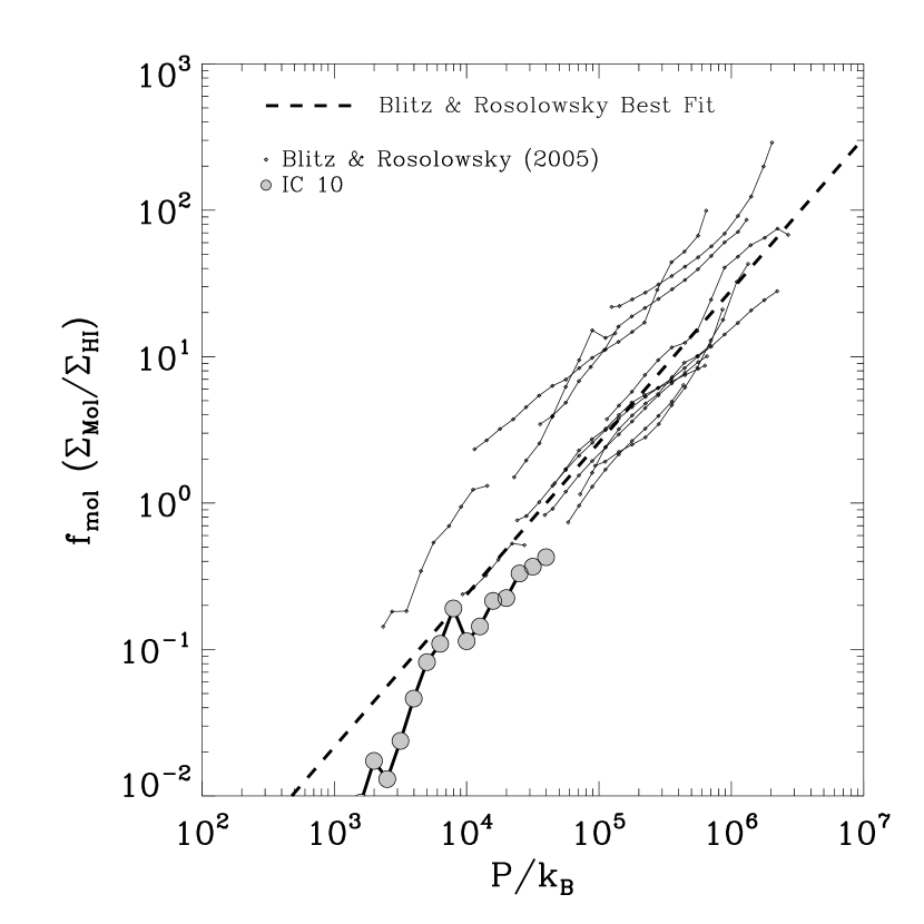
Figure 12.— The molecular-to-atomic ratio plotted as a function of midplane pressure in IC 10. Results and the best fit relation for spiral galaxies from Blitz & Rosolowsky (2005) are shown for comparison. We bin data with similar pressures along lines of sight with $\Sigma_{*}>50$ M_⊙ pc^-2, where the disk approximation may be valid, and apply an inclination correction of $0.67$.

5.6. Star Formation and Gas in IC 10

We showed above that GMCs in IC 10 are similar to those in the Milky Way, M 31, and M 33. Does the molecular gas also form stars at the same rate as molecular gas in spirals? In this section we compare the star formation efficiency (SFR per unit gas) in IC 10 to that in larger galaxies. We perform these comparisons using the H I, CO, and H$\alpha$ maps convolved to a common spatial resolution of $275$ pc ($60^{\prime\prime}$, with $30^{\prime\prime}$ pixels). This is comparable to the scale height of the stellar disk in a spiral galaxy, so we expect the averaging to occur over roughly the same distance along the line of sight and perpendicular to the line of sight. We limit ourselves to regions of the stellar disk of IC 10 with stellar surface densities in excess of $\Sigma_{*}\sim 50$ M_⊙ pc^-2 (obtained from the $K$-band light), because outside this region the three dimensional structure of the H I envelope is uncertain and it is unclear how to interpret the line of sight surface densities.

For galaxies the size of the LMC or bigger, the efficiency with which stars form from molecular gas (and its inverse, the molecular gas depletion time) depends wealky on galaxy mass and Hubble type (Young & Scoville, 1991; Young et al., 1995; Murgia et al., 2002; Leroy et al., 2005). Figure 13 shows the relationship between surface density of star formation and molecular gas surface density for a range of galaxies. Both dwarf galaxies and spirals obey a power law relationship of roughly

$$\Sigma_{SFR}=10^{-3.4\pm 0.1}\Sigma_{Mol}^{1.3\pm 0.1}\mbox{ ,}$$ (5)

where $\Sigma_{SFR}$ is the star formation surface density in units of M_⊙ yr^-1 kpc^-2 and $\Sigma_{Mol}$ is the molecular gas surface density in units of M_⊙ pc^-2(Murgia et al., 2002; Leroy et al., 2005). Figure 13 also shows that IC 10 very clearly does not fall on this trend. Rather, the data for IC 10 show much larger rates of star formation per unit molecular gas than is found in other galaxies — a median factor of $270$ higher. IC 10 is not unique in this regard: both the SMC (Mizuno et al., 2001; Wilke et al., 2004) and the nearby starburst NGC 1569 also show higher SFR surface densities than their CO content would suggest unless X_CO is considerably larger than Galactic in these sources.

The total gas surface density, rather than the H₂ surface density, is often used as a predictor of the star formation. Kennicutt (1998) found that a single power law described the relationship total gas surface density and the star formation surface density across a wide range of galaxies. Data from that paper are plotted along with gas surface densities and H$\alpha$ derived star formation surface densities (SFSDs) in Figure 14. Figure 14 shows that in IC 10, the highest gas surface densities do roughly correspond to the highest star formation rates, although the agreement with Kennicutt (1998) is poor. In particular, regions of high SFSD seem to have lower gas surface densities in IC 10 than galaxies with the same SFSD from the Kennicutt (1998) sample. Furthermore, the scatter in SFSD for a given total gas surface density is very large, particularly around $\Sigma_{HI+H2}\approx 7$ M_⊙ pc^-2.

How can we explain the extremely high efficiency of star formation in IC 10 given the similarity between its GMC properties and those of spiral GMCs? We suggest several possibilities.

1. IC 10 has much more molecular gas than we infer from the CO. The discrepancy between IC 10 and large galaxies may be entirely explained away by a factor of $\sim 30$ increase in the CO-to-H₂ conversion factor. We have presented evidence above that BIMA may resolve out as much flux as it recovers (leaving us with only a factor of $\sim 15$ discrepancy), but the GMC properties we measured above suggest values of $X_{CO}$ that are nearly Galactic. Adjusting the data in Figures 13 and 14 to agree with other galaxies requires more than just a large reservoir of hidden molecular gas; despite producing relatively small amounts of CO emission, this molecular gas must be associated with star formation. It is unlikely that the physical conditions in a hidden reservoir of H₂ could simultaneously be conducive to star formation, inhospitable to CO, and not contribute to the virial masses of the GMCs.

2. The star formation rate of IC 10 is lower than we estimate from the H$\alpha$ due to line-blanketing effects in stellar atmospheres. These effects would cause us to underpredict the UV radiation generated per star, leading to an overestimate of the star formation rate. Studying a sample of stars in the SMC, Massey et al. (2005) found that O stars in that system (with $Z\sim 0.1Z_{\odot}$) had effective temperatures $\sim 4000$ K higher than their solar metallicity analogues. For an O5 star ($T_{eff}\sim 45,000$), this results in the SMC star producing $\sim 50\%$ more ionizing photons. A similar result is obtained using population synthesis codes such as STARBURST99 (Figure 78 in Leitherer et al., 1999) — a shift of an order of magnitude in metallicity for a continuously star forming system results in an increase of $\sim 50\%$ in the number of ionizing photons produced. These adjustments are not large enough to make a significant dent in the discrepancy between IC 10 and larger galaxies.

3. If IC 10 has an unexpectedly top heavy IMF our inferred star formation rates may be too high. Kennicutt et al. (1994) explores the effect of adopting other (Milky Way) IMFs (such as those of Scalo (1986) or Kroupa et al. (1993)) and finds increases of a factor of $\sim 2-3$ to the star formation rate per unit H$\alpha$ emission. A very top-heavy IMF, by contrast, would have the effect of lowering the amount of star formation per unit H$\alpha$ luminosity. The lion’s share of ionizing photons are produced by stars with $M>10$ M_⊙. For the Salpeter IMF assumed in the H$\alpha$ calculation (Kennicutt et al., 1994), $\sim 10\%$ of the mass of stars resides in stars with $M>10$ M_⊙. If IC 10 produced only these stars then the star formation efficiency might be a factor of 10 lower than the value we calculate here. A very top heavy IMF could also explain the unusually high abundance of Wolf Rayet stars in IC 10. However, an IMF that is dramatically skewed towards high masses would contradict the finding by Hunter (2001) that the clusters in IC 10 are consistent with a Galactic IMF. Barring such a dramatic IMF, it seems unlikely that the offset we observe is only a result of a miscalibration of H$\alpha$ as a star formation tracer.

4. The star formation rate in IC 10 may have been higher in the recent past. If IC 10 has recently undergone a period of intense star formation and is now forming stars at (relatively) more modest rate, we may be catching it at a point its life-cycle during which it is (relatively) depleted in molecular gas but still showing the signs of a recent star burst. This scenario could also explain the very high WR star counts and perhaps the discrepancy between the various star formation tracers. In this case, IC 10’s high star formation efficiency may be temporary, an artifact of when we are observing the galaxy. In such a case we would expect a large sample of IC 10-like dwarfs to average to a position consistent with the other galaxies in figures 13 and 14. The higher star formation rate must have occurred within the last $\sim 10$ Myr because high mass stars formed during the period of higher SFR must still be contributing UV photons that create the H$\alpha$ flux. This is consistent with the ages of the clusters found by Hunter (2001), 4 – 30 Myr.

5. Finally, the efficiency of star formation within molecular clouds may indeed be higher in IC 10 than in the Milky Way or other galaxies. This result seems to contradict the similarities between GMCs in IC10 and those in M 31, M 33, and the Milky Way. However, we have emphasized the environmental differences between IC 10 and these systems and these differences may be manifesting themselves in an unexpected way that dramatically affects the efficiency with which molecular gas forms stars.

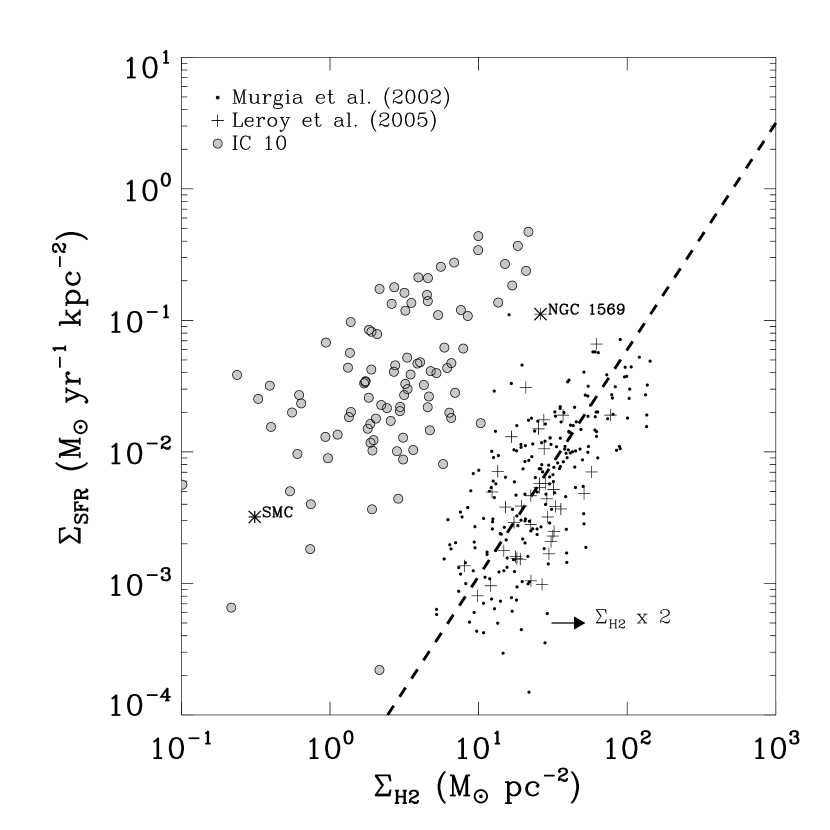
Figure 13.— Star formation surface density as a function of H₂ surface density in IC 10. Global values for large galaxies (Murgia et al., 2002) and LMC-size dwarfs (Leroy et al., 2005) are shown for comparison. We convolve the data to a resolution of $1^{\prime}$ (275 pc) and apply an inclination correction of $0.67$. We plot only points in the stellar disk of IC 10, where $\Sigma_{*}>50$ M_⊙ pc^-2. IC 10 has much more star formation per unit molecular gas than most spirals or dwarfs. We highlight two other dwarfs similar to IC 10: NGC 1569 and the SMC.

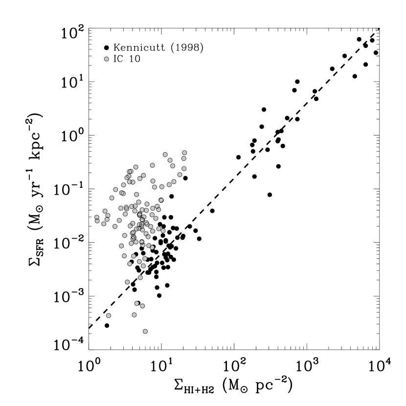
Figure 14.— The Schmidt Law in IC 10. The points and relation of Kennicutt (1998) are shown for comparison. The data have been convolved to a resolution of $1^{\prime}$ (275 pc) and an inclination correction of $0.67$ is applied. We plot only points in the stellar disk of IC 10, where $\Sigma_{*}>50$ M_⊙ pc^-2. IC 10 shows more star formation per unit gas than large galaxies.

6. Summary and Conclusions

We present a complete survey ¹²CO $J=$($1\rightarrow 0$) in IC 10 using BIMA. The survey covers all of the optical disk of IC 10 and a large part of the extended H I structure with a resolution of $14^{\prime\prime}$ (70 pc) and a sensitivity sufficient to detect clouds with masses greater than $4\times 10^{4}$ M_⊙. We find structures across the optical disk of the galaxy and in the extended structure to the north and east of the galaxy. The BIMA finds a total CO luminosity of $1.0\times 10^{6}$ K km s^-1 pc².

We also present ARO 12m observations of 22 fields in IC 10, corresponding to most of the locations in which CO emission is detected by the BIMA survey and a number of locations of interest with no CO emission. The ARO 12m detects CO emission only where BIMA also detects CO emission. The ARO 12m finds more emission than BIMA or OVRO along the same line of sight. This may be evidence for an extended CO component surrounding the more compact structures detected by the interferometers. Comparing the integrated luminosity from the ARO 12m to the BIMA survey, we estimate that the true CO luminosity of IC 10 is $2.2\times 10^{6}$ K km s^-1 pc².

We measure the properties of 14 resolved CO structures in IC 10 from high resolution OVRO data by Walter (2003). The sizes, line widths, and luminosities of these structures resemble those of GMCs found in similar surveys of M 31, M 33 (Rosolowsky et al., 2003; Rosolowsky & Leroy, 2005), and Milky Way GMCs (Solomon et al., 1987). We conclude that we are observing GMCs in IC 10. The virial-mass to luminosity ratio in these GMCs is comparable to that observed for spiral galaxy GMCs and we argue that this implies that a Galactic CO-to-H₂ conversion factor applies to IC 10. We can not constrain the conversion factor in the gas resolved out by the interferometers.

Most of the CO emission detected by the BIMA survey comes from lines of sight with $\Sigma_{HI}$ above 10 M_⊙ pc^-2 ($N(\mbox{\rm{H~{}I}})=1.25\times 10^{21}$ cm^-2) and all of the CO emission is very close to such regions. However, only 30$\%$ of the lines of sight with $\Sigma_{HI}>10$ M_⊙ pc^-2 have associated CO emission. This may be because not all high column density H I actually corresponds to high volume density gas. Indeed, we show that hydrostatic gas pressure predicts the CO along a line of sight better than the H I column alone. Further, the ratio of molecular to atomic gas along a line of sight obeys the same simple relationship in IC 10 that is seen in large spiral galaxies.

IC 10 displays significantly more star formation (H$\alpha$) for a given gas surface density (molecular or total) than large spiral galaxies. We suggest several explanations for this: a higher CO-to-H₂ conversion factor, a different IMF or SFR calibration, or a biased (in time) perspective. The last explanation is appealing — namely that IC 10’s unusual star formation efficiency is a timing effect. We may be observing a starburst just past its peak, so that the signatures of star formation are still present but the star-forming gas has already been somewhat depleted.

References

- Becker (1990) Becker, R., Ph. D. Thesis, University of Bonn
- Bell (2003) Bell, E. F. 2003, ApJ, 586, 794
- Blitz (1985) Blitz, L. 1985, ApJ, 296, 481
- Blitz & Rosolowsky (2004) Blitz, L., & Rosolowsky, E. 2004, ApJ, 612, L29
- Blitz & Rosolowsky (2005) Blitz, L., & Rosolowsky, E. 2005, in preparation.
- Bohlin et al. (1978) Bohlin, R. C., Savage, B. D., & Drake, J. F. 1978, ApJ, 224, 132
- Bolatto et al. (2000) Bolatto, A. D., Jackson, J. M., Wilson, C. D., & Moriarty-Schieven, G. 2000, ApJ, 532, 909
- Bolatto et al. (2003) Bolatto, A. D., Leroy, A., Israel, F. P., & Jackson, J. M. 2003, ApJ, 595, 167
- Borissova et al. (2000) Borissova, J., Georgiev, L., Rosado, M., Kurtev, R., Bullejos, A., & Valdez-Gutiérrez, M. 2000, A&A, 363, 130
- Bot et al. (2004) Bot, C., Boulanger, F., Lagache, G., Cambrésy, L., & Egret, D. 2004, A&A, 423, 567
- Calzetti et al. (1994) Calzetti, D., Kinney, A. L., & Storchi-Bergmann, T. 1994, ApJ, 429, 582
- Cardelli et al. (1989) Cardelli, J. A., Clayton, G. C., & Mathis, J. S. 1989, ApJ, 345, 245
- Crowther et al. (2003) Crowther, P. A., Drissen, L., Abbott, J. B., Royer, P., & Smartt, S. J. 2003, A&A, 404, 483
- Dame et al. (2001) Dame, T. M., Hartmann, D., & Thaddeus, P. 2001, ApJ, 547, 792
- de Vaucouleurs et al. (1991) de Vaucouleurs, G., de Vaucouleurs, A., Corwin, H. G., Buta, R. J., Paturel, G., & Fouque, P. 1991, S&T, 82, 621
- Dufour (1984) Dufour, R. J. 1984, IAU Symp. 108: Structure and Evolution of the Magellanic Clouds, 108, 353
- Engargiola et al. (2003) Engargiola, G., Plambeck, R. L., Rosolowsky, E., & Blitz, L. 2003, ApJS, 149, 343
- Fukui et al. (1999) Fukui, Y., et al. 1999, PASJ, 51, 745
- Garnett (1990) Garnett, D. R. 1990, ApJ, 363, 142
- Gil de Paz et al. (2003) Gil de Paz, A., Madore, B. F., & Pevunova, O. 2003, ApJS, 147, 29
- Greggio et al. (1998) Greggio, L., Tosi, M., Clampin, M., de Marchi, G., Leitherer, C., Nota, A., & Sirianni, M. 1998, ApJ, 504, 725
- Greve et al. (1996) Greve, A., Becker, R., Johansson, L. E. B., & McKeith, C. D. 1996, A&A, 312, 391
- Helfer et al. (2002) Helfer, T. T., Vogel, S. N., Lugten, J. B., & Teuben, P. J. 2002, PASP, 114, 350
- Huchtmeier & Richter (1988) Huchtmeier, W. K., & Richter, O.-G. 1988, A&A, 203, 237
- Hunter (2001) Hunter, D. A. 2001, ApJ, 559, 225
- Hunter et al. (2001) Hunter, D. A., et al. 2001, ApJ, 553, 121
- Israel (1988) Israel, F. P. 1988, A&A, 194, 24
- Israel (1997) Israel, F. P. 1997, A&A, 328, 471
- Israel (1997) Israel, F. P. 1997, A&A, 317, 65
- Jarrett et al. (2003) Jarrett, T. H., Chester, T., Cutri, R., Schneider, S. E., & Huchra, J. P. 2003, AJ, 125, 525
- Kennicutt et al. (1994) Kennicutt, R. C., Tamblyn, P., & Congdon, C. E. 1994, ApJ, 435, 22
- Kennicutt (1998) Kennicutt, R. C. 1998, ApJ, 498, 541
- Kim et al. (1998) Kim, S., Staveley-Smith, L., Dopita, M. A., Freeman, K. C., Sault, R. J., Kesteven, M. J., & McConnell, D. 1998, ApJ, 503, 674
- Kroupa et al. (1993) Kroupa, P., Tout, C. A., & Gilmore, G. 1993, MNRAS, 262, 545
- Larson (1981) Larson, R. B. 1981, MNRAS, 194, 809
- Leitherer et al. (1999) Leitherer, C., et al. 1999, ApJS, 123, 3
- Leroy et al. (2005) Leroy, A., Bolatto, A. D., Simon, J. D., & Blitz, L. 2005, ApJ, 625, 763
- Lequeux et al. (1979) Lequeux, J., Peimbert, M., Rayo, J. F., Serrano, A., & Torres-Peimbert, S. 1979, A&A, 80, 155
- Madden et al. (1997) Madden, S. C., Poglitsch, A., Geis, N., Stacey, G. J., & Townes, C. H. 1997, ApJ, 483, 200
- Maeder & Conti (1994) Maeder, A., & Conti, P. S. 1994, ARA&A, 32, 227
- Massey & Armandroff (1995) Massey, P., & Armandroff, T. E. 1995, AJ, 109, 2470
- Massey & Holmes (2002) Massey, P., & Holmes, S. 2002, ApJ, 580, L35
- Massey et al. (2003) Massey, P., Olsen, K. A. G., & Parker, J. W. 2003, PASP, 115, 1265
- Massey et al. (2005) Massey, P., Puls, J., Pauldrach, A. W. A., Bresolin, F., Kudritzki, R. P., & Simon, T. 2005, ApJ, 627, 477
- Mateo (1998) Mateo, M. L. 1998, ARA&A, 36, 435
- Melisse & Israel (1994) Melisse, J. P. M. & Israel, F. P. 1994, A&AS, 103, 391
- Mizuno et al. (2001) Mizuno, N., Rubio, M., Mizuno, A., Yamaguchi, R., Onishi, T., & Fukui, Y. 2001, PASJ, 53, L45
- Murgia et al. (2002) Murgia, M., Crapsi, A., Moscadelli, L., & Gregorini, L. 2002, A&A, 385, 412
- Ohta et al. (1988) Ohta, K., Sasaki, M., & Saito, M. 1988, PASJ, 40, 653
- Ohta et al. (1992) Ohta, K., Sasaki, M., Yamada, T., Saito, M., & Nakai, N. 1992, PASJ, 44, 585
- Polk et al. (1988) Polk, K. S., Knapp, G. R., Stark, A. A., & Wilson, R. W. 1988, ApJ, 332, 432
- Richer & McCall (1995) Richer, M. G. & McCall, M. L. 1995, ApJ, 445, 642
- Rosolowsky et al. (2003) Rosolowsky, E., Engargiola, G., Plambeck, R., & Blitz, L. 2003, ApJ, 599, 258
- Rosolowsky (2005) Rosolowsky, E. 2005, ApJ submitted.
- Rosolowsky & Leroy (2005) Rosolowsky, E. & Leroy, A. 2005, in prep.
- Sakai et al. (1999) Sakai, S., Madore, B. F., & Freedman, W. L. 1999, ApJ, 511, 671
- Scalo (1986) Scalo, J. M. 1986, Fundamentals of Cosmic Physics, 11, 1
- Schlegel et al. (1998) Schlegel, D. J., Finkbeiner, D. P., & Davis, M. 1998, ApJ, 500, 525
- Shostak & Skillman (1989) Shostak, G. S., & Skillman, E. D. 1989, A&A, 214, 33
- Simon et al. (2005) Simon, J. D., Bolatto, A. D., Leroy, A., Blitz, L., & Gates, E. L. 2005, ApJ, 621, 757
- Solomon et al. (1987) Solomon, P. M., Rivolo, A. R., Barrett, J., & Yahil, A. 1987, ApJ, 319, 730
- Stanimirović et al. (2000) Stanimirovic, S., Staveley-Smith, L., van der Hulst, J. M., Bontekoe, T. R., Kester, D. J. M., & Jones, P. A. 2000, MNRAS, 315, 791
- Stanimirović, Staveley-Smith, & Jones (2004) Stanimirović, S., Staveley-Smith, L., & Jones, P. A. 2004, ApJ, 604, 176
- Strong & Mattox (1996) Strong, A. W., & Mattox, J. R. 1996, A&A, 308, L21
- Taylor et al. (1999) Taylor, C. L., Hüttemeister, S., Klein, U., & Greve, A. 1999, A&A, 349, 424
- Thronson et al. (1990) Thronson, H. A., Hunter, D. A., Casey, S., & Harper, D. A. 1990, ApJ, 355, 94
- Walter (2003) Walter, F., 2003, Proceedings of the 4th Cologne-Bonn Zermatt Symposium ”The Dense Interstellar Medium in Galaxies”
- Welch et al. (1996) Welch, W. J., et al. 1996, PASP, 108, 93
- White & Becker (1992) White, R. L., & Becker, R. H. 1992, ApJS, 79, 331
- Wilke et al. (2004) Wilke, K., Klaas, U., Lemke, D., Mattila, K., Stickel, M., & Haas, M. 2004, A&A, 414, 69
- Wilcots & Miller (1998) Wilcots, E. M., & Miller, B. W. 1998, AJ, 116, 2363
- Wilson & Reid (1991) Wilson, C. D., & Reid, I. N. 1991, ApJ, 366, L11
- Wilson (1995) Wilson, C. D. 1995, ApJ, 448, L97
- Wolfire et al. (1995) Wolfire, M. G., Hollenbach, D., McKee, C. F., Tielens, A. G. G. M., & Bakes, E. L. O. 1995, ApJ, 443, 152
- Wong & Blitz (2002) Wong, T., & Blitz, L. 2002, ApJ, 569, 157
- Yang & Skillman (1993) Yang, H., & Skillman, E. D. 1993, AJ, 106, 1448
- Young & Scoville (1991) Young, J. S. & Scoville, N. Z. 1991, ARA&A, 29, 581
- Young et al. (1995) Young, J. S., et al. 1995, ApJS, 98, 219