Turbulence from localized random expansion waves

Abstract

In an attempt to determine the outer scale of turbulence driven by localized sources, such as supernova explosions in the interstellar medium, we consider a forcing function given by the gradient of gaussian profiles localized at random positions. Different coherence times of the forcing function are considered. In order to isolate the effects specific to the nature of the forcing function we consider the case of a polytropic equation of state and restrict ourselves to forcing amplitudes such that the flow remains subsonic. When the coherence time is short, the outer scale agrees with the half-width of the gaussian. Longer coherence times can cause extra power at large scales, but this would not yield power law behavior at scales larger than that of the expansion waves. At scales smaller than the scale of the expansion waves the spectrum is close to power law with a spectral exponent of $-2$. The resulting flow is virtually free of vorticity. Viscous driving of vorticity turns out to be weak and self-amplification through the nonlinear term is found to be insignificant. No evidence for small scale dynamo action is found in cases where the magnetic induction equation is solved simultaneously with the other equations.

1 Introduction

Turbulence plays an important role in many branches of astrophysics. During the past decade simulations have been employed to address fundamental questions in turbulent stellar convection zones (Spruit, Nordlund, & Title, 1990), accretion discs (Balbus & Hawley, 1998), and interstellar turbulence (Korpi et al., 1999a; Balsara et al., 2004; Dib et al., 2006). In these three cases the nature of energy injection is quite different; convective instability, magneto-rotational instability, and explicit driving through supernova explosions, respectively. Nevertheless, important insights into the nature of astrophysical turbulence have been obtained by studying turbulence forced on large scales by adding random time-dependent large scale perturbations to the velocity. This allows the study of the turbulent cascade of kinetic energy from large scales to smaller scales, and eventually down to the dissipative scale (see, e.g., Brandenburg & Subramanian, 2005, for a review). While the scale of the aforementioned instabilities can indeed be large (comparable with the system size), this is not so evident in the case of random forcing by supernova explosions. The energy released by supernova explosions, and to a lesser extend also by stellar winds and outflows, suffices to power interstellar turbulence (Vázquez-Semadeni, Passot, & Pouquet, 1996). The anticipated outer scale of the turbulence is around 100 pc (e.g., Beck et al., 1996). This is large compared with the size of individual supernova explosion sites. Some supernova remnants can stay reasonably coherent for scales up to several tens of parsec. Furthermore, supernova explosions are known to be clustered, forming thereby large expanding patches called superbubbles (e.g., Norman & Ikeuchi, 1989; Ferrière, 1992). Their scale is often larger than the scaleheight of the galactic disc, and they are primarily responsible for driving fountain-like outflows. In any case, it appears that the localized point-like supernova explosions are able to act as a driver of the turbulence on a much larger scale.

An obvious question concerns the connection between the artificial forcings assumed in many computer simulations and any of the more realistic types of forcing. In the present paper we consider the properties of turbulence driven by random, localized expansion waves, mimicking certain aspects of supernova-driven explosions. One of the questions we are able to address with such a setup concerns information about the scale of the energy-carrying eddies of turbulence that is driven by small localized expansion waves. Is it true that such localized energy injections produce kinetic energy predominantly at the scale of the original expansion wave, even though this scale is in general quite small? What are the effects, if any, that could shift the dominant power to larger scales. Large scales might plausibly arise if the duration of energy injection at one particular site becomes comparable to or larger than the turnover time of the resulting turbulence. This would reinforce the original expansion wave until it has grown to a larger size. These issues are not directly connected with compressibility or with the effects of cooling or the nature of the equation of state of the gas. Thus, although interstellar turbulence is certainly highly supersonic, we consider here the case of subsonic turbulence in order to make the connection between solenoidal forcing in the form of plane waves and irrotational forcing driving localized expansion waves.

2 Method

We solve the compressible Navier-Stokes equations assuming a polytropic equation of state relating the pressure $p$ to the density $\rho$ via $p=K\rho^{\gamma}$ with $\gamma=5/3$ and polytropic coefficient $K=c_{\rm s0}^{2}/(\gamma\rho_{0}^{\gamma-1})$, where $c_{\rm s0}$ and $\rho_{0}$ are constants. The momentum equation can then be written in the form

$$\frac{{\rm D}{}{\bm{u}}}{{\rm D}{}t}=-\mbox{\boldmath$\nabla$}{}h+\mbox{\boldmath$f$}{}+{\bm{F}}_{\rm visc},$$ (1)

where

$$h={\rho_{0}c_{\rm s0}^{2}\over\gamma-1}\left({\rho\over\rho_{0}}\right)^{\gamma-1}$$ (2)

is the enthalpy, ${\rm D}{}/{\rm D}{}t=\partial/\partial t+{\bm{u}}\cdot\mbox{\boldmath$\nabla$}{}$ is the advective derivative, and ${\bm{F}}_{\rm visc}=\rho^{-1}\mbox{\boldmath$\nabla$}{}\cdot\left(2\rho\nu\mbox{\boldmath$\sf S$}{}\right)$ is the viscous force, where ${\sf S}_{ij}=\frac{1}{2}(u_{i,j}+u_{j,i})-\frac{1}{3}\delta_{ij}\mbox{\boldmath$\nabla$}{}\cdot{\bm{u}}$ is the traceless rate of strain tensor. The density obeys the continuity equation,

$$\frac{{\rm D}{}\ln\rho}{{\rm D}{}t}=-\mbox{\boldmath$\nabla$}{}\cdot{\bm{u}}.$$ (3)

We adopt a gaussian potential forcing function $f$ of the form

$$\mbox{\boldmath$f$}{}({\bm{x}},t)=\mbox{\boldmath$\nabla$}{}\phi$$ (4)

with

$$\phi({\bm{x}},t)=N\exp\left\{[{\bm{x}}-{\bm{x}}_{\rm f}(t)]^{2}/R^{2}\right\},$$ (5)

where ${\bm{x}}=(x,y,z)$ is the position vector, ${\bm{x}}_{\rm f}(t)$ is the random forcing position, $R$ is the radius of the gaussian, and $N$ is a normalization factor. We consider two forms for the time dependence of ${\bm{x}}_{\rm f}$. First, we take ${\bm{x}}_{\rm f}$ such that the forcing is $\delta$-correlated in time. Second, we include a forcing time ${\delta{}t}_{\rm force}$ that defines the interval during which ${\bm{x}}_{\rm f}$ remains constant. On dimensional grounds the normalization is chosen to be $N=c_{\rm s0}\sqrt{c_{\rm s0}R/\Delta{}t}$, where

$$\Delta{}t=\max\left(\delta{}t,\delta{}t_{\rm force}\right)$$ (6)

is the length of the time step, $\delta t$, in the $\delta$-correlated case or equal to the mean interval $\delta{}t_{\rm force}$ during which the force remains unchanged, depending on which is longer. We begin by considering the nature of flows generated in each case in the absence of a magnetic field. We use the Pencil Code, which is a non-conservative, high-order, finite-difference code (sixth order in space and third order in time) for solving the compressible hydrodynamic and hydromagnetic equations. We adopt non-dimensional variables by measuring speed in units of the sound speed, $c_{\rm s0}$, and length in units of $1/k_{1}$, where $k_{1}$ is the smallest wavenumber in the periodic domain. This implies that the nondimensional size of the domain is $(2\pi)^{3}$.

3 Results

3.1 Delta-correlated forcing function

We begin with the case where $\delta t_{\rm force}=0$, so the forcing function is $\delta$-correlated in time. In Figs 1 and 2 we show the resulting time averaged energy spectra for two different resolutions. The results are relatively robust with respect to changes in the resolution. Also, the spectra are found to converge quite quickly after only about 5–7 turnover times, suggesting that there are no strong transients. For the results presented below, the durations of the runs, $T_{\rm run}$, is given in terms of the turnover time,

$$N_{\rm turn}=u_{\rm rms}k_{\rm peak}T_{\rm run},$$ (7)

where $k_{\rm peak}$ is the effective forcing wavenumber which, in turn, depends on the radius of the initial expansion wave, $R$. Indeed, the energy spectra show maximum power at the wavenumber $k_{\rm peak}$, which is approximately inversely proportional to $R$, with

$$k_{\rm peak}R\approx 2.$$ (8)

The wavenumber $k_{\rm peak}$ agrees with the width of the Fourier-transformed forcing function. [Note that the Fourier transform of $\exp(-x^{2}/R^{2})$ is $\exp(-k^{2}R^{2}/4)$.] This result is therefore not surprising, but it confirms quite clearly that a $\delta$-correlated forcing function consisting of localized expansion waves produces maximum energy injections at the scale of the expansion wave itself. This would therefore not explain the energy spectrum seen for example in simulations of supersonic turbulence (Porter et al., 1998; Padoan & Nordlund, 1999; Haugen et al., 2004) or those inferred for interstellar turbulence (Han et al., 2004), where energy injection is assumed to occur at the scale of the domain.

Figure 1: Time averaged energy spectra for $R=0.2$ (dotted line), 0.5 (dashed line), and 1 (solid line). The durations of the runs are $N_{\rm turn}=333$, 224, and 81 turnover times, respectively. $128^{3}$ mesh points, $\nu=10^{-3}$, and $\delta$-correlated forcing. The vertical arrows indicate the effective forcing wavenumber, as obtained from Eq. (8).

Figure 2: Same as Fig. 1, but for $256^{3}$ mesh points, $\nu=5\times 10^{-4}$, for $R=0.2$ (dotted line), 0.5 (dashed line), and 1 (solid line). The durations of the runs are $N_{\rm turn}=120$, 64, and 29 turnover times, respectively.

The energy spectrum shows a distinct $k^{-2}$ subrange. Such a slope is predicted for shock turbulence (Kadomtsev & Petviashvili, 1973), although here the flow is subsonic and without shocks. However, it may be interesting to note that a $k^{-2}$ spectrum has also been seen in the irrotational component of transonic turbulence (Porter et al., 1998). Energetically, the irrotational component is subdominant compared with the solenoidal components (Porter et al., 1998; Padoan & Nordlund, 1999; Haugen et al., 2004). In the present simulations, however, there is hardly any vorticity and the flow is entirely dominated by the irrotational component. This, in turn, is a consequence of the irrotational nature of the forcing function combined with the fact that the viscosity is low, so that very little vorticity is produced. We consider vorticity production in more detail in Sect. 3.3 below.

3.2 Forcing function with memory

Next we look at the case where the expansion wave persists for a certain amount of time, $\delta t_{\rm force}$. In Fig. 3 we show time averaged spectra for different values of $\delta t_{\rm force}$. This time interval is conveniently expressed in non-dimensional form as a Strouhal number (Landau & Lifshitz, 1987; Krause & Rädler, 1980),

$$\mbox{St}=\delta t_{\rm force}u_{\rm rms}k_{\rm peak}.$$ (9)

Note that for larger values of $\delta t_{\rm force}$ the spectrum consists of separated bumps, but the overall power appears to be shifted to larger scales and smaller wavenumbers. The presence of bumps is suggestive of an acoustic resonance or standing wave pattern that may be excited in the simulation box. Such a phenomenon is unfamiliar in the context of mostly vortical turbulence. It is plausible, and indeed compatible with our as yet limited results, that these bumps can only occur if there is sufficient scale separation between $k_{\rm peak}$ and $k_{1}$. Furthermore, bumps in the spectrum seem to be possible only when the memory time is not too short, i.e. when the effects of temporal randomness are limited.

Figure 3: Time averaged energy spectra for $R=0.2$ for $\delta t_{\rm force}=1$ ($\mbox{St}=0.08$, dashed line), $\delta t_{\rm force}=0.2$ ($\mbox{St}=0.05$, solid line), and $\delta t_{\rm force}=0$ (i.e. $\delta$-correlated, $\mbox{St}=0$, dotted line). The durations of the runs are $N_{\rm turn}=16$, 64, and 333 turnover times, respectively, and the rms velocities are 0.008, 0.027, and 0.058, respectively. $128^{3}$ mesh points, $\nu=10^{-3}$.

In Figs 4 and 5 we demonstrate that decreasing viscosity and increasing resolution produces more power at small scales, gradually building up a $k^{-2}$ power law between the forcing scale and the dissipative cutoff scale when the resolution is sufficient for those scales to be resolved.

Visualizations of the density (Fig. 6) show how the initially highly ordered expansion waves turn rapidly into a complicated pattern. By the time $t=50$ the velocity has reached a statistically steady state and the flow has ceased to bear any resemblance to the initial expansion wave.

Figure 4: Dependence on viscosity. Time averaged energy spectra for $\nu=2\times 10^{-4}$ (solid line), $\nu=5\times 10^{-4}$ (dashed line), $\nu=10^{-3}$ (dotted line). The durations of the runs are $N_{\rm turn}=28$, 17, and 138 turnover times, respectively, and the values of the St are 0.23, 0.19, and 0.17, respectively. $\delta t_{\rm force}=1$, $R=0.2$, $128^{3}$ mesh points.

Figure 5: Dependence on resolution. Time averaged energy spectra for $R=0.2$, using $512^{3}$ mesh points (solid line, $\nu=5\times 10^{-5}$), $256^{3}$ mesh points (dashed line, $\nu=10^{-4}$), and $128^{3}$ mesh points (dotted line, $\nu=2\times 10^{-4}$). The durations of the runs are $N_{\rm turn}=22$, 59, and 28 turnover times, respectively, and the values of St are 0.25, 0.24, and 0.23, respectively. The insets shows the evolution of $u_{\rm rms}$ and $\omega_{\rm rms}$ for the run with $512^{3}$ mesh points.

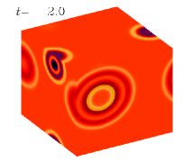
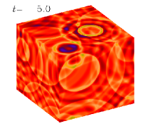
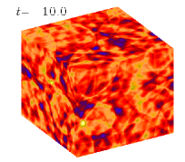
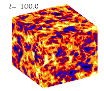
Figure 6: Visualization of $\ln\rho$ on the periphery of the box at different times, for $k_{1}R=0.2$,$\mbox{Re}=50$, $\mbox{St}=0.25$, $\nu=5\times 10^{-5}$, and $512^{3}$ mesh points. Note that in the fully developed state individual expansion waves can hardly be recognized.

3.3 Vorticity production

One of the main differences between the present forcing function and those used in some previous papers (Eswaran & Pope, 1988; Porter et al., 1998; Padoan & Nordlund, 2002; Haugen et al., 2004) is that here the forcing is completely irrotational, i.e. $\mbox{\boldmath$\nabla$}{}\times\mbox{\boldmath$f$}{}=0$ and $\mbox{\boldmath$\nabla$}{}\cdot\mbox{\boldmath$f$}{}\neq 0$. Therefore, unlike previous cases where instead $\mbox{\boldmath$\nabla$}{}\times\mbox{\boldmath$f$}{}\neq 0$ and $\mbox{\boldmath$\nabla$}{}\cdot\mbox{\boldmath$f$}{}=0$, and where vorticity ($\mbox{\boldmath$\omega$}{}=\mbox{\boldmath$\nabla$}{}\times{\bm{u}}$) was immediately produced, here vorticity can only be produced through viscous interactions. This can be seen by writing the viscous force in the form

$${\bm{F}}_{\rm visc}=-\nu\nabla\times\nabla\times{\bm{u}}+{\textstyle{4\over 3}}\nu\mbox{\boldmath$\nabla$}{}\mbox{\boldmath$\nabla$}{}\cdot{\bm{u}}+\nu{\bm{G}},$$ (10)

where $G_{i}={\sf S}_{ij}\nabla_{j}\ln\rho$ is a term that could drive vorticity even with zero vorticity initially. Indeed, the vorticity equation, obtained by taking the curl of Eq. (1), can then be written as

$${\partial\mbox{\boldmath$\omega$}{}\over\partial t}=\mbox{\boldmath$\nabla$}{}\times({\bm{u}}\times\mbox{\boldmath$\omega$}{})+\nu\nabla^{2}\mbox{\boldmath$\omega$}{}+\nu\mbox{\boldmath$\nabla$}{}\times{\bm{G}}.$$ (11)

Note the absence of the baroclinic term, i.e. the cross product of temperature and specific entropy gradients. This is because we have restricted ourselves to a gas with an isothermal equation of state. The baroclinic term is known to produce vorticity (e.g. Korpi et al., 1999b). The nonlinear term, $\mbox{\boldmath$\nabla$}{}\times({\bm{u}}\times\mbox{\boldmath$\omega$}{})$, could in principle lead to exponential amplification of an initial seed vorticity—much like a term in the small scale dynamo problem, discussed in the next section. However, no evidence for such an effect has been found in the present simulations. Thus, the only remaining term is $\mbox{\boldmath$\nabla$}{}\times{\bm{G}}$ which is due to viscosity. One might therefore expect that as we decrease the Reynolds number, defined here in terms of $k_{\rm peak}$ as

$$\mbox{Re}=u_{\rm rms}/\left(\nu k_{\rm peak}\right),$$ (12)

the amount of vorticity production decreases. The numerical simulations yield values for the normalized vorticity,

$$\mbox{normalized vorticity}=\omega_{\rm rms}/(u_{\rm rms}k_{\rm peak}),$$ (13)

that are essentially within the ‘noise’. Indeed, the data shown in Table LABEL:Tsum are well below unity and do not give a clear trend as a function of resolution or Reynolds number. For all these runs the Strouhal number is $\mbox{St}\approx 0.25$.

Table 1: Results for the normalized vorticity, $\omega_{\rm rms}/(u_{\rm rms}k_{\rm peak})$, as a function of Re and resolution. The durations of the runs vary between $N_{\rm turn}=16$ and 250 turnover times, and $\nu$ varies between $10^{-3}$ and $5\times 10^{-5}$. For the high resolution run with $512^{3}$ meshpoints and $\nu=5\times 10^{-5}$ we have $N_{\rm turn}=59$ turnover times.

Re $512^{3}$ $256^{3}$ $128^{3}$ 50 $1.4\times 10^{-3}$ $8.7\times 10^{-3}$ 25 $1.1\times 10^{-2}$ $2.9\times 10^{-3}$ 12 $1.6\times 10^{-2}$ $2.0\times 10^{-3}$ 4 $7.6\times 10^{-3}$ $1.5\times 10^{-3}$

In conclusion, the amount of vorticity production depends mostly on the numerical resolution, suggesting that no measurable vorticity is produced by physical effects.

3.4 Dynamo action?

In view of the formal analogy between the vorticity and induction equations (Batchelor, 1950), it appears that dynamo action should be as difficult to achieve as the amplification of vorticity by the nonlinear term, $\mbox{\boldmath$\nabla$}{}\times({\bm{u}}\times\mbox{\boldmath$\omega$}{})$. In order to address this problem, we solve the induction equation for the magnetic field ${\bm{B}}$,

$${\partial{\bm{B}}\over\partial t}=\mbox{\boldmath$\nabla$}{}\times({\bm{u}}\times{\bm{B}})+\eta\nabla^{2}{\bm{B}},$$ (14)

simultaneously with the other equations. Equation (1) gains a term—the Lorentz force per unit mass, ${\bm{J}}\times{\bm{B}}/\rho$, but this effect would only become important once the magnetic field becomes strong. (Here, ${\bm{J}}=\mbox{\boldmath$\nabla$}{}\times{\bm{B}}/\mu_{0}$ is the current density and $\mu_{0}$ is the vacuum permeability.) As initial condition we adopt a magnetic vector potential that is $\delta$-correlated in space. This results in a magnetic energy spectrum proportional to $k^{4}$.

In all the cases that we have investigated so far, we have not found evidence of field amplification, i.e. there is no dynamo action. Our highest resolution run has $512^{3}$ mesh points and a magnetic Reynolds number, $R_{\rm m}=u_{\rm rms}/(\eta k_{\rm peak})$, of 250 and $\mbox{Re}=50$. Kinetic and magnetic energy spectra are shown in Fig. 7. For this run the magnetic decay rate, $\lambda=-{\rm d}{}\ln B_{\rm rms}/{\rm d}{}t$, is about 30 times the ohmic decay rate, $\eta k_{\rm peak}^{2}$. This is approximately equal to the scale separation ratio between $k_{\rm peak}$ and the dissipative cutoff wavenumber. Such a rapid decay rate suggests that this type of flow has a highly destructive effect on the magnetic field. Energy spectra of the magnetic field confirm that the spectral energy decays at small scales, while it stays unchanged at large scales.

Figure 7: Kinetic and magnetic energy spectra, $E(k)$ and $M(k)$, respectively, at three different times, separated by $\Delta t=20\delta t_{\rm force}$, with for $R=0.2$, $R_{\rm m}=u_{\rm rms}/(\eta k_{\rm peak})=250$, $\mbox{Re}=50$, and $512^{3}$ mesh points. The duration of the run is $N_{\rm turn}=22$ turnover times. $\nu=5\times 10^{-5}$, $\eta=5\times 10^{-5}$.

The absence of any dynamo action agrees with earlier results for purely irrotational turbulence (Brooks, 1999). On the other hand, earlier analytic considerations suggested that dynamo action should be possible for irrotational flows and that the growth rate should increase with increasing Mach number to the fourth power (Kazantsev et al., 1985; Moss & Shukurov, 1996). Subsequent work by Haugen et al. (2004) did not discuss growth rates, but critical magnetic Reynolds numbers which shows that the small scale (non-helical) dynamo becomes about twice as hard to excite when the Mach number exceeds unity. This was explained by the presence of an additional irrotational contribution in the supersonic case. This contribution remained however subdominant and did not contribute to the dynamo. This is consistent with the present result that up to the largest magnetic Reynolds numbers accessible today, purely irrotational turbulence does not produce dynamo action.

4 Conclusion

The localized expansion waves used as forcing functions in the present paper resemble in some ways the driving by supernova explosions. An obvious difference is that the supernova driving produces highly supersonic flows. This may be important in connection with understanding the amount of vorticity production in irrotationally forced flows. Indeed, Korpi et al. (1999b) found that the main driver of vorticity production in their supernova driven turbulence simulations is the baroclinic term.

The present work suggests that the turbulence would indeed be peaked primarily at small scales. Memory effects (i.e. finite values of ${\delta{}t}_{\rm force}$) contribute somewhat to enhancing power at larger scales, but, because of the dip in power at intermediate scales, the resulting energy spectrum is still very different from the power law spectra obtained with forcing directly at large scales. The main difference is the absence of vorticity in the present simulations. Since vorticity is mainly driven by the baroclinic term, we may expect that it is also this term that would primarily contribute to enhanced power at low wave numbers, corresponding to scales larger than the radius of the original expansion waves.

References

- Balbus & Hawley (1998) Balbus, S. A. & Hawley, J. F. 1998, Rev. Mod. Phys., 70, 1
- Balsara et al. (2004) Balsara, D. S., Kim, J., Mac Low, M. M., & Mathews, G. J. 2004, ApJ, 617, 339
- Batchelor (1950) Batchelor, G. K. 1950, Proc. Roy. Soc. Lond., A201, 405
- Beck et al. (1996) Beck, R., Brandenburg, A., Moss, D., Shukurov, A., & Sokoloff, D. 1996, ARA&A, 34, 155
- Brandenburg & Subramanian (2005) Brandenburg, A., & Subramanian, K. 2005, Phys. Rep., 417, 1
- Brooks (1999) Brooks, S. J. 1999, Simulations of acoustic turbulence and dynamo action in irrotational flows (PhD thesis, University of Newcastle)
- Dib et al. (2006) Dib, S., Bell, E., & Burkert, A. 2006, ApJ, 638, 797
- Eswaran & Pope (1988) Eswaran, V., & Pope, S. B. 1988, Phys. Fluids, 31, 506
- Ferrière (1992) Ferrière, K. 1992, ApJ, 391, 188
- Han et al. (2004) Han, J. L., Ferrière, K., & Manchester, R. N. 2004, ApJ, 610, 820
- Haugen et al. (2004) Haugen, N. E. L., Brandenburg, A., & Mee, A. J. 2004, MNRAS, 353, 947
- Kadomtsev & Petviashvili (1973) Kadomtsev B. B., & Petviashvili V. I. 1973, Sov. Phys. Dokl., 18, 115
- Kazantsev et al. (1985) Kazantsev A. P., Ruzmaikin A. A., & Sokoloff D. D. 1985, Sov. Phys. JETP, 88, 487
- Korpi et al. (1999a) Korpi, M. J., Brandenburg, A., Shukurov, A., Tuominen, I., & Nordlund, Å. 1999a, ApJ, 514, L99
- Korpi et al. (1999b) Korpi, M. J., Brandenburg, A., Shukurov, A. & Tuominen, I. 1999b, in J. Franco & A. Carramiñana, ed. Interstellar Turbulence (Cambridge University Press), 127
- Krause & Rädler (1980) Krause, F., & Rädler, K.-H. 1980, Mean-Field Magnetohydrodynamics and Dynamo Theory (Akademie-Verlag, Berlin; also Pergamon Press, Oxford)
- Landau & Lifshitz (1987) Landau, L. D., & Lifshitz, E. M. 1987, Fluid Dynamics (2nd Edition, Pergamon Press, Oxford)
- Moss & Shukurov (1996) Moss D., & Shukurov A. 1996, MNRAS, 279, 229
- Norman & Ikeuchi (1989) Norman, C. A., & Ikeuchi, S. 1989, ApJ, 345, 372
- Padoan & Nordlund (1999) Padoan P., & Nordlund Å 1999, ApJ, 526, 279
- Padoan & Nordlund (2002) Padoan, P., & Nordlund, Å. 2002, ApJ, 576, 870
- Porter et al. (1998) Porter D. H., Woodward P. R., & Pouquet A. 1998, Phys. Fluids, 10, 237
- Spruit, Nordlund, & Title (1990) Spruit, H. C., Nordlund, Å, Title, A. M. 1990, ARA&A, 28, 263
- Vázquez-Semadeni, Passot, & Pouquet (1996) Vázquez-Semadeni, E., Passot, T., & Pouquet, A. 1996, ApJ, 473, 881