A KOSMA 7 deg^{2 13}CO 2–1 & ¹²CO 3–2 survey of the Perseus cloud

Abstract

Context. Characterizing the spatial and velocity structure of molecular clouds is a first step towards a better understanding of interstellar turbulence and its link to star formation.

Aims. We present observations and structure analysis results for a large-scale ($\sim$ 7.10 deg²) ¹³CO J = 2–1 and ¹²CO J = 3–2 survey towards the nearby Perseus molecular cloud observed with the KOSMA 3m telescope.

Methods. We study the spatial structure of line-integrated and velocity channel maps, measuring the $\Delta$-variance as a function of size scale. We determine the spectral index $\beta$ of the corresponding power spectrum and study its variation across the cloud and across the lines.

Results. We find that the spectra of all CO line-integrated maps of the whole complex show the same index, $\beta\approx 3.1$, for scales between about 0.2 and 3 pc, independent of isotopomer and rotational transition. A complementary 2MASS map of optical extinction shows a noticeably smaller index of $2.6$. In contrast to the overall region, the CO maps of individual subregions show a significant variation of $\beta$. The ¹²CO 3–2 data provide e.g. a spread of indices between 2.9 in L 1455 and $3.5$ in NGC 1333. In general, active star forming regions show a larger power-law exponent. We find that the $\Delta$-variance spectra of individual velocity channel maps are very sensitive to optical depth effects clearly indicating self-absorption in the densest regions. When studying the dependence of the channel-map spectra as a function of the velocity channel width, the expected systematic increase of the spectral index with channel width is only detected in the blue line wings. This could be explained by a filamentary, pillar-like structure which is left at low velocities while the overall molecular gas is swept up by a supernova shock wave.

1 Introduction

The structure of the interstellar medium (ISM) is random to a large degree, with a complex spatial density distribution and velocity field. This is evident in large-scale surveys of spectral line tracers, such as CO, made for parts of the Galactic plane (e.g. Heyer et al., 1998; Simon et al., 2001) and individual molecular clouds (e.g. Bally et al., 1987; Ungerechts & Thaddeus, 1987). The spatial structure of the emission has been quantified in terms of its power spectrum (Scalo, 1987; Stutzki et al., 1998; Elmegreen, 1999). When fitting the azimuthally averaged power spectrum with a power law, the slope of the power law $\beta$ provides information on the relative amount of structure at the linear scales resolved in the image. A pure power law is expected for structure on the linear scales of a self-similar turbulent energy cascade. Deviations from a power law are expected at scales where physical processes insert energy in the turbulence cascade (outflows, supernovae, super-bubbles, galactic rotation) and at scales of turbulence dissipation (Elmegreen & Scalo, 2004). Thus, a study of the scaling behavior of the cloud structure and the velocity field as traced by the power spectrum of observed spectral line maps can help to constrain the turbulent energy cascade in the ISM. A number of power-spectrum studies have been carried out for the atomic medium using H i observations (Crovisier & Dickey, 1983; Green, 1993; Stanimirović et al., 1999; Dickey et al., 2001; Elmegreen et al., 2001). They find spectral indices between about 2.7 and 3.7 for the line-integrated maps (Falgarone et al., 2004).

The $\Delta$-variance is an alternative method to determine the index of the power spectrum of isotropic images (Stutzki et al., 1998). In contrast to the power spectrum, the $\Delta$-variance can be computed in the spatial domain. It allows for a better separation of the intrinsic cloud structure from contributions resulting from the finite signal-to-noise in the data and the telescope beam. In addition, problems related to the discrete sampling of the data can be avoided. Bensch et al. (2001) presented a $\Delta$-variance analysis for CO maps of the Polaris Flare and six other molecular clouds. The index $\beta$ is close to 3 for most clouds, but it steepens in the Polaris Flare from 2.5 to 3.3 for maps with a linear resolution increasing from $\ga 1$ pc to $\la 0.1$ pc. Ossenkopf et al. (2001) used the $\Delta$-variance to study numerical models of self-gravitating, supersonically turbulent clouds and compared the results to observations. They showed that the $\Delta$-variance traces deviations from an inertial scaling behavior at the scales of driving and dissipation (see also Ossenkopf & Mac Low, 2002).

Constraints on the velocity structure of the ISM can be obtained from an analysis of individual channel maps of a spectral line cube, and by comparing the results with those obtained for the line-integrated maps. Stanimirović & Lazarian (2001) have analyzed H i observations of the Small Magellanic Cloud in this way, noting a systematic variation of the measured index $\beta$ with the width of the velocity-channels, thus confirming theoretical predictions by Lazarian & Pogosyan (2000). Using the Boston University/Five College Radio Astronomy Observatory (BU/FCRAO) Galactic ring survey, Bensch & Simon (2001) found that the index of the channel maps is smaller than that of the line-integrated maps. It showed a significant variation as a function of the channel velocity. But $\beta$ did not increase with increasing velocity channel width, in contrast to the predictions by Lazarian & Pogosyan (2000). Apart from this first attempt, no systematic structure analysis of velocity-width dependent channel maps of molecular lines has been performed yet.

We present a new CO survey of the Perseus molecular cloud complex and analyze the cloud structure in the line integrated and the channel maps. The observations of the ¹²CO 3–2 and ¹³CO 2–1 transitions were made with the 3m telescope of the Kölner Observatorium für Sub-Millimeter Astronomie (KOSMA) and cover the entire Perseus molecular cloud complex (7.1 square degrees). The Perseus cloud is one of the best examples of a nearby star-forming region. The cloud is related to the Perseus OB 2 association (Bachiller & Cernicharo, 1986; Ungerechts & Thaddeus, 1987), which is located in the area mostly free of CO emissions northeast of the cloud (Ungerechts & Thaddeus, 1987). It includes a region where intermediate-mass stars form (NGC 1333), a young open cluster (IC 348), and a dozen dense cloud cores with low levels of star-formation activity (L 1448, L 1455, B 1, B 1 EAST, B 3 and B 5). 91 protostars and pre-stellar cores have been identified in a 3 square degree survey of the dust continuum at 850 and 450 $\mu$m made with the James Clerk Maxwell Telescope, JCMT (Hatchell et al., 2005).

Imaging observations of the Perseus complex in molecular cloud tracers exhibit a wealth of substructure, such as cores, shells, filaments, outflows, jets, and a large-scale velocity gradient (Padoan et al., 1999). Padoan et al. (1999) compared the structure traced by ¹³CO 1–0 observations to synthetic spectra and find that the motions in the cloud must be super-Alfvénic, with the exception of the B1 core, where Goodman et al. (1989) and Crutcher et al. (1993) detected a strong magnetic field. Padoan et al. (2003a) find that the structure function of the line-integrated ¹³CO 1–0 map follows a power law for linear scales between 0.3–3 pc, and Padoan et al. (2003b) compared the velocity structure of Perseus to MHD simulations.

A complete census of the stellar content of nearby ($\la 350$ pc) molecular clouds (Perseus, Serpens, Ophiuchus, Camaeleon, and Lupus) is currently obtained by the Spitzer legacy project “Cores to Disks” (c2d, Evans et al., 2003). Large-scale ¹²CO, ¹³CO 1–0 and A_v maps of the northern clouds were recently obtained by the COMPLETE team (Goodman, 2004). The KOSMA survey of Perseus in higher CO transitions traces the warmer and denser gas due to the elevated critical densities and excitation energies ($\sim$ 10⁵ cm^-3 and 33.2 K for CO 3–2) relative to the J = 1–0 transition. Moreover, ¹²CO is largely optically thick, while ¹³CO, being a factor $\sim$ 65 less abundant (Langer & Penzias, 1990), is often optically thin, thus tracing column densities. We plan to extend this work to the other nearby clouds using the KOSMA and NANTEN 2 observatories.

The KOSMA observations are described in Sect. 2. The general properties of the CO data sets are discussed in Sect. 3. Sect. 4 presents the results of the $\Delta$-variance analysis. The discussion of the results and a summary are given in Section 5 and 6, respectively.

2 Observations

We mapped the Perseus region simultaneously in ¹³CO 2–1 and ¹²CO 3–2 using the KOSMA 3m submillimeter telescope on Gornergrat, Switzerland, equipped with a dual-channel SIS receiver (Graf et al., 1998) and acousto optical spectrometers (Schieder et al., 1989). Main beam efficiencies and half power beamwidths (HPBWs) are 68%, $130^{\prime\prime}$ at 220 GHz and 70%, $82^{\prime\prime}$ at 345 GHz. The HPBWs correspond to linear resolutions of 0.22 pc and 0.14 pc, where we adopted a distance of 350 pc (Borgman & Blaauw, 1964; Herbig & Jones, 1983; Bachiller & Cernicharo, 1986). All temperatures quoted in this paper are given on the main beam temperature scale.

For the observations, we divided the $\sim$7.10 deg² region in $10^{\prime}\times 10^{\prime}$ fields. Each field was mapped using the position-switched on-the-fly (OTF) mode (Kramer et al., 1999; Beuther et al., 2000) with a sampling of 30″. Three emission-free off positions were selected from the ¹³CO 1–0 FCRAO map. The pointing was accurate to within $10^{\prime\prime}$. The accuracy of the absolute intensity calibration is better than 15%, determined with frequent observations of reference sources. The channel spacing $\Delta v_{\mathrm{ch}}$ and the corresponding average baseline noise rms of the spectra is 0.22 km s^-1, 0.48 K for ¹³CO 2–1 and 0.29 km s^-1, 1.02 K for ¹²CO 3–2. The observations were taken from February to December 2004.

3 Data Sets

3.1 Integrated intensity maps

The maps of velocity integrated ¹³CO 2–1 and ¹²CO 3–2 emission (Figs. 1,2) show the Perseus region, viz. the well known string of molecular clouds running over $\sim 30$ pc projected distance from NGC 1333 and L 1455 in the west to B 1, B 1 East, and B 3 in the center, and to IC 348 and B ,5 in the east (cf. Bachiller & Cernicharo, 1986; Ungerechts & Thaddeus, 1987). Generally, there is a good correlation between ¹²CO 3–2 and ¹³CO 2–1 integrated intensities.

In the next section, we compare the statistical properties of the structure seen in the entire Perseus map with the structure seen in individual regions. For this, we defined seven boxes of $50^{\prime}\times 50^{\prime}$ which roughly coincide with the known molecular clouds (cf. Fig. 1).

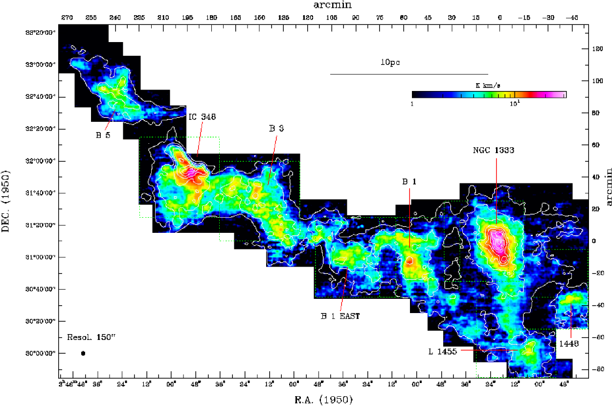
Figure 1: The Perseus molecular cloud complex. KOSMA maps of integrated intensities of ¹³CO 2–1 (colors) and ¹²CO 3–2 (contours) at $150^{\prime\prime}$ resolution. The integration interval is 0–16 km s^-1. Colors run from 1 Kkms^-1 ($\sim$ 1 $\sigma$) to 32 Kkms^-1. Contours range from 6.6 Kkms^-1 ($\sim$ 3 $\sigma$) to 83 Kkms^-1 in steps of 9 Kkms^-1. The (0,0) position corresponds to RA=03:26:00, DEC=$+31$:10:00 (B1950). Seven sub-regions are marked by dotted square boxes of $50^{\prime}\times 50^{\prime}$.

Figure 2 shows an overlay of integrated ¹³CO 2–1 intensities and a map of optical extinctions (Goodman, 2004; Alves et al., 2005), at $2.5^{\prime}$ and $5^{\prime}$ resolution, respectively. The ¹³CO map covers all regions above 7 mag and $\sim 70$% of the regions above 3 mag. A linear least squares fit to a plot of A_v vs. ¹³CO 2–1 results in a correlation coefficient of 0.76. The region mapped in ¹³CO has a mass of 1.7 $\times$ 10⁴ M_⊙ using the $A_{\mathrm{V}}$ data and the canonical conversion factor [H₂]/[$A_{\mathrm{V}}$] = 9.36 $\times$ 10²⁰ cm^-2 mag^-1 (Bohlin et al., 1978).

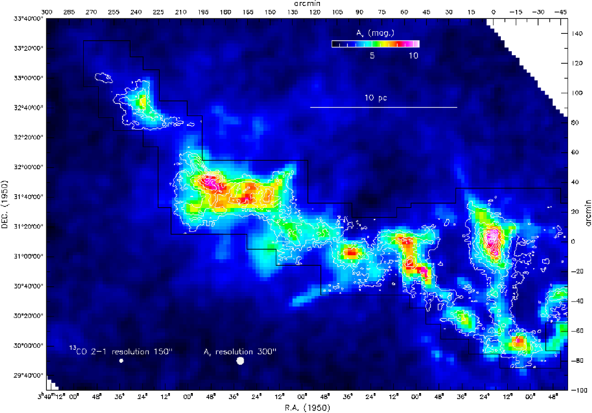
Figure 2: Overlay of ¹³CO 2–1 integrated intensities (contours) with a map of optical extinctions in colors (Goodman, 2004; Alves et al., 2005). Contours range from 2.7 Kkms^-1 (3 $\sigma$) to 32 Kkms^-1 by 3 Kkms^-1. Colors range from A_v = 1 mag to 11 mag. Resolutions are $2.5^{\prime}$ for ¹³CO and $5^{\prime}$ for $A_{\mathrm{V}}$. A polygon marks the boundary of the ¹³CO map.

3.2 Velocity structure

Maps of ¹³CO 2–1 emission integrated over small velocity intervals (Fig. 3) illustrate the filamentary structure of the Perseus clouds. The channel maps show the well-known velocity gradient between the western sources, e.g. NGC 1333 at $\sim$ 7 km s^-1, and the eastern sources, e.g. IC 348 at $\sim$ 9 km s^-1. The channel map integrated between 5 and 6 km s^-1 exhibits two filaments originating at L 1455, one runs north to NGC 1333, the second runs north-east to B 1. We will discuss the structural properties of individual velocity channel maps in the next sections.

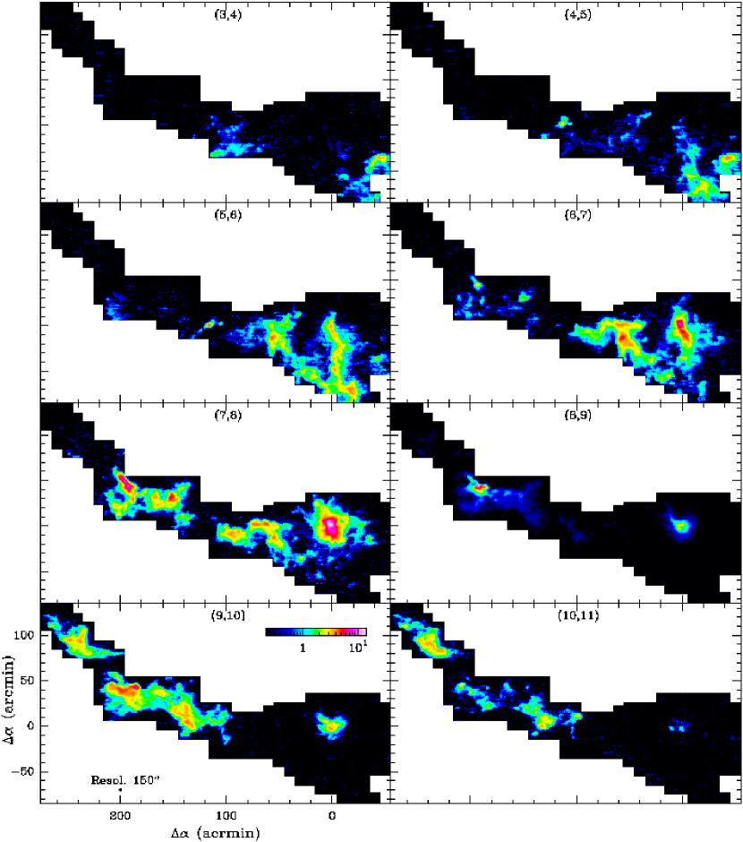
Figure 3: ¹³CO 2–1 velocity channel maps of the Perseus region. The velocity range runs from 3 km s^-1 to 11 km s^-1 with an interval of 1 km s^-1 which is indicated on the top of each plot. The intensities are plotted from 0.7 Kkm s^-1 ($\sim$ 1 $\sigma$) to 15 Kkm s^-1.

To study the statistics of the velocity field we start with the distribution of the line widths across the map. Since many spectra show deviations from a Gaussian line shape, we use the equivalent line width $\Delta v_{\rm eq}=\int Tdv/T_{\rm peak}$ as a measure of the line dispersion along individual lines of sight. Figure 4 shows the mean equivalent line widths and their scatter for the seven sub-regions shown in Figure 1.

The mean ¹²CO widths vary significantly between 2.2 km s^-1 in the quiescent dark cloud L 1455 and 3.8 km s^-1 in the active star forming region NGC 1333, while the rms is $\sim 0.7$ km s^-1. In contrast, the ¹³CO widths are smaller and show only a weak trend around $\sim 2$ kms^-1.

Several positions in L 1455, but also in e.g. IC 348, show small line widths of $\sim$1 km s^-1, only a factor of $\sim$8–11 larger than the CO thermal line width, which is $\approx$ 0.16 km s^-1 for a kinetic temperature of 10 K as was found for the bulk of the gas in Perseus by Bachiller & Cernicharo (1986).

Figure 4: Mean and rms of the equivalent line widths $\Delta v_{\rm eq}$ of the ¹²CO 3–2 and ¹³CO 2–1 spectra for the observed positions of the seven $50^{\prime}\times 50^{\prime}$ sub regions (Fig. 1). The dashed line delineates equal widths in ¹²CO and ¹³CO.

4 Structure analysis

In this section, we statistically quantify the spatial structure observed in the maps, both for the overall structure and for the structure of individual regions within the Perseus molecular cloud. We measure the spectral index of the power spectrum using the $\Delta$-variance analysis, a wavelet convolution technique. We analyze our new CO data and compare the results with an equivalent analysis of the FCRAO ¹²CO 1–0, ¹³CO 1–0 maps and the $A_{\mathrm{V}}$ Perseus map obtained from 2MASS (Two Micron All Sky Survey) by the COMPLETE team (Goodman, 2004; Alves et al., 2005).

4.1 The $\Delta$-variance analysis

The $\Delta$-variance analysis was introduced by Stutzki et al. (1998) as a means to quantify the relative amount of structural variation at a particular scale in a two-dimensional map or a three-dimensional data set. The $\Delta$-variance is defined as the variance of an image $s(\@vec{r})$ convolved with a normalized spherically symmetric wavelet $\odot$ of size $L$

$$\sigma^{2}_{\mathrm{\Delta}}=\langle\left[s(\@vec{r})\ast\odot_{\mathrm{L}}(\@vec{r})\right]^{2}\rangle_{\@vec{r}},$$ (1)

where the asterix denotes the spatial convolution (Stutzki et al., 1998). For structures characterized by a power-law spectrum, $P(|\@vec{k}|)\propto|\@vec{k}|^{-\beta}$, the $\Delta$-variance follows as well a power law, with the exponent $d_{\mathrm{\Delta}}=\beta-2$ in the range $0\leq\beta\leq 6$.

Unfortunately, the $\Delta$-variance spectrum of any observed data set does not only reflect the spectral index $\beta$ of the astrophysical structure, but it is also affected by radiometric noise and the finite telescope beam (Bensch et al., 2001). Both effects change the spectrum at small scales. When we ignore the small contribution from beam blurring, we can write the $\Delta$-variance as

$$\sigma_{\mathrm{\Delta}}^{2}(L)\approx a_{1}L^{\mathrm{\beta-2}}+a_{2}L^{\mathrm{d_{\mathrm{noise}}}},$$ (2)

(Eq. (10) from Bensch et al., 2001). For white noise, $\beta_{\mathrm{noise}}=0$, so that $d_{\mathrm{noise}}=-2$. In the KOSMA data we noticed that the noise does not follow a pure white noise behaviour, but it is “colored” due to artifacts from instrumental drifts, baseline ripples, OTF stripes etc. This has to be taken into account when deriving the cloud spectral index $\beta$ from the $\Delta$-variance spectra.

Thus we measured the spectral index of the colored noise $d_{\mathrm{noise}}$ by analyzing maps created from velocity channels which do not see any line emission but which cover the same velocity width as the actual molecular line maps. The result is shown in Fig. 5. We find a nearly constant index $d_{\mathrm{noise}}\approx-1.5$ for all off-line channels at scales between about 1 and 6′. At larger lags, the noise deviates from the $\beta$ = 0.5 behaviour, but this does not affect the structure analysis as the absolute noise contribution is negligible there.

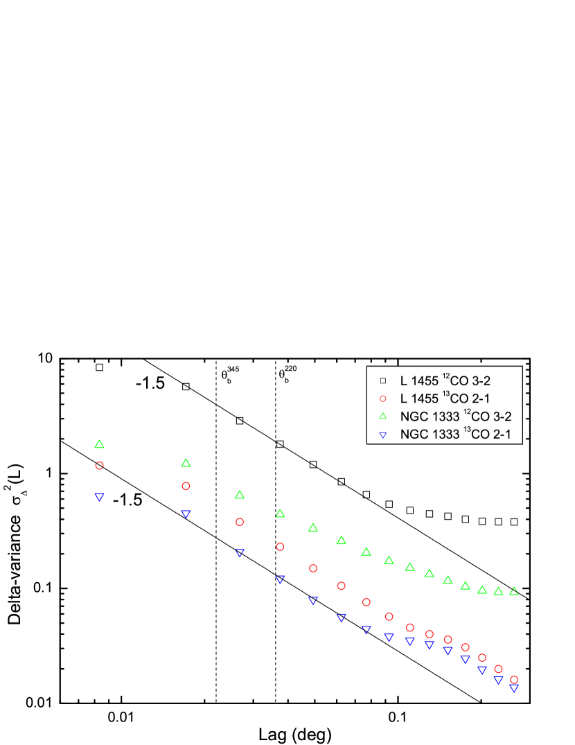
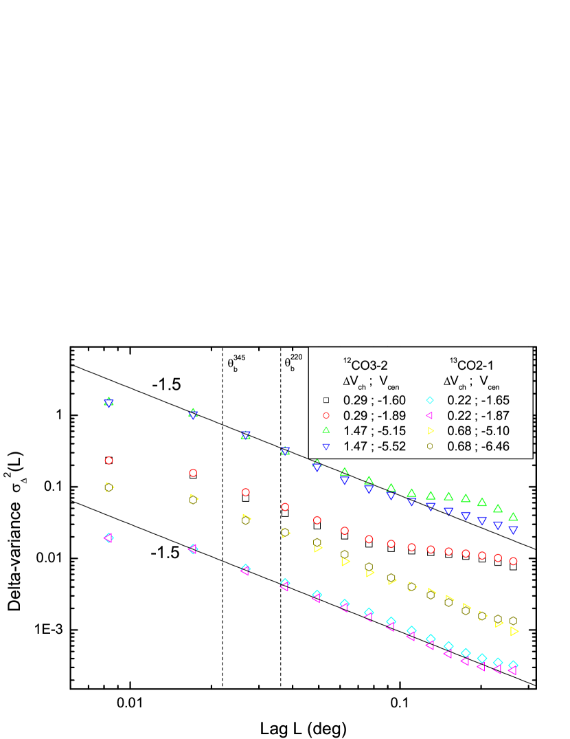
Figure 5: $\Delta$-variance analysis of the off-line channel maps. In the upper plot a velocity span corresponding to the integrated intensity maps is used. The two regions representing opposite extremes in the structural behaviour, NGC 1333 and L1455, show about the same spectral index of the colored noise in both transitions for small lags. In the lower plot, the influence of different velocity spans, as used in the velocity channel analysis (Sect. 4.3), is studied for L1455. The colored noise index $d_{\mathrm{noise}}$ is nearly constant independent of species, transition, velocity range $\Delta$v_ch, and center velocity v_cen.

For the FCRAO data and the COMPLETE $A_{\mathrm{V}}$ map we have no emission-free channels available so that we cannot perform an equivalent noise fit there. The $\Delta$-variance at small lags shows however no indications for a deviation from the pure white noise behaviour, so that we stick to $d_{\mathrm{noise}}=-2$ for the fit of these data.

4.2 Integrated intensity maps

Figure 6 compares the $\Delta$-variance spectra of the different integrated intensity maps for the entire region mapped with KOSMA (see Fig. 1). When corrected for the observational noise, the $\Delta$-variance spectra of all maps follow power laws between the linear resolution of the surveys and about 3 pc (Table 1). The good agreement of the spectral indices obtained from the different CO data is remarkable. They cover only the narrow range between 3.03$\pm$0.14 and 3.15$\pm$0.04. In contrast, the extinction data result in a significantly lower index. This indicates a more filamentary structure in $A_{\mathrm{V}}$. When we actually compare the $A_{\mathrm{V}}$ map with ¹³CO 2–1 data smoothed to the same resolution, it is also noticeable by eye that the $A_{\mathrm{V}}$ map looks more clumpy or filamentary than the ¹³CO map. This indicates that ¹³CO does not trace all details of the cloud structure, but rather measures the more extended, and thus more smoothly distributed gas.

All $\Delta$-variance spectra show a turnover at about 3 pc. To test whether this peak measures the real width of the Perseus cloud or whether it is produced by the elongated shape of the CO maps, we have repeated the $\Delta$-variance analysis for the $A_{\mathrm{V}}$ data of the entire region shown in Figure 2. In this case we find almost the same spectrum below 3 pc, but instead of a turnover only a slight decrease of the slope at larger lags. Thus we have to conclude that the $\Delta$-variance spectra of the CO maps at scales beyond 3 pc are dominated by edge effects, due to the shape of the maps, so that these scales should be excluded from the analysis. In Figure 6 we compare only spectra for the same region, i.e. the $\Delta$-variance spectra of the $A_{\mathrm{V}}$ data of the region also mapped with KOSMA.

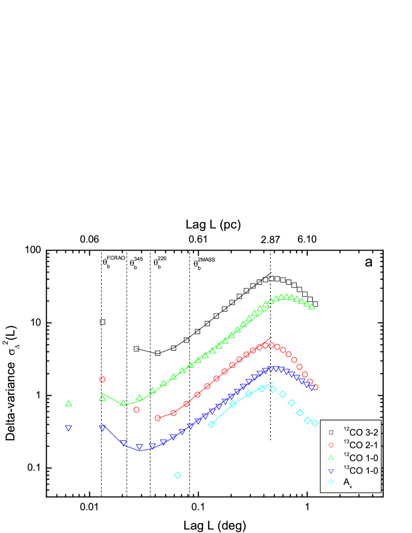
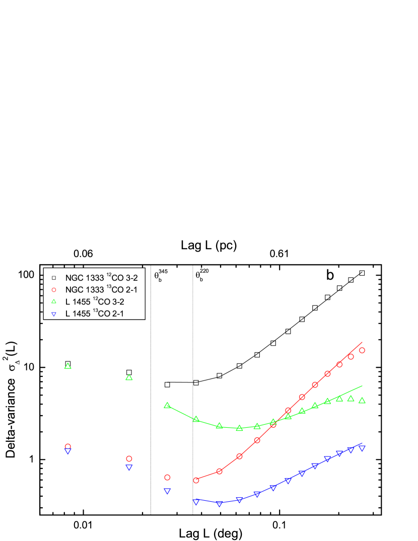
Figure 6: $\Delta$-variance spectra of integrated intensities. a) Spectra obtained from the CO maps and the $A_{\mathrm{V}}$ data of the region mapped with the KOSMA telescope. b) Spectra of integrated intensity maps of two 50′$\times$ 50′sub-regions: NGC 1333 and L 1455. Power-law fits to the data corrected for noise and beam-blurring are indicated as solid lines.

As it is not guaranteed that the structure of the overall region is representative for individual components, we have also applied the $\Delta$-variance analysis to the KOSMA data of the individual clouds contained in the seven $50\arcmin\times 50\arcmin$ subregions shown in Fig. 1. The results of the power-law fits to the $\Delta$-variance spectra are listed in Table 2. They differ significantly between the individual regions. The active star-forming region NGC 1333 shows the highest spectral indices in both transitions. The low end of the spectral index range is formed by the dark cloud L 1455 together with the environment of the young cluster IC 348. The $\Delta$-variance spectra of the two extreme examples NGC 1333 and L 1455 are shown in Fig. 6b. Starting from the same noise values at small scales the spectra of the two regions show an increasing difference in the relative amount of structure at large scales reflected by the strongly deviating spectral indices. Altogether, we find high indices as characteristics of large condensations for the regions with active star formation and lower indices quantifying more filamentary structure for dark clouds, but IC 348 as an exception to this rule, showing also a very filamentary structure.

Table 1: Results of the $\Delta$-variance analysis of the integrated CO maps and the $A_{\mathrm{V}}$ data for the region mapped with KOSMA (Fig. 1).

Transition	Telescope	resol.	Fit Range	$\beta$
		[′]	[′]
$A_{\mathrm{V}}$	2MASS	5	5.0-28	2.55 $\pm$ 0.02
13CO 1–0	FCRAO	0.77	0.8-28	3.09 $\pm$ 0.09
12CO 1–0	FCRAO	0.77	0.8-28	3.08 $\pm$ 0.04
13CO 2–1	KOSMA	2.17	2.2-28	3.03 $\pm$ 0.14
12CO 3–2	KOSMA	1.37	1.4-28	3.15 $\pm$ 0.04

Table 2: Results of the $\Delta$-variance analysis of the KOSMA data for seven 50′$\times$ 50′sub-regions of the cloud (Figure 1). The spectral indices $\beta$ were fitted in the size range 2.2-14^′ for the ¹³CO 2–1 and in the size range 1.4-14^′ for the ¹²CO 3–2 data.

Region	$\beta(^{13}$CO$\,2-1)$	$\beta(^{12}$CO$\,3-2)$
L 1448	2.96 $\pm$ 0.42	3.41 $\pm$ 0.16
L 1455	2.86 $\pm$ 0.09	2.85 $\pm$ 0.30
NGC 1333	3.76 $\pm$ 0.48	3.52 $\pm$ 0.11
B 1	3.14 $\pm$ 0.29	3.00 $\pm$ 0.20
B 1 EAST	3.16 $\pm$ 0.09	3.39 $\pm$ 0.09
B 3	3.36 $\pm$ 0.09	3.14 $\pm$ 0.06
IC 348	2.71 $\pm$ 0.42	3.06 $\pm$ 0.24

4.3 Velocity channel maps

When performing the $\Delta$-variance analysis not only for maps of integrated intensities, but for individual channel maps we obtain additional information on the velocity structure of the cloud. In the velocity channel analysis (VCA), introduced by Lazarian & Pogosyan (2000), the change of the spectral index of channel maps as a function of the channel width was used to simultaneously determine the scaling behavior of the density and the velocity fields from a single data cube of line data. Here we conduct such a study for the KOSMA CO data.

We start with the analysis of individual channel maps as they are provided by the channel spacing $\Delta$v_ch of the backends (cf. §2). For all channel maps we perform the $\Delta$-variance analysis and fit power laws to the measured structure for all lags between the telescope beam size and the maximum scale resolved by the $\Delta$-variance (about 1/4 of the map size). As a result we get the power-law index as a function of the channel velocity, a curve which we call index spectrum. As an example we show the index spectrum obtained for the ¹³CO 2–1 data in the L 1455 region in Fig. 7. The spectrum is always truncated at velocities where the average line temperature is lower than the noise rms.

The overall structure of the index spectrum is similar to the line profile. The largest spectral indices are found at velocities close to the average line peak. This may implicate that extended smooth structure provides the major contribution to the overall emission, while the velocity tail of this structure is formed by small-scale features. However, the indices show an asymmetric behavior with respect to the blue and the red wing. The indices drop steeply to a noise-dominated value at the red wing, while the blue wing shows only a very shallow decay. Even at the noise limit, noticeable structure is detected in the channel maps there.

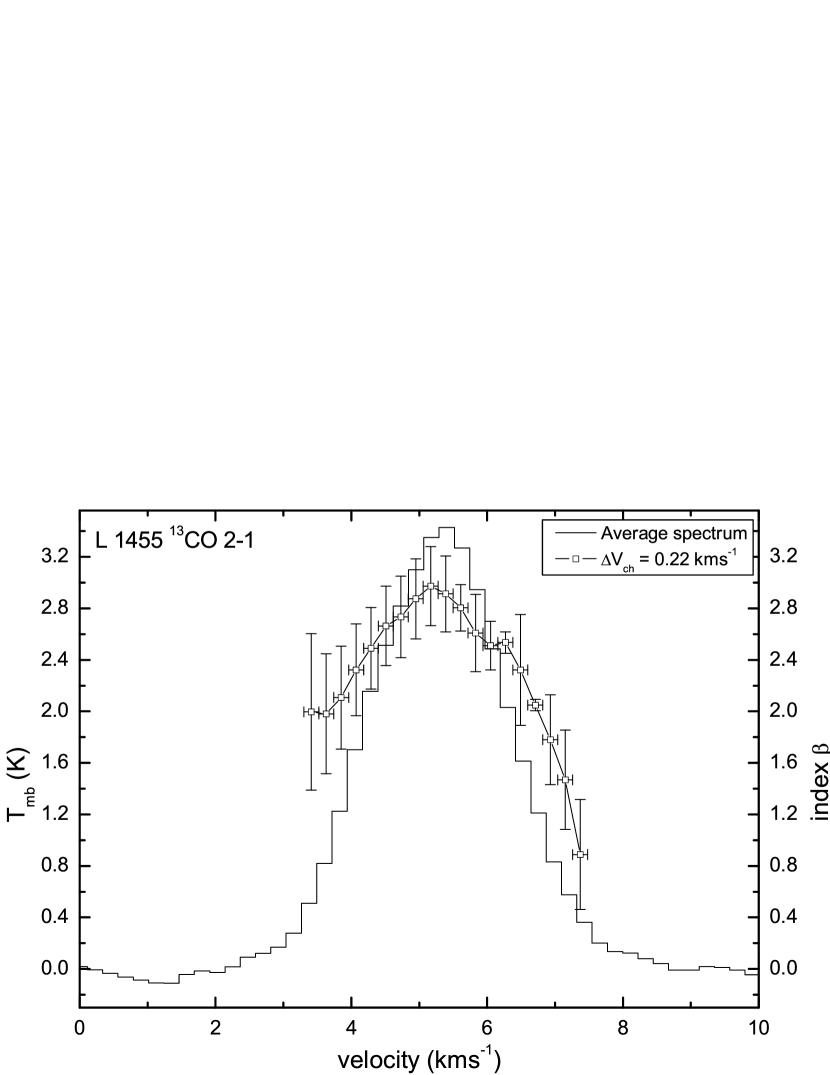
Figure 7: Comparison of the index spectrum of the ¹³CO 2–1 data in L 1455 with the average line profile. The index spectrum is created by power-law fits to the $\Delta$-variance spectrum of individual channel maps ($\Delta$v_ch = 0.22 km s^-1). The vertical error bars represent the uncertainty of the fit. The horizontal error bars indicate the velocity channel width.

For the full velocity channel analysis, the index spectrum has to be computed for different velocity channel widths (Lazarian & Pogosyan, 2000). Thus we have binned the data to averages of three, five, and seven velocity channels and computed the index spectra for these binned channel maps. In Fig. 8 we show the results for three examples: IC 348, NGC 1333 and L 1455. For the sake of clarity the error bars of the index spectra were omitted in these plots.

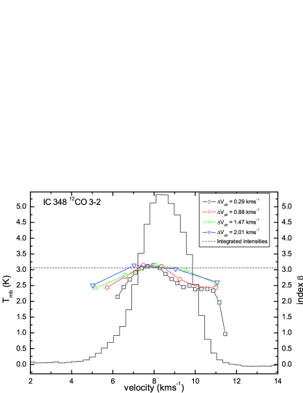
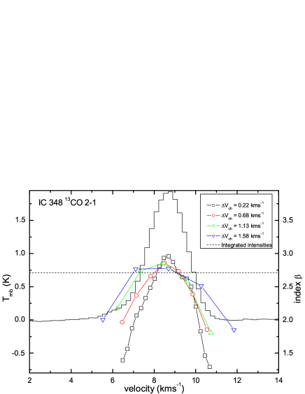
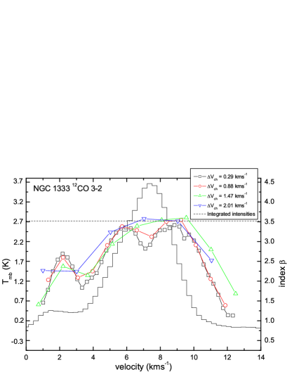
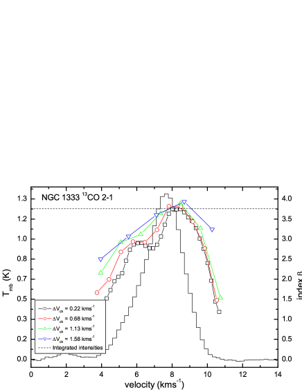
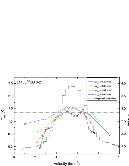
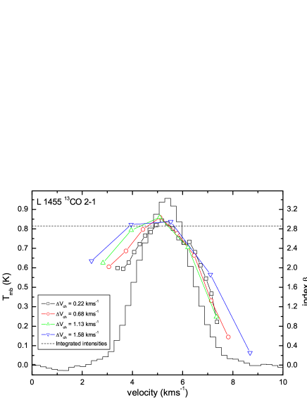
Figure 8: Comparison of the index spectra obtained for different velocity channel widths with the average line profile. The upper plots show the results for IC 348, the central plot NGC 1333 and the lower plot L 1455. For the left column we used the ¹²CO 3–2 data, the right column represents the ¹³CO 2–1 data. The different symbols indicate the results from different velocity channel widths. The dashed lines represents the index of the integrated intensity maps.

The overall structure of the index spectra is similar to Fig. 7 for all sources, transitions and channel widths. In most cases we find the asymmetry of a shallower blue wing relative to the red wing. When looking at narrow velocity channels, we find a dip in the centre of the index spectrum for the ¹²CO 3–2 data of NGC 1333 and L 1455. A slight indication of such a dip is also present in the ¹²CO 3–2 data if IC348 and in the ¹³CO 2–1 data of NGC 1333. This is due to optical depth effects. When we check individual spectra in those regions, we see self-absorption in several positions. This leads to a more filamentary appearance of the central channel maps reflected by this dip in the index spectra. It is interesting to notice that the VCA is more sensitive to self-absorption than the average spectrum.

When increasing the channel width by binning, the self-absorption dip is smoothed out, so that the resulting index spectra peak again close to the peak velocity of the line temperature. In all situations where the self absorption is negligible, the indices for the line core channels are almost independent from the channel width. The indices for the line integrated intensities always fall slightly below the peak indices, as they represent an average which is typically dominated by the line cores.

In the red line wings, most indices remain approximately constant when increasing the velocity width, except for the largest bin width where the contribution from the core leads to an observable increase. In the blue wing, we find a monotonic growth of the spectral indices with the channel width for both tracers in all three regions. The additional peak at 2 km s^-1 visible in the ¹²CO 3–2 data of NGC 1333 stems from a separate dark cloud which is also contained in the NGC 1333 map.

Figure 9 summarizes the relation between the spectral indices and the velocity channel width. In Fig. 9a we plot the average spectral index over the line as a function of the channel width for the six data sets presented in Fig. 8. Figure  9b contains the analysis when restricted to a 2 km s^-1 window in the blue line wings. The error bars contain the standard deviation of the index variation across the line and the fit errors. They are necessarily large because of the systematic variation of indices over the velocity range. In contrast to similar analysis by Dickey et al. (2001); Stanimirović & Lazarian (2001) we find no significant systematic variation of the mean line index as a function of channel width (Figure 9a). In contrast to the average of the index spectrum we find a continuous increase of the spectral index with the channel width when restricting the analysis to the blue wing (Figure 9b). The average index steepens from about 2.8 to about 3.1 in the ¹²CO 3–2 maps and from about 2.4 to about 2.8 in the ¹³CO 2–1 maps. As discussed above we find no systematic trend in the red wings. This indicates that the average spectral index taken over the full line profile provides no measure for the velocity structure in our CO maps while the peculiar behaviour in the blue wings needs further investigation.

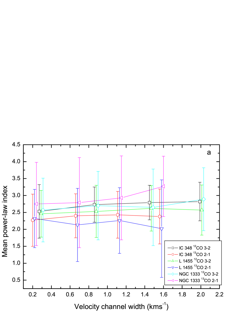
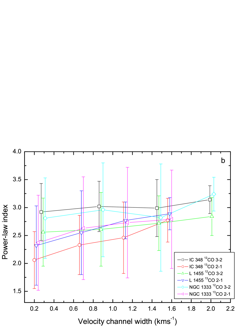
Figure 9: Average spectral indices of the channel maps as a function of the channel width. a) shows the average over the full line width. b) represents only the indices in the blue ling wings. The line wing components are centered at 5 km s^-1 for NGC 1333, at 4 km s^-1 for L 1455, and at 7 km s^-1 for IC 348. The error bars contain the fit error and the standard deviation of the indices within the considered velocity range. To avoid overlapping error bars in the plot, we have shifted the points for IC 348 and NGC 1333 by $\pm 0.02$ km s^-1 relative to their actual position.

5 Discussion

5.1 Integrated intensity maps

Besides the $\Delta$-variance, other tools have been used to characterize interstellar cloud structure. The second-order structure function for an observable $s(\@vec{r})$ is $S_{\mathrm{2}}=\langle|s(\@vec{r})-s(\@vec{r}+\delta\@vec{r})|^{2}\rangle_{\@vec{r}}$ which is treated as a function of the absolute value of the increment $|\delta\@vec{r}|$ (Elmegreen & Scalo, 2004). Padoan et al. (2003a) computed the structure function of the integrated intensity map of ¹³CO 1–0 in Perseus. A power-law fit to S₂ $\propto$ $\delta$r^ζ over a range of 0.3 to 3 pc provided an index $\zeta$ of 0.83. The index of the structure function is related to the power spectral index by $\zeta=\beta-2$ for $2<\beta<4$ (Stutzki et al., 1998) resulting in $\beta=2.83$. This result of Padoan et al. (2003a) agrees within the error bars with the indices found by the $\Delta$-variance analysis of the Perseus maps of integrated CO intensities over almost the same linear range (see Table 1).

However, the $\Delta$-variance spectra of individual regions show significant variations of the spectral index as discussed above. For ¹³CO 2–1, these span the range between $\beta=2.86$ in L1455 and 3.76 in NGC 1333 (Table 2). The analysis of different sub-sets in molecular cloud complexes thus provides additional and complementary information on the structure of the cloud complex.

5.2 Velocity channel maps

The velocity channel analysis (VCA), was used previously by Dickey et al. (2001) to study H i maps of two regions in the 4th Galactic quadrant. One of the regions is rich in warm H i gas, the other is rich in cool H i gas. For the warm gas, Dickey et al. (2001) find a systematic increase of the mean index with velocity channel width. The cold gas at lower latitudes behaves differently and shows rather constant indices of 2.7–3.1.

The latter results resemble the outcome of the VCA of the ¹²CO and ¹³CO channel maps in Perseus presented above. We find similar indices for the velocity integrated maps of the full region (cf. Table 1) and the CO data show no significant variation of the index with velocity channel width when averaged over all velocity bins (Figure 9a). The indices stay relatively constant. Since the bulk of the molecular gas traced by CO is even colder than cold H i gas, these results suggest a sequence of a reduced dependence of the spectral index of the channel maps on the bin widths from the warm to the cold ISM. The constancy of the average spectral index could also be explained by optical depth effects. Lazarian & Pogosyan (2004) have shown that absorption can lead to an effective slice broadening, which leads in extreme cases to slice indices that become independent from the actual channel width.

Studying the spectral index of individual velocity bins of the CO data across the line profile (Fig. 8), we find that the power-law indices increase with the velocity channel width in the blue wing (Fig. 9b) while staying rather constant in the red wing. No corresponding analysis was conducted for the H i data by Dickey et al. (2001). One possibility to explain the asymmetry between the blue and red wings might be a shock expansion of the CO gas in Perseus. Sancisi (1974) found an expanding shell of neutral hydrogen which was created by a supernova in the Per OB2 association a few $10^{6}$ years ago. At the location of the molecular cloud complex, the expansion is directed away from the Sun. Most of the associated molecular gas has been swept up by the shock, but pillar-like filaments have been left at the backside of the shock. They are visible in the channel maps (Fig. 3) and produce the velocity dependence seen in the VCA of the blue line wings, i.e. the increase of indices with size of the velocity bin because of a gradual increase of large scale contributions across the line wing. We illustrate this scenario in Fig. 10.

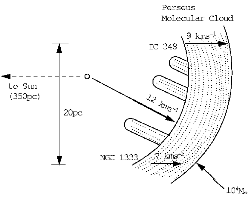
Figure 10: Sketch adopted from Fig. 3 of Sancisi (1974) illustrating the spatial arrangement and motion of the Perseus cloud complex. The gas is swept up by a shock expansion with 12 km s^-1. Due to the overall curvature, the line-of-sight velocity is 9 km s^-1 for IC 348, but only 7 km s^-1 for NGC1333. The diameter of the cloud is $\sim$ 20 pc. Pillar-like structures are left at lower velocities as remainders of high-density regions which were not accelerated to the same velocity.

The quantitative results from the velocity channel analysis can be interpreted in terms of the power spectrum of the velocity structure. Lazarian & Pogosyan (2000) showed that the spectrum of velocity slices as a function of the velocity channel width is determined by the power spectral indices of the density structure $\beta$ and the velocity structure $m$. They obtain different regimes for shallow ($\beta<3$) and steep ($\beta>3$) density power spectra:

$P(k)\propto\left\{\begin{array}[]{ll}k^{\mathrm{-\beta+\frac{m-3}{2}}},&\hbox{thin slices,}\\ k^{\mathrm{-\beta}},&\hbox{thick slices,}\\ k^{\mathrm{-\beta}},&\hbox{very thick slices;}\\ \end{array}\right.(\beta<3)$

$P(k)\propto\left\{\begin{array}[]{ll}k^{\mathrm{-\frac{9-m}{2}}},&\hbox{thin slices,}\\ k^{\mathrm{-\frac{3+m}{2}}},&\hbox{thick slices,}\\ k^{\mathrm{-\beta}},&\hbox{very thick slices.}\\ \end{array}\right.(\beta>3)$

Thin slices have a velocity width less than the local velocity dispersion at the studied scale; thick slices have a width larger than the velocity dispersion and very thick slices essentially correspond to the integrated maps (Lazarian & Pogosyan, 2000). We can assume that a single channel of our data corresponds to thin slices as they are much narrower than any observed line width. We use $\beta$ from the integrated maps and the index measured in the single channels to derive $m$. From the indices obtained by averaging over the full line profile (Fig. 9a), we obtain $m$ values of 3.9$\pm$1.6, 3.9$\pm$1.9 and 3.8$\pm$1.7 for ¹²CO 3–2 in IC 348, NGC 1333 and L 1455, respectively; while $m$ is 3.9$\pm$2.0, 3.5$\pm$2.5 and 4.1$\pm$1.8 for ¹³CO 2–1 in the same three regions. In the blue wings (Fig. 9b), we obtain $m$ values of 3.2$\pm$1.6, 3.4$\pm$1.4 and 3.6$\pm$1.5 for ¹²CO 3–2; while $m$ is 4.3$\pm$1.9, 4.3$\pm$1.7 and 4.1$\pm$1.5 for ¹³CO 2–1 in the three regions. These values have large error bars, so that they are not directly suited to discriminate between different turbulence models. At least, we find that all values are consistent with Kolmogorov turbulence that gives $m\sim 3.7$ (Kolmogorov, 1941).

6 Summary

1. We present KOSMA maps of the ¹³CO 2–1 and ¹²CO 3–2 emission of the Perseus molecular cloud covering 7.1 deg². These data are combined with FCRAO maps of integrated ¹²CO and ¹³CO 1–0 intensities and with a 2MASS map of optical extinctions.

2. To characterize the cloud density structure, we applied the $\Delta$-variance analysis to integrated intensity maps. The $\Delta$-variance spectra of the overall region follow a power law with an index of $\beta=2.9-3.0$ for scales between 0.2 and 3 pc. This agrees with results obtained by Padoan et al. (2003a) studying structure functions of a ¹³CO 1–0 map of Perseus.

3. We also applied the $\Delta$-variance method to seven sub-regions of Perseus. The resulting power spectral indices vary significantly between the individual regions. The active star-forming region NGC 1333 shows high spectral indices ($\beta=3.5-3.8$) while the dark cloud L 1455 shows low indices of 2.9 in both transitions.

4. Additional information is obtained from the $\Delta$-variance spectra of individual velocity channel maps. They are very sensitive to optical depth effects, indicating self-absorption in the densest regions. The asymmetry of the channel map indices relative to the line centrum is a hint towards a peculiar velocity structure of the Perseus cloud complex.

5. When analyzing the spectral indices as a function of the velocity channel width we find almost constant indices when averaging over the total line profile. A continuous increase of the index with varying velocity channel width is, however, observed in the blue wings. This behavior can be explained by a shock running through the region creating a filamentary structure preferentially at low velocities.

We find that the comparison of the structural properties for entire surveys and sub-sets, as well as the velocity channel analysis (VCA), provide additional, significant characteristics of the ISM in observed CO spectral line maps. These quantities are useful for a comparison of the structure observed in different clouds, possibly providing a diagnostic tool to characterize the star-formation activity and providing additional constraints for numerical simulations of the ISM structure.