Far-ultraviolet Observations of the North Ecliptic Pole with SPEAR
Abstract
We present SPEAR/FIMS far-ultraviolet observations near the North Ecliptic Pole. This area, at 30∘ and with intermediate Hi column, seems to be a fairly typical line of sight that is representative of general processes in the diffuse ISM. We detect a surprising number of emission lines of many elements at various ionization states representing gas phases from the warm neutral medium (WNM) to the hot ionized medium (HIM). We also detect fluorescence bands of , which may be due to the ubiquitous diffuse previously observed in absorption.
Subject headings:
ISM: general, ISM: lines and bands, ultraviolet: ISM1. Introduction
The North Ecliptic Pole (NEP) is a region of the sky with no obviously unusual features. Many prior space-missions (Einstein, ROSAT, COBE, IRAS, etc.) have conducted deep surveys of this region. Several ground based surveys have also concentrated on this region as a complement to the space-based surveys (Labov et al., 1989; Elvis et al., 1994). Its location at moderate galactic latitude (b=+29∘) places it clear of the bright stars of the galactic plane. In this region, the Galactic N(HI) varies from about 2 to 8 which corresponds to an dust opacity of =0.6-2.3 at 1032Å(Sasseen et al., 2002) or =0.3-1.4 at 1550Å(Savage & Mathis, 1979).
The Spectroscopy of Plasma Evolution from Astrophysical Radiation (SPEAR) instrument, designed for observing emission lines from the diffuse ISM was launched in late 2003. SPEAR is a dual-channel FUV imaging spectrograph (short- (S) channel 900 - 1150 Å, long- (L) channel 1350 - 1750 Å) with 550, with a large field of view (S: 4.0 4.6’, L: 7.5 4.3’) imaged at 10 resolution. See Edelstein et al. (2005a, b) for an overview of the instrument, mission, and data analyses. SPEAR sky-survey observations consist of sweeps at constant ecliptic longitude from the NEP to the south ecliptic pole through the anti-solar point. The duration of each sweep varies between 900 and 1500 s. Each survey scan includes the region near the north and south ecliptic poles resulting in large exposure times in these regions. We report on deep SPEAR observations of FUV emission spectra from a 15∘ radius region centered on the NEP.
2. Observations and Data Reduction
The NEP data analyzed here include sky-survey and pointed observations that occurred between 8 November 2003 to 10 November 2004. To remove times of high background and bright stars from the data set, we have excluded times during which the count rate exceeds 100 s-1. (In comparison, a typical photon count rate is s-1.) Because stars transit the instrument slit in s during survey sweeps, this results in minimal loss of observing time. The area of sky lost due to a star is similar to the instrument imaging resolution across the slit width (). See Edelstein et al. (2005a) for a description of the data reduction pipeline.
To further remove stellar contamination from our dataset, we excluded locally intense spatial bins (30% of the viewed area), defined to have the median count rate. This level corresponds with a slope change in the histogram of the log count rate, indicative of a difference in distribution of scattered vs direct starlight. Inclusion of unresolved starlight should not be a factor other than to raise emission-line determination errors. To obtain the highest sensitivity possible, we have binned the entire dataset into a single spectrum including a total of 3.5 counts over an effective full-slit exposure of 13.5 ks.
3. Spectral Modeling
The raw SPEAR spectrum is composed of many components: detector background, dust-scattered stellar continua, direct and instrumentally scattered airglow, and IS atomic and molecular emission. To model a spectrum we simultaneously fit all of the components to the observed spectrum.
The spectral shape is distorted by the detector electronics and by the data processing pipeline. These distortions appear as fluctuations in a flat-field image. Any broad-band component used in our model spectrum must be multiplied by this nonlinearity function. (Korpela et al., 2003; Rhee et al., 2002).
Both S and L are affected by instrumental background due to cosmic rays, radioactive decay within the detector, and thermal charged particles entering the instrument. These sources of background are relatively uniform across the face of the detectors. Although the charged particle rate can change with time and orbital position, the positional distribution of these background events is dominated by static fields within the instrument and is relatively constant. A sum of many shutter-closed dark exposures multiplied by a rate factor can be used to model this contribution to the spectrum.
In L, the largest broad-band spectral component is dust scattered stellar continua. We model the input spectrum to the dust scattering process as a sum of spectra for upper main sequence (UMS) stars. Each spectrum is weighted by using a power law UMS luminosity function (, where is the absolute magnitude and is the volume density of stars per unit magnitude) and a dilution factor dependent upon the weighted mean distance of the stars. The spectral sum is multiplied by a dust opacity scaled to a variable and by a dust albedo function (Draine, 2003) with a variable total dust surface area. The best fits for this function typically occur very near to the measured UMS luminosity function with (Reed, 2001). Because the stellar features in this spectrum cannot be directly measured, there may be some bias in our measurements of the overlying resonance lines (Civ 1548,1551, Ovi 1032,1038, Siiv 1394,1403, etc.) of order (LU). We include this effect in our error analysis. Our best fit continuum, which could include unresolved stars, is (CU) in L. In S, due to its lower sensitivity and higher non-astrophysical background, we are only able to place a statistical upper limit of CU. However, given the wavelength dependence of the dust albedo, we expect that the true S astrophysical continuum is no higher than in L.
We first attempted to fit atomic line emission by using linear combinations of collisional ionization equilibrium (CIE) plasma models with a limited abundance gradient vs . We attribute this method’s lack of success to photoexcitation of resonance lines, non-CIE effects and abundance variations that are not related. To fit the line emission we have, instead, fit the spectrum of each species separately with a per-species intensity and parameter. The emission line spectra are convolved with a -dependent Gaussian to model the instrument spectral resolution. We use the atomic parameters of CHIANTI (Young et al., 2003) to determine the spectrum of the species vs . This spectrum is then normalized and multiplied by the intensity parameter. When CHIANTI parameters are not available for a species, we use a spectrum calculated using the NIST Atomic Spectra Database.
We then consider the effects of self-absorption of spectral resonance lines. In the case of highly ionized species we assume all lines are optically thin. We also assume this to be the case for species that would be completely photoionized in the WNM (ionization potential (IP) ). For species which are likely to be abundant in the WNM and warm ionized medium (WIM), (IP ) we assume that resonance lines are optically thick () and that the distances to the illuminating stars are large compared to the surface. In cases where the ground state is split, absorbed resonance line photons will be converted to the excited state, greatly changing the relative contributions in the multiplet. We model this by attenuating the ground state transition by a large factor. We will develop a more accurate way of treating these optical depth effects in future work.
4. Discussion
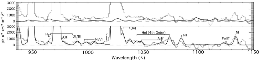
The spectrum of the bright Lyman-series geocoronal emission, easily visible in Fig. 1, can be modeled using a temperature and total line flux. The largest S broadband component is scattered geocoronal 1216 emission. This line occurs in the bandpass gap between S and L. L is immune to contamination because it includes a filter which is very nearly opaque to radiation. We fit the S scattering with two components, an exponential scatter with Å, and an isotropic component. The scattering, summed over the entire spectrum, is 0.08% of a 5 kRy incident flux. Because the transition is optically thick, and because the scattering fractions are independent parameters, we fix the estimated incident flux at 1100 the flux which helps the solution to converge. While the fractional scatter and exponential width of these components are free parameters in our spectral model, the values we obtain vary little from one dataset to the next.
Our model includes spectral features of atmospheric Oi, Ci, and Ni that are much fainter than when seen in day-time observations (e.g. FUSE), as SPEAR only observes during orbital eclipse. We detect a spectral feature near 990 Å that is consistent with the Oi 989 transition. However, this feature may be blended with Niii 990. If the entirety of the 990 Å feature is due to Oi, the lack of detectable Oi 1356 emission would indicate K, which is plausible for interstellar Oi. We do detect Oi 1356 in data that is not count rate filtered. The other possibility is that the 990 Å is due to Oi at few hundred K which seems unlikely even for atmospheric Oi. The most likely explanation for the lack of any detection of Oi emission at is that a large portion, if not all, of the 990 Å emission is due to Niii.
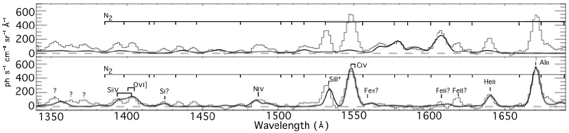
We detect relatively strong emission from fluorescence bands even in this region of intermediate . This is not entirely surprising since absorption due to is a ubiquitous feature of FUV spectra taken by FUSE. (Shull et al., 2000) We fit these features by using interpolation between of a sparse grid of models (B. Draine 2004, private communication). The upper panels of Figs. 1 & 2 show the best fit model plotted against the residuals of the spectrum following background, continuum, and scattering subtraction. We detect H2 emission features in both spectral bands. In S we detect the 965 band (to the left of the HI 972 line) and the 986 band (to the left of the Oi,Niii 989 feature). The 1053 and 1097 bands are not detected at any significance. In L, H2 provides contributions throughout the spectrum. We attribute the triple peaked band structure between 1350 and 1380 Å, the peak near 1440 Å, the broad features 1520-1530, 1570-1590, and the peak near 1608Å to H2. Note that these features are not well fit by our model. It is not surprising that our sparse linear model with a single dust absorption column does not fit these data since the observed emission derives from many lines of sight with varying illumination, gas temperatures and absorbing columns. In Figs. 1 & 2, lower panels we show the residual spectrum following subtraction of the H2 component.
We see intriguing indications of fluorescent emission , most notably the features at 1434Å, 1445Å, 1475Å, and 1660Å. FUSE has detected absorption due to along some sight-lines, albeit at shorter wavelengths (Knauth et al., 2004). We cannot yet discount the possibility that these features are atmospheric, as near the magnetic poles, can be transported to high altitude. Further study to determine whether the emission varies with spacecraft orbital position or with galactic latitude of the observation should resolve this question. If confirmed as astrophysical, this would be the first detection of fluorescent emission from the diffuse ISM.
SPEAR has discovered some surprising spectral features, such as the resonance lines of the singly ionized species, Siii and Alii. The Alii feature at 1671 Å very nearly overlies the Oiii] 1665 which we do not detect in this dataset. In a lower resolution instrument these spectral features could be blended resulting in confusion of the Oiii] and Alii emission. We think it is likely that at least some of the prior claimed detections (Martin & Bowyer, 1990) of Oiii] were in fact misidentified detections of Alii 1671. We attribute the feature at 1533 Å to the Siii∗ 1533.4 transition into the upper fine structure level of the ground state. The offset between the model feature and the observed line may be due to an uncorrected continuum feature underlying this line (Fig. 3 of Edelstein et al. (2005a)). Since Siii is the predominant state of silicon in both the WNM and WIM, the true Siii 1526.7 ground state transition is likely to be optically thick and therefore undetectable. Our spectral models are improved by the addition of Feii transitions throughout band, most notably the Feii 1564, which fills the gap between Civ 1548,1551 and the 1570-1590 H2 band. It is also possible that there is a contribution to the 1600-1620 band due to the Feii 1608 resonance lines. These lines have a fairly low oscillator strength and are expected to be optically thin along this line of sight. However, given the low oscillator strength, we expect these lines to be faint compared to the Siii and Alii features.
| Species | Statistical | Model | ||
|---|---|---|---|---|
| Error | Uncertainty | |||
| Å | LUa | LU | LU | |
| Oiii] | 1667 | b | – | – |
| Oiv] | 1400 | 1980 | 220 | 300 |
| Ovi | 1032,1038 | 5724 | 570 | 1100 |
| Ciii | 977 | 1260 | 270 | – |
| Civ | 1548,1551 | 5820 | 280 | |
| Siii∗ | 1532 | 2430 | 200 | |
| Siiv | 1394,1403 | 1430 | 120 | 160 |
| Nii | 1085 | 8500 | 730 | – |
| Niii | 990 | – | – | |
| Niv | 1485 | 1984 | 170 | 450 |
| Alii | 1671 | 5608 | 525 | – |
| Heii | 1640 | 1850 | 180 | |
| Nevi | 999,1005 | – | – |
Note. — aLU= bUpper limits are 90% confidence
Emission lines of highly ionized gas expected to be generated in a CIE plasma at HIM temperatures are shown in Table 1. Of these we detect () Ciii 977, Civ 1548,1551, Siiv 1394,1403 and Ovi 1032,1038. The Civ 1549 and Siiv 1400 emission overlie prominent stellar absorption features which are likely to be present in the dust-scattered stellar radiation. Since the depth of these features is unknown we set the lower range of our model uncertainty to be the intensity that would be calculated if there were no continuum feature present.
Many of these emission features are resonance lines (R. J. Reynolds 2005, private communication) and, because of the substantial IS radiation field at these wavelengths, further work will be required to determine whether these lines arise due to collisional excitation in the HIM or due to resonant scattering of the IS radiation field. We believe that the short wavelength lines are less likely to be resonant scatter because the relative intensity of the scattered stellar continuum in the S band is much lower (Korpela et al., 1998).
Our Civ 1548,1551 intensity of 5820280 LU is marginally higher than values for the diffuse ISM reported by Martin & Bowyer (1990). However Martin and Bowyer assumed a featureless continuum rather than a continuum with stellar features. If we make the same assumption our value drops to 4330210 LU which is more within the range of values they report.
Our Ovi 1032,1038 intensity of 57241100 LU is somewhat higher than the typical value measured by FUSE (Shelton, 2003). This could be a systematic effect due to the uncertain calibration of the S band. In fact the ratio of the feature intensities between L and S suggests that we have underestimated the sensitivity of S. Since this is an average over a very large region, it is also possible that the Ovi emission is due to several small regions with very high intensity, such as SNR.
The double peaked feature near 1400 Å is a blend of Siiv 1393.8,1402.8 and Oiv] 1400.7,1407.4. The Oiv] emission is of great interest because, as a semiforbidden line, it is not strongly affected by the radiation field, but is a direct indicator of collisional processes. Assuming a 2:1 ratio for the Siiv doublet components, our model determines the Oiv] doublet intensity to be 1980300 LU and the Siiv doublet intensity to be 1430160 LU.
We detect high stage ions of two noble gases in our spectra, Heii 1640 and Nevi 999,1005. Although the features corresponding to the Nevi lines are statistically significant, the poor fit to the underlying bands prevents us from placing more than an upper limit to these features. Because of the lack of detection of any Oi 1356, we do not expect any contamination of the Heii line with Oi 1641. The Heii line is much brighter than would be expected in a solar abundance CIE model (in ratio to Ciii and Oiii). This could be due to depletion of C and O to solar. A depletion of this magnitude would be significantly higher than the accepted values for the ISM.
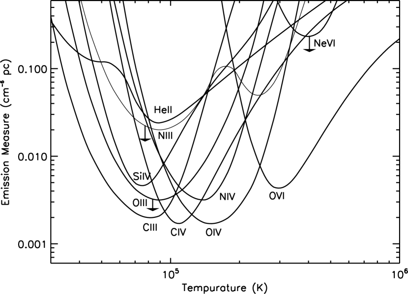
In Fig. 3 we show equivalent solar abundance emission measure (EM) and limits for several species. The results are not entirely consistent between species. For example higher EM is necessary to explain the Siiv and Heii emission than are compatible with the amount of Ciii emission. The questionable Nevi detections would indicate EM 10 that suggested by the Ovi measurements. The bulk of the inconsistency in Nevi is likely to be due to undersubtraction of the underlying H2. Much of the inconsistency in other lines is likely due to non-CIE effects which are present in gas being heated or cooling at these temperatures. Some portion of the difference could be due to abundance variations (with ISM depletions of O and C higher than those of Ne, He, and Si), although the suggested depletions are much higher than the accepted ISM values. In future work we will derive constraints to non-CIE cooling models and abundances using these line ratios.
5. Conclusions
We have presented the FUV spectra of a 30∘ region around the NEP. We detect a variety of emission lines from high and low ionization gas. The high ionization lines, taken on a per species basis, are consistent with EM from 0.001 to 0.005 throughout to 105.5 K range. For those few species which have multiple lines in the band, the calculated temperatures tend to fall near the CIE peak abundance for the species. Despite this, a linear combination of CIE models with a restricted abundance vs gradient does not provide a good fit to the spectrum. This is likely due to non-CIE effects and abundance variations are not directly related. It is also likely that many lines include some resonantly scattered stellar radiation. Modeling this scattering will be a significant portion of our continued research.
We have discerned line emission from species that are expected to exist in the WNM and WIM. We interpret these lines as resonantly scattered stellar radiation. In the future, we will investigate if spatial variation of the Alii and Siii features can indicate the effect of grain formation and destruction on the gas phase abundances of these elements.
Despite relatively low galactic in this direction, we see a substantial amount of fluorescence. Further modeling of the fluorescence is necessary to fully understand faint spectral features which could be related to or due to unrelated atomic lines.
References
- Draine (2003) Draine, B. T. 2003, ApJ, 598, 1017
- Edelstein et al. (2005a) Edelstein, J., et al. 2005a, ApJ, this volume
- Edelstein et al. (2005b) Edelstein, J., et al. 2005b, ApJ, this volume
- Elvis et al. (1994) Elvis, M., Lockman, F. J., & Fassnacht, C. 1994, ApJS, 95, 413
- Knauth et al. (2004) Knauth, D. C., et al. 2004 BAAS, 205.5906
- Korpela et al. (1998) Korpela, E. J., Bowyer, S., & Edelstein, J. 1998, ApJ, 495, 317
- Korpela et al. (2003) Korpela, E. J., et al. 2003, Proc. SPIE, 4854, 665
- Labov et al. (1989) Labov, S. E., Yan, B. H. W., & Wai, Y. C. 1989, BAAS, 21, 1123
- Martin & Bowyer (1990) Martin, C., & Bowyer, S. 1990, ApJ, 350, 242
- Reed (2001) Reed, B. C. 2001, PASP, 113, 537
- Rhee et al. (2002) Rhee, J. G., et al. 2002, JASS, 19, 57
- Sasseen et al. (2002) Sasseen, T. P., et al. 2002, ApJ, 566, 267
- Savage & Mathis (1979) Savage, B. D., & Mathis, J. S. 1979, ARA&A, 17, 73
- Shelton (2003) Shelton, R. L. 2003, ApJ, 589, 261
- Shull et al. (2000) Shull, J. M., et al. 2000, ApJ, 538, L73
- Young et al. (2003) Young, P. R., et al. 2003, ApJS, 144, 135