New Relationships between Galaxy Properties and Host Halo Mass,
and the Role of Feedbacks in Galaxy Formation

Abstract

We present new relationships between halo masses ($M_{h}$) and several galaxy properties, including $r^{*}$-band luminosities ($L_{r}$), stellar ($M_{\mathrm{star}}$) and baryonic masses, stellar velocity dispersions ($\sigma$), and black hole masses ($M_{\rm BH}$). Approximate analytic expressions are given. In the galaxy halo mass range $3\times 10^{10}\,M_{\odot}\leq M_{h}\leq 3\times 10^{13}\,M_{\odot}$ the $M_{h}$–$L_{r}$, $M_{\mathrm{star}}$–$M_{h}$, and $M_{\mathrm{BH}}$–$M_{h}$ are well represented by a double power law, with a break at $M_{h,{\mathrm{break}}}\approx 3\times 10^{11}\,M_{\odot}$, corresponding to a mass in stars $M_{\mathrm{star}}\sim 1.2\times 10^{10}\,M_{\odot}$, to a $r^{*}$-band luminosity $L_{r}\sim 5\times 10^{9}\,L_{\odot}$, to a stellar velocity dispersion $\sigma\simeq 88$ km s^-1, and to a black hole mass $M_{BH}\sim 9\times 10^{6}\,M_{\odot}$. The $\sigma$–$M_{h}$ relation can be approximated by a single power law, though a double power law is a better representation. Although there are significant systematic errors associated to our method, the derived relationships are in good agreement with the available observational data and have comparable uncertainties. We interpret these relations in terms of the effect of feedback from supernovae and from the active nucleus on the interstellar medium. We argue that the break of the power laws occurs at a mass which marks the transition between the dominance of the stellar and the AGN feedback.

1. Introduction

There is a well determined set of cosmological parameters $h\equiv H_{0}/100\,\mathrm{km\,s}^{-1}\,\mathrm{Mpc}^{-1}=0.70\pm 0.04$, $\Omega_{M}=0.27\pm 0.04$, $\Omega_{\Lambda}=0.73\pm 0.05$, $t_{0}=13.7\pm 0.2$ Gyr, $\sigma_{8}=0.84\pm 0.04$ emerging from a number of observations (the concordance cosmology, see Spergel et al. 2003). Also the cosmic density of baryons $\Omega_{b}=0.044\pm 0.004$ has been very precisely determined through both the power spectrum of Cosmic Microwave Background anisotropies and measurements of the primordial abundance of light elements (Cyburt et al. 2001; Olive 2002). An important complementary information is that the density of baryons residing in virialized structures and associated to detectable emissions is much smaller than $\Omega_{b}$. In fact, traced-by-light baryons in stars and in cold gaseous disks of galaxies and in hot gas in clusters amount to a $\Omega_{b,\mathrm{lum}}\approx(3-4)\times 10^{-3}\lesssim 0.1\Omega_{b}$ (Persic & Salucci 1992, Fugukita et al. 1998, Fukugita & Peebles 2004). On the other hand, in rich galaxy clusters the ratio between the mass of the dark matter (DM) component and the mass of the baryon component, mainly in the hot intergalactic gas, practically matches the cosmic ratio $\Omega_{M}/\Omega_{b}$.

The circumstance that $\Omega_{b}$ is a factor of about 10 larger than $\Omega_{b,\mathrm{lum}}$ puts forth both an observational and a theoretical problem. On one side, observations are needed to detect and locate these “missing” baryons (see for a review Stocke, Penton & Shull 2003). On the theoretical side, galaxy formation models have to cope with the small amount of baryons presently in gas and stars inside galaxies. No doubt that feedback from stars and AGNs played a relevant role in unbinding large amounts of gas and eventually removing them from the host DM halo (see, e.g., Dekel & Silk 1986; Silk & Rees 1998; Granato et al. 2001, 2004; Hopkins et al. 2005; Lapi, Cavaliere & Menci 2005), but we need to get a detailed quantitative understanding of these processes, which are crucial to comprehend galaxy formation. The stellar feedback is expected to depend on the star formation history and the total energy released to the gas ultimately depends on the total mass of formed stars and on the present-day galaxy luminosity. Correspondingly, the total energy injected by the AGN feedback is ultimately related to the final black hole (BH) mass. The fraction of the gas removed by feedbacks is expected to depend also on the binding energy of the gas itself, which is determined by the galaxy virial mass and by its density distribution. Therefore the relationships between the galaxy halo mass and the galaxy luminosity, the stellar and baryonic mass, the mass of the central BH, are expected to give extremely useful information on the process of galaxy formation and evolution. An additional relevant piece of information is the link between the galaxy halo mass and the velocity dispersion of the old stellar component. This paper is devoted to a statistical study of these relations.

The Halo Occupation Distribution (see, e.g., Kauffmann, Nusser & Steinmetz 1997; Peacock & Smith 2000; Berlind & Weinberg 2002; Magliocchetti & Porciani 2003), which specifies the probability $P(N|M)$ that a halo of mass $M$ is hosting $N$ galaxies, is a helpful statistics to establish the link between the host DM halo mass and the observed galaxy luminosity. An additional tool to explore this link is the formalism of the Conditional Luminosity Function (Yang, Mo & van den Bosch 2003), which describes how many galaxies of given luminosity reside in a halo of given mass. Following this approach, Yang et al. (2003) investigated the relation between halo mass and luminosity. However, particularly for high halo masses, $M_{h}\gtrsim 10^{13}\,M_{\odot}$, both methods give information on galaxy systems, more than on large galaxies.

Marinoni & Hudson (2002) and Vale & Ostriker (2004) suggest that a helpful starting point can be the simple hypothesis that there is a one-to-one, monotonic correspondence between halo mass and resident galaxy luminosity. Then, by equating the integral number density of galaxies as a function of their luminosity and stellar mass to the number density of galaxy halos, one gets a statistical estimate of the DM halo mass associated to galaxies of fixed luminosity or fixed baryon/stellar mass. However, a major problem of the method is the estimate of the mass function of halos hosting one single galaxy, the Galaxy Halo Mass Function (GHMF). To solve the problem, in this paper we use an empirical approach, which takes into account the results of numerical simulations (see, e.g., De Lucia et al. 2004 and references therein) on the halo occupation distribution by adding to the Halo Mass Function (HMF) the contribution of subhalos (Vale & Ostriker 2004; van den Bosch, Tormen & Giocoli 2005). At large masses we subtract from the HMF the mass function of galaxy groups (Girardi & Giuricin 2000; Martinez et al. 2002; Heinämäki et al. 2003; Pisani, Ramella & Geller 2003).

The mass around a galaxy up to a radial distance from its center much larger than the characteristic scale of light distribution can be inferred from detailed X-ray observations (see, e.g., O’Sullivan & Ponman 2004). Also the statistical measurements of the shear induced by weak gravitational lensing around galaxies (see Bartelmann, King, & Schneider 2001) yield important insights on the halo mass of galaxies (McKay et al. 2002, Sheldon et al. 2004). Though these mass estimates have significant uncertainties and their extrapolations to the virial radii are not immediate, they nonetheless provide useful reference values to which we compare the outcomes of our method.

The role of stellar and AGN feedback has been discussed by several authors (see, e.g., Dekel & Silk 1986; Silk & Rees 1998). Granato et al. (2001, 2004) have implemented both feedbacks in their model of joint formation of QSOs and spheroidal galaxies. More recently the feedbacks have also been introduced into hydrodynamical simulations (Springel, Di Matteo & Hernquist 2005). One of the purposes of this paper is to show how the information coming from the relationships of the galaxy halo mass with measurable galaxy properties (such as the stellar, baryonic and central BH masses) can shed light on the role and on relative importance of the two feedbacks.

The plan of this work is the following. In §$\,2$ we compute the galaxy stellar and baryonic mass functions, exploiting the luminosity function and the mass-to-light ratio of the stellar component inferred from kinematical mass modelling of galaxies. Then, in §$\,3$, we derive the mass function of galactic halos, and, exploiting the relevant galaxy statistics (luminosity function, galaxy star/baryon mass function, velocity dispersion function) and the galaxy halo mass function, we investigate the relationships of the corresponding galaxy properties with the halo mass. The relation of the halo mass with the mass of the central BH in galactic spheroidal components is deduced in §$\,4$, by comparing the central black hole mass function to the galaxy halo mass function. In §$\,5$ we discuss the role of the stellar and AGN feedbacks in shaping the relationships between stellar and baryonic mass and halo mass. §$\,6$ is devoted to the conclusions.

2. The star and baryon mass functions of galaxies

The luminosity function (LF) is a fundamental statistics for galaxies. Its present form is the result of physical processes involving both baryons and dark matter. In particular, the LFs in the range between about 0.1 to several $\mu$m probe the stellar component. The mass of stars and baryons associated to galaxies can be derived coupling the LF with estimates of the mass-to-light ratio (MLR) of the stellar and gaseous components. As it is well known, the MLR and the fraction of gas depend on galaxy morphology.

Nakamura et al. (2003) estimated the LF in the $r^{*}$-band for early- and late-type galaxies separately. The separation has been done through a light concentration method (see Shankar et al. 2004 for a discussion and a comparison with other LF estimates). These early- and late-type galaxy LFs are in reasonable agreement with the LFs of red and blue galaxies, respectively, derived by Baldry et al. (2004).

Since the Nakamura LF of late-type galaxies is well defined only for luminosities brighter than $M_{r}\lesssim-18$, we extended it to lower luminosity using the results of Zucca et al. (1997) and Loveday (1998) and translating them from the $b_{J}$-band to the $r^{*}$-band using a color $(b_{J}-r^{*})\approx 0.33$, as appropriate for star forming irregular galaxies (Fukugita et al. 1995; their Table 3, panels (j) and (m) with $b_{J}\equiv B_{J}$ and $r^{*}\simeq r^{\prime}$). The conversion to solar luminosities has been done taking $M_{r\odot}=4.62$ (Blanton et al. 2001). The resulting LF is well fit, in the range $3\times 10^{7}\,L_{\odot}\lesssim L_{r}\lesssim 3\times 10^{11}\,L_{\odot}$, by

$${\phi(L_{r})\,\mathrm{d}L_{r}\over\hbox{Mpc}^{-3}}=\left({9.05\times 10^{-3}\over x^{1.14}\,e^{0.0076\,x}}+{4\times 10^{-5}\over x^{4.03}}\right)\mathrm{d}x~{},$$ (1)

where $x\equiv L_{r}/2.4\times 10^{8}\,L_{\odot}$.

The MLR of the stellar component can be derived from studies of stellar evolution, with uncertainties associated to the poor knowledge of details of the IMF (see, e.g., Fukugita et 1998; Bell et al. 2003; Fukugita & Peebles 2004; Baldry et al. 2004; Panter, Heavens & Jimenez 2004). A more direct approach exploits detailed kinematical and photometric studies of galaxies to estimate the amount of mass traced by light and the mass of the DM component, taking advantage of their different distribution inside the galaxies. This method has been used by Salucci & Persic (1999), who estimated the stellar and gaseous mass as a function of the B-band luminosity for late-type galaxies to get the baryon mass $M_{b}\approx 1.33M_{\rm HI}+M_{\mathrm{star}}$. We have approximated their results for the stellar and the gas component, respectively as

$$\log{{M_{\mathrm{star}}\over M_{\odot}}}=-1.6+1.2\,\log{{L_{B}\over L_{\odot}}}~{},$$ (2)

for $10^{7}\,M_{\odot}\leq M_{\rm star}\leq 10^{12}\,M_{\odot}$, and

$$\log{{M_{\rm HI}\over M_{\odot}}}=1.34+0.81\log{{L_{B}\over L_{\odot}}}~{}$$ (3)

in the range $3\times 10^{6}\,M_{\odot}\leq M_{\rm HI}\leq 10^{11}\,M_{\odot}$. Combining these relations with the LF of eq. (1), assuming a Gaussian distribution around the mean relations with a dispersion of about 20%, we derived the stellar mass function and the baryonic mass function of late-type galaxies. To do that we have taken $M_{B\odot}=5.48$ (Binney & Merrifield 1998) and $(B-r^{\prime})=0.9$ (see Table 3, panel (m) of Fukugita et al. 1995).

A similar approach can be followed for early-type galaxies. For about 9000 such galaxies extracted from the Sloan Digital Sky Survey (SDSS) Bernardi et al. (2003) estimated the MLR (within the characteristic half luminosity ratio $r_{e}$, in solar units) $M/L=3.6\langle L/L_{\star}\rangle^{0.15}$ $M_{\odot}/L_{\odot}$ in the $r^{*}$-band ($L_{\star}=2\times 10^{10}\,L_{\odot}$). These authors derived the mass inside $r_{e}$ using the relation $M(r_{e})=c\,\sigma^{2}\,r_{e}/G$, where $\sigma$ is the central velocity dispersion, and assuming $c=2$. However, the value of $c$ depends on the light profile ($c\approx 2.35$ for a de Vaucouleurs profile, see Prugniel and Simien 1997) and on the DM distribution (Borriello et al. 2003). Using $c=2.35$ and rescaling the zero point of the MLR by Bernardi et al. (2003), we obtain:

$$\left\langle\frac{M}{L}\right\rangle_{\mathrm{star}}=4.1\,\left\langle{L\over L_{\star}}\right\rangle^{0.15}\,\frac{M_{\odot}}{L_{\odot}}~{}.$$ (4)

As discussed by Bell et al. (2003) and by Baldry et al. (2004), the uncertainties related to the IMF and to the star formation history imply an uncertainty of about $30\%$ in the mean value of the MLR; the dispersion around the mean relation, eq. (4), is of about $\sim 20\%$. By convolving the $r^{*}$-band luminosity function of early-type galaxies of Nakamura et al. (2003) with the distribution of MLRs, assuming a Gaussian distribution around the mean relation of eq. (4), with a dispersion of 20%, we estimate the Galaxy Stellar Mass Function (GSMF) of $E/S0$ galaxies, which essentially coincides with the Galaxy Baryonic Mass Function (GBMF), since in early-type galaxies the gas gives a negligible contribution to the baryon mass.

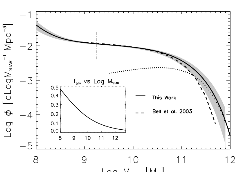
Figure 1.— The Galaxy Stellar Mass Function. The thick solid line shows the numerical results, which are almost perfectly matched by the analytic fitting formula [eq. (5)]. The dotted line gives the contribution of early-type galaxies. The shaded area represents the uncertainty due to the $\simeq 30\%$ error in the mean stellar mass to light ratio. The vertical dot-dashed line shows the stellar mass corresponding to $M_{r}=-18$. The dashed line shows the result by Bell et al. (2003). The inset illustrates the average fraction of gas as a function of the stellar mass.

The total GSMF, holding over the mass range $10^{8}\,M_{\odot}\lesssim M_{\mathrm{star}}\lesssim 10^{12}\,M_{\odot}$, is shown by the solid line in Fig. 1, where the shaded area corresponds to the 30% uncertainty in the mean MLR. This is a safe range to determine the GSMF as at lower masses the uncertainty in the LF grows while the increase in the total stellar mass density including $M_{\rm star}<10^{8}\,M_{\odot}$ is rather small, $<5\%$. The upturn at $M_{\mathrm{star}}\lesssim 3\times 10^{8}\,M_{\odot}$ corresponds to the appearance of the dwarf galaxy population, represented by the second term at r.h.s. of eq. (1). However the contribution in stellar mass density in the range $10^{8}\,M_{\odot}\lesssim M_{\mathrm{star}}\lesssim 10^{9}\,M_{\odot}$ is just $\sim$ 3% of the total. In the inset of Fig. 1 we have displayed the gas fraction as a function of the stellar mass. A very accurate analytical representation (actually indistinguishable from the solid line showing the numerical results) is provided by a Schechter function plus a power law term:

$${\mathrm{GSMF}(M_{\mathrm{star}})\,\mathrm{d}M_{\mathrm{star}}\over\hbox{Mpc}^{-3}}=\left({3\times 10^{-3}\over x^{1.16}\,e^{0.32\,x}}+{2.25\times 10^{-9}\over x^{3.41}}\right)\mathrm{d}x~{}\,,$$ (5)

where $x\equiv M_{\mathrm{star}}/6\times 10^{10}\,M_{\odot}$. The GBMF is easily computed by adding the appropriate gas contribution. Recent estimates of the GSMF and of the GBMF have been produced by Cole et al. (2001), Bell et al. (2003) and Baldry et al. (2004), exploiting 2dF, SDSS and Two Micron All Sky Survey data. The estimate by Bell et al. (2003) is shown by the dashed line in Fig. 1. The difference with our estimate is mainly due to the difference in adopted MLR. Bell et al. (2003) have derived their MLR by fitting the broad band SED with stellar population models. The mean MLR adopted here, based on kinematic determinations, is a factor of about $1.3$ higher at high luminosities, while at very low luminosities ($L_{r}\lesssim 5\times 10^{8}\,L_{\odot}$) it is about a factor of $2$ lower. However, the flatness of the GSMF at small masses conceals the difference in the MLR, while at large masses the almost exponential decline of the LF amplifies it. It is worth noticing that the determination of the MLR of low luminosity objects is hampered by many effects related to the episodic star formation history, to the presence of dust, to the irregularity of their shapes, and to the DM predominance.

Cole et al. (2001) presented estimates of the GSMF for two choices of the Initial Mass Function (IMF): Salpeter’s (1955) and Kennicutt’s (1983). For a Salpeter IMF their GSMF is consistent with ours, within our estimated uncertainties: the main difference is a $\simeq 30\%$ excess for $\log(M_{\rm star}/M_{\odot})\lesssim 10.5$. For a Kennicutt IMF, their GSMF drops for $M_{\rm star}$ about 0.2 dex lower than that by Bell et al. (2003). The estimate by Baldry et al. (2004) is close to that by Bell et al. (2003), as expected since they exploit very similar LFs and MLRs. All in all, methods based on kinematic measurements and on stellar population synthesis yield GSMFs and GBMFs in reasonable agreement, and establish a sound confidence interval.

Integrating the GSMF for $M_{\mathrm{star}}\gtrsim 10^{8}\,M_{\odot}$, the mass density parameter of baryons condensed in stars associated to late-type galaxies is found to be

$$\Omega_{\mathrm{star}}^{L}(\mathrm{kin})=(1.8\pm 0.4)\times 10^{-3}~{},$$ (6)

where the label “kin” indicates that the stellar mass of galaxies has been estimated using kinematic data. The corresponding neutral gas density amounts to $\sim 20\%$ of this value and it is concentrated in late-type, low mass systems with $M_{\mathrm{star}}\lesssim 5\times 10^{9}\,M_{\odot}$. Here and in the following eqs. (7) and (8), the errors reflect the uncertainties on the GSMF.

The star density parameter associated to early-type galaxies amounts to

$$\Omega_{\mathrm{star}}^{E}(\mathrm{kin})=(1.8\pm 0.6)\times 10^{-3}~{}.$$ (7)

It is well known that in early-types the amount of cold gas is negligible. Therefore, the overall local stellar mass density in galaxies with stellar masses in the range $10^{8}\,M_{\odot}\lesssim M_{b}\lesssim 10^{12}\,M_{\odot}$ is

$$\Omega_{\mathrm{star}}^{G}(\mathrm{kin})=(3.6\pm 0.7)\times 10^{-3}~{}.$$ (8)

This value is in good agreement with the recent estimates obtained through spectro-photometric galaxy models (Bell et al. 2003; Fukugita 2004; Fukugita & Peebles 2004). The contribution of the cold gas to the baryon density in galaxies is only $\sim 8\%$, and thus $\Omega_{b}^{G}\approx 1.08\Omega_{\mathrm{star}}^{G}$. This result confirms the well known conclusion that only a small fraction, $\lesssim 10\%$, of the cosmic baryons is today in stars and cold gas within galaxies. It is worth noticing that the star formation rate integrated over the cosmic history matches the overall local mass density in stars (see Nagamine et al. 2004). This mass density has been accumulated at high redshifts, $z\gtrsim 1$, for early-type galaxies and later on for late-types, as indicated by their respective stellar populations.

By subtracting from the cosmic matter density the contribution of baryons ($\Omega_{b}\leq 0.044$) and that of dark matter (DM) in groups and clusters of galaxies ($\Omega_{DM}^{\mathrm{C}}\approx 0.012$; Reiprich & Bohringer 2002), we obtain the DM mass density associated with galaxies $\Omega_{DM}^{G}\approx 0.21$, in excellent agreement with the determination by Fukugita & Peebles (2004). The average DM-to-baryon (essentially stars) mass fraction in galaxies turns out to be around $60$. This value must be compared with the cosmological ratio $R_{\mathrm{cosm}}=\Omega_{DM}/\Omega_{b}\approx 6$. In fact, in rich galaxy clusters the baryon mass, mostly in form of diffuse gas, and the DM halo mass have a ratio consistent with the “cosmic” DM to baryon ratio (see, e.g., Ettori, Tozzi & Rosati 2003). This evidences that the baryon fraction in galaxies decreases on average by a factor of about $10$ relative to the initial value, due to a number of astrophysical processes associated to the formation of these objects. In the following we will use the cosmic fraction $f_{\mathrm{cosm}}=1/R_{\mathrm{cosm}}\approx 0.17$.

3. The Galaxy Halo Mass Function and the $L$, $M_{\mathrm{star}}$ and $\sigma$ vs. halo mass relations

In order to investigate the relationships between the stellar and baryonic mass and the halo mass in galaxies in a one-to-one correspondence, the statistics of halos containing one single galaxy, the Galaxy Halo Mass Function (GHMF), has to be estimated. The overall HMF as found by numerical simulations (see, e.g., Jenkins et al. 2001; Springel et al. 2005) is well described by the Press & Schechter (1974) formula as modified by Sheth & Tormen (1999). However, in order to compute the GHMF, we have to deal with the problem of the halo occupation distribution (HOD; Peacock & Smith 2000; Berlind et al. 2003; Magliocchetti & Porciani 2003; Kravtsov et al. 2004; Abazajian et al. 2005). Two effects need to be taken into account: (i) the number of galaxies is actually larger than the number of DM halos, since a halo may contain a number of sub-halos, each hosting a galaxy, and (ii) the probability that very massive halos ($M_{h}\gtrsim 10^{12}$–$10^{13}\,M_{\odot}$) host a single giant galaxy drops rapidly with increasing halo mass.

To account for the effect (i) we use the results by Vale & Ostriker [2004; see their eqs. (1) and (3)] and we add to the HMF the subhalo mass function they have derived; we have checked that this procedure does not alter substantially the overall mass density in the galactic range. The subhalo MF by van den Bosch et al. (2005) is extremely close to the Vale & Ostriker one over the mass range of interest here, and gives essentially indistinguishable results. To account for effect (ii) we subtract from the HMF the halo mass function of galaxy groups and clusters. Estimates of the latter obtained by different groups (Girardi & Giuricin 2000; Martinez et al. 2002; Heinämäki et al. 2003; Pisani et al. 2003; Eke et al. 2006) are in reasonable agreement for $M_{h}\gtrsim 5\times 10^{12}\,M_{\odot}$. At lower masses the galaxy group mass function is very uncertain, and the recent study by Eke et al. (2006) finds a larger abundance of low luminosity groups than previously reported from smaller samples. On the other hand, from Fig. 8 (plus Fig. 15) of Eke et al. (2006), it looks plausible that galaxies dominate the MF for $M_{h}\lesssim 5\times 10^{12}\,M_{\odot}$. We stress, however, that, as discussed in the following, in the mass range considered here our results are only weakly sensitive to whether or not the galaxy group mass function is subtracted from the HMF.

Figure 2.— Galactic halo mass function. The heavy solid line shows the numerical results, obtained as described in Sect. 3, which are very accurately reproduced by the analytical approximation [eq. (9)]. We have plotted the results by Martinez et al. (2002) only for the halo mass range of interest here. Beyond ${M_{h}}\approx 2\times 10^{13}\,M_{\odot}$, the halo mass function is fully accounted for by groups and clusters of galaxies; as a consequence the GHMF goes to zero (shown as a dotted line beyond this limit).

The GHMF obtained subtracting from the HMF the group and cluster mass function estimated by Martinez et al. (2002) is shown in Fig. 2 and is well fit, in the range $11<\log M_{h}/M_{\odot}<13.2$, by a Schechter function

$$\mathrm{GHMF}(M_{h})~{}\mathrm{d}M_{h}={\theta\over\tilde{M}}\,\left({M_{h}\over\tilde{M}}\right)^{\alpha}\,e^{-(M_{h}/\tilde{M})}\,\mathrm{d}M_{h}~{},$$ (9)

with $\alpha=-1.84$, $\tilde{M}=1.12\times 10^{13}\,M_{\odot}$ and $\theta=3.1\times 10^{-4}\,\hbox{Mpc}^{-3}$. The fall off at high masses (where early-type galaxies dominate) mirrors the increasing probability of multiple occupation of mass halos found by Magliocchetti & Porciani (2003) for $M\gtrsim 3\times 10^{13}\,M_{\odot}$ (see also Zehavi et al. 2005). Weak lensing measurements also suggest an upper galaxy mass limit $M_{\mathrm{max}}\lesssim 3\times 10^{13}\,M_{\odot}$ (Kochanek & White 2001).

If two galaxy properties, $q$ and $p$, obey a monotonic relationship we can write

$$\mathrm{\Phi}(p){\mathrm{d}p\over\mathrm{d}q}\,\mathrm{d}q=\mathrm{\Psi}(q)\,\mathrm{d}q~{},$$ (10)

where $\Psi(q)$ is the number density of galaxies with measured property between $q$ and $q+\mathrm{d}q$ and $\Phi(p)$ is the corresponding number density for the variable $p$. The solution is based on a numerical scheme that imposes that the number of galaxies with $q$ above a certain value $\bar{q}$ must be equal to the number of galaxy halos with $p$ above $\bar{p}$ (see, e.g., Marinoni & Hudson 2002; Vale & Ostriker 2004), i.e.,

$$\int_{\bar{p}}^{\infty}\,\mathrm{\Phi}(p)\mathrm{d}p=\int_{\bar{q}}^{\infty}\,\mathrm{\Psi}(q)\,\mathrm{d}q~{}.$$ (11)

In the following $p\equiv M_{h}$ and $\Phi(p)\equiv\mathrm{GHMF}(M_{h})$, while the variable $q$ will be, in turn, the luminosity, the stellar mass, the velocity dispersion, and the central BH mass. It is worth noticing that in this way we establish a direct link between the specific galaxy property and the halo mass without any assumption or extrapolation of the DM density profile.

The monotonicity assumption is obviously critical for the applicability of the present approach. However direct evidence of monotonic relationships between several pairs of these quantities has been reported (Häring & Rix 2004; Ferrarese 2002; Baes et al. 2003; Tremaine et al. 2002), and additional data supporting the relationships derived here are discussed in the following.

We also implicitly assume that all galactic-size halos contain a visible galaxy. This assumption underlies all major semi-analytic models for galaxy formation, including the one by Granato et al. (2004), that we adopt as our reference model. The successes of this model in reproducing the redshift-dependent galaxy luminosity function in different wavebands provide strong support to this view.

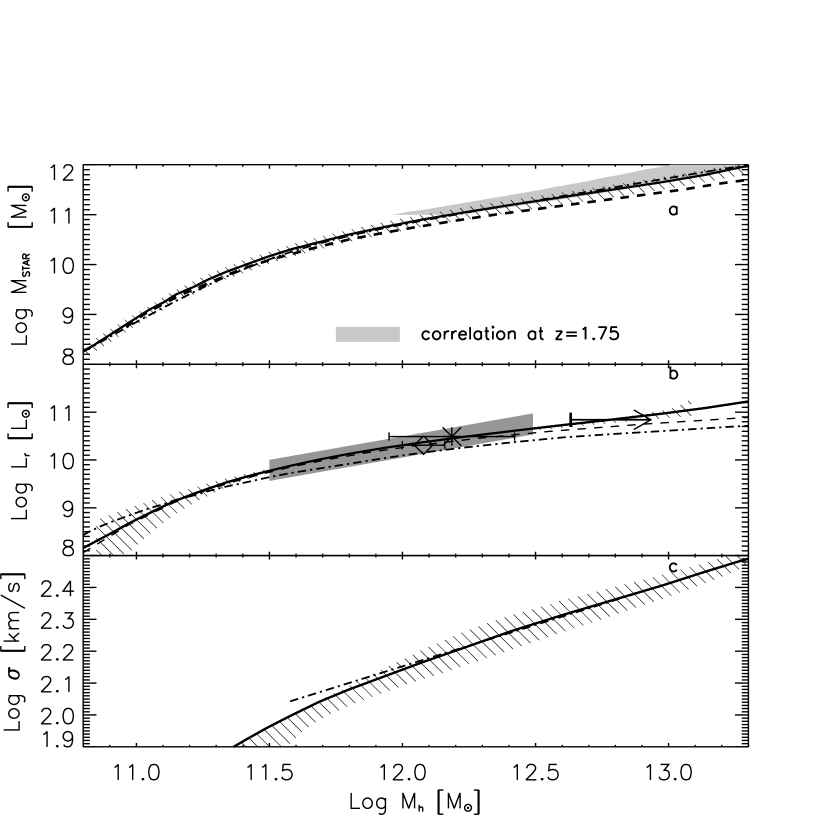
Figure 3.— ($a$) Mass in stars versus halo mass. The thick solid line shows the numerical results while the dot-dashed line (difficult to distinguish from the solid line) represents the analytic fitting formula [eq. (12)]. The dashed line has been obtained using the GSMF by Bell et al. (2003); the barred area represents the uncertainty associated to the mass to light ratio; the shaded area illustrates the result at $z=1.75$, based on data by Fontana et al. (2004). ($b$) $r^{*}$-band luminosity as a function of halo mass. Again, the thick solid line shows the numerical results and the analytic fitting formula [eq. (13)] is indistinguishable from it. The barred area represents the uncertainty associated to the LF (dominant at the low-mass end) and to the GHMF (dominant at the high-mass end); the thin dashed line is the numerical result obtained without removing the galaxy groups and clusters from the HMF; the dot-dashed line is the result by Vale & Ostriker (2004); the shaded region shows the result by Kleinheinrich et al. (2004); the arrow is from O’Sullivan & Ponman (2004); the diamond is from Hoekstra et al. (2004); the star is from Guzik & Seljak (2002). ($c$) $\sigma$–$M_{h}$ relation. As before, the thick solid line shows the numerical results while the dot-dashed line shows the analytic formula [eq. (15)] holding in the large $M_{h}$ limit. The barred area represents the uncertainty.

The result for the stellar mass, obtained setting $\mathrm{\Psi}(q)=\mathrm{GSMF}(M_{\mathrm{star}})$ [eq. (5)] is plotted in Fig. 3$a$. We find that its relationship with the host halo mass is well approximated by

$$M_{\mathrm{star}}\approx 2.3\times 10^{10}\,M_{\odot}\,\frac{(M_{h}/3\times 10^{11}\,M_{\odot})^{3.1}}{1+(M_{h}/3\times 10^{11}\,M_{\odot})^{2.2}}~{}.$$ (12)

The calculations for the baryonic mass is strictly analogous. Setting $\mathrm{\Psi}(q)=\phi(L_{r})$ [eq. (1)] we also derived the approximated behavior of the luminosity as a function of the halo mass

$$L_{r}\approx 1.2\times 10^{10}\,L_{\odot}\,\frac{(M_{h}/3\times 10^{11}\,M_{\odot})^{2.65}}{1+(M_{h}/3\times 10^{11}\,M_{\odot})^{2.00}}~{},$$ (13)

and of the halo mass as a function of luminosity

$${M_{h}\over 3\times 10^{11}\,M_{\odot}}=\left[\left(\frac{L_{r}}{1.3\times 10^{10}\,L_{\odot}}\right)^{0.35}+\left(\frac{L_{r}}{1.3\times 10^{10}\,L_{\odot}}\right)^{1.65}\right]~{}.$$ (14)

Both stellar mass and luminosity exhibit a double power law dependence on halo mass with a break around $M_{h,{\mathrm{break}}}\sim 3\times 10^{11}\,M_{\odot}$, corresponding to a luminosity $L_{r,{\mathrm{break}}}\sim 6\times 10^{9}\,L_{\odot}$.

The derivation of the $L_{r}$–$M_{h}$ relation is quite sensitive to uncertainties in the LF and in the GHMF. In the range $10^{9}\,L_{\odot}\lesssim L_{r}\lesssim 10^{11}\,L_{\odot}$ the LF is rather precisely known (see the comparison of different LF estimates in Fig. 1 of Shankar et al. 2004), while the effect of uncertainties in the GHMF becomes significant at large masses. On the whole, the $L_{r}$–$M_{h}$ relation is quite accurately determined in the range $10^{11}\,M_{\odot}\lesssim M_{h}\lesssim 10^{13}\,M_{\odot}$ (Fig. 3$b$). At low luminosities the errors on the LF rapidly increase, becoming a factor of about $2$ for $L_{r}\lesssim 3\times 10^{8}\,L_{\odot}$. In order to illustrate the consequences on the $L_{r}$–$M_{h}$ relation, we have computed it using the $1\,\sigma$ upper and lower boundaries of the LF by Nakamura et al. (2003). In the former case, the low-luminosity portion of the $L_{r}$–$M_{h}$ relation flattens from a slope of $\sim 2.6$ to $\sim 1.9$; in the latter case, it decreases almost exponentially. Therefore, the extrapolation of the above relationships to $L_{r}\ll 10^{9}\,L_{\odot}$ and, correspondingly, to $M_{h}\ll 10^{11}\,M_{\odot}$ must be taken cautiously. Of course, the same conclusion holds for relationships involving other statistics of galaxies and of their host halos. This emphasizes the need of a precise determination of the low luminosity end of the LF.

In Fig. 3$b$ our estimate of the $L_{r}$ vs. $M_{h}$ relation is compared with observational results for galaxies whose $M_{h}$ could be derived based on two different methods: (i) an X-ray-based mass model of the isolated elliptical galaxy NGC 4555 (O’Sullivan & Ponman 2004), in which the gravitational potential is known up to about $1/8$ of the virial radius (the mass within this radius is shown as a lower limit in Fig. 3$b$); (ii) weak-lensing observations that provide the shear field around a number of galaxies of average luminosity $L$, from which it is possible to infer the projected mass density and eventually to extrapolate the virial mass by assuming a DM profile (Guzik & Seljak 2002; Kleinheinrich et al. 2004; Hoekstra et al. 2004). In Fig. 3$b$ we also show for comparison the $L_{r}$ vs. $M_{h}$ relation obtained from eq. (10) setting $\Phi(p)=HMF(M_{h})$. It is worth noticing that if the group and cluster MF is not subtracted from the HMF, our results vary only at high masses, and the changes do not exceed 0.2 dex up to $M_{h}\simeq 2\times 10^{13}\,M_{\odot}$.

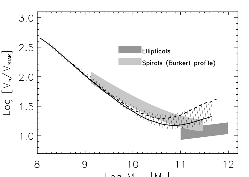
Figure 4.— Halo to stellar mass ratio as a function of the stellar mass. The solid line is the result of numerical calculations using eq. (11) with $\Phi(p)\equiv\mathrm{GHMF}(M_{h})$ and $\mathrm{\Psi}(q)\equiv\mathrm{GSMF}(M_{\mathrm{star}})$, as given by [eq. (5)]; the barred area represents the uncertainty associated to the mass to light ratio. The dashed line has been obtained using the GSMF by Bell et al. (2003). The Cole et al. (2001) GSMF with a Salpeter (1955) IMF yields results very close to ours. The dark shaded area represents the data on giant elliptical galaxies by Gerhard et al. (2001); the light shaded area represents data on spiral galaxies by Persic, Salucci & Stel (1996) and Salucci & Burkert (2000).

As a further check, our estimate of the ratio $M_{h}/M_{\mathrm{star}}$ as a function of $M_{\mathrm{star}}$, is compared in Fig. 4 with estimates derived by extending to the virial radius the inner mass models of a number of giant ellipticals (Gerhard et al. 2001) and spirals (Persic, Salucci & Stel 1996; Salucci & Burkert 2000). We stress that these results require extrapolations to the virial radius of the density profile, assumed to have the Navarro, Frenk & White (1996) shape, while our estimate does not need any assumption on DM density profile. It is apparent that these independent results are in nice agreement with our findings.

The dependence of the luminosity on the halo mass has been investigated also by Vale and Ostriker (2004); their result is also shown in Fig. 3$b$. They exploited the 2dF galaxy luminosity function in the $b_{J}$-band (Norberg et al. 2002), extrapolating it beyond the range of magnitudes where it was defined. The difference in the $L_{r}$-$M_{h}$ relation between our estimate and theirs is due to the steeper slope of the LF adopted by them. There is also a small difference in the normalization of the LF, but this is of minor importance.

At high masses the direct comparison of the galaxy LF to the halo plus subhalo number density [cf. their eq. (9)] results in a slight flattening of the relation (dot-dashed curve for Vale & Ostriker, dashed curve for our calculations). As Vale and Ostriker (2004) pointed out, in this way the mass term refers to the entire halo hosting the group or the cluster and not to just the galaxy halo.

Guzik & Seljak (2002) modelled the galaxy-galaxy lensing trying to separate the central galactic contributions from contributions of the surrounding groups and clusters. Their model applied to the SDSS data on galaxy lensing yields $M_{h}/L_{r}\approx 50\,M_{\odot}/L_{\odot}$ at the characteristic luminosity $3\times 10^{10}\,L_{\odot}$ for early-type galaxies, in keeping with our results. They also found a luminosity dependence $M_{h}\propto L^{1.4\pm 0.2}$, compatible with the high-luminosity slope of eq. (14). However, we find that, at low luminosities, the slope significantly flattens toward a dependence $M_{h}\propto L^{0.35}$, while Guzik & Seljak (2002) assume a single power law relation.

Van den Bosch et al. (2003, 2005) computed the conditional luminosity function of early- and late-type galaxies, a statistics linking the distribution of galaxies to that of the DM. They concluded that the MLR has a minimum $M_{h}/L_{r}\sim 45-70\,M_{\odot}/L_{\odot}$ at $M_{h}\sim 2-4\times 10^{11}\,M_{\odot}$, consistent with eq. (14).

Marinoni & Hudson (2002) investigated the MLRs of the virialized systems, which include galaxies, groups and clusters. By comparing their luminosity function to the $\Lambda$CDM halo mass function, they concluded that the MLR has a broad minimum around $L_{B}\approx 3\times 10^{10}\,L_{\odot}$. The slopes at low and high luminosity are $-0.5$ and $+0.5$, respectively. Our slope is similar at low masses, where practically all virialized systems are galaxies and thus the comparison is meaningful. The studies by Eke et al. (2004, 2006) of the variation of the MLR with size of galaxy groups is fully consistent with a minimum at approximately the same luminosity.

By comparing the HMF and the LF, as we have done for local galaxies, it is possible to infer the $M_{\mathrm{star}}$–$M_{h}$ relation even at substantial redshifts. For the GSMF we use a simple linear fit [$\log(\phi(M_{\rm star})/\hbox{Mpc}^{3})=-1.7\log(M_{\rm star}/M_{\odot})+16.1$, holding for $11\leq\log(M_{\rm star}/M_{\odot})\leq 12$] to the data by Fontana et al. (2004) at $\bar{z}=1.75$, and we approximate the GHMF with the HMF computed at the same redshift. The result, shown by the shaded area in Fig. 3$a$, has to be taken as an upper limit since we have neglected the contribution of galaxy groups to the HMF. Clearly, our estimate becomes increasingly uncertain as we approach the upper limit of the interval where GSMF is observationally estimated; this is reflected in the increased width of the shaded area. Nevertheless, the $M_{\mathrm{star}}$–$M_{h}$ relation at $\bar{z}=1.75$ turns out to be quite close to the local one, indicating that for large galaxies the $M_{\mathrm{star}}$–$M_{h}$ relation was already in place at redshift $z\gtrsim 1$ in line with the anti-hierarchical baryon collapse scenario developed by Granato et al. (2001; 2004).

Sheth et al. (2003) estimated the Velocity Dispersion Function (VDF) of spheroidal galaxies using a sample drawn from the SDSS survey and have built a simple model for the contribution to the VDF of the bulges of spirals, which dominate at low velocity dispersions. Their estimate covers the range $80$ km s${}^{-1}\leq\sigma\leq 400$ km s^-1. Comparing the global VDF (including both early and late type galaxies, as shown in Fig. 6 of Sheth et al.), and the GHMF with the same technique presented above [cf. eqs. (10) and (11)], we can derive the $\sigma$–$M_{h}$ relationship shown in panel (c) of Fig. 3. For $M_{h}\geq 6.3\times 10^{11}$, the relationship is accurately represented by a simple power-law:

$$\sigma\approx 110\,\mathrm{km\,s}^{-1}\,\left({M_{h}\over 6.3\times 10^{11}\,M_{\odot}}\right)^{1/3}~{},$$ (15)

while it steepens for lower halo masses. The uncertainties strongly increase for $\sigma\lesssim 80$ km s^-1, corresponding to $M_{h}\lesssim 10^{11}\,M_{\odot}$. Note that these relationships must break down in the low-$\sigma$ (and low-$M_{h}$) regime. In fact, the close match found by Cirasuolo et al. (2005) between the VDF and the virial velocity function (derived from the halo mass distribution function integrated over redshift) indicates that halos more massive than $M_{h}\sim 10^{11}\,M_{\odot}$ are generally associated to spheroidal galaxies or to later type galaxies with bulge velocity dispersions $\sigma\gtrsim 80$ km s^-1. On the other hand, the fraction of galactic halos associated to essentially bulgeless late-type galaxies must increase with decreasing $M_{h}$, so that the integral of the VDF deviates from that of the GHMF and eq. (11) no longer applies.

Figure 5.— Fraction of primordial gas turned into stars as a function of halo mass. The solid line has been obtained numerically from eq. (11) with $\Phi(p)\equiv\mathrm{GHMF}(M_{h})$ and $\mathrm{\Psi}(q)\equiv\mathrm{GSMF}(M_{\mathrm{star}})$, as given by [eq. (5)]; the barred area represents the uncertainty associated to the mass to light ratio. The dashed line has been obtained using the GSMF by Bell et al. (2003). We have set $f_{\mathrm{cosm}}=1/6$.

Figure 5 shows the ratio of the mass in stars to the initial baryon mass associated with each halo, assumed to be $M_{b,i}=f_{\mathrm{cosm}}M_{h}$, as a function of $M_{h}$. It illustrates the “inefficiency” of galaxies, especially of those of low halo mass, in retaining baryons. As discussed in § 5, the shape of the $M_{\rm star}/f_{\rm cosm}M_{h}$ can be understood in terms of feedbacks: at low masses the SN feedback is very efficient in removing the gas, thus quenching the star formation; moving toward higher masses (for $\log(M_{\rm BH})\gtrsim 7.5$, corresponding to $\log(M_{h}\gtrsim 12)$) the AGN feedback becomes more and more powerful, to the point of sweeping out most of the initial baryons.

Our result is at odds with the claim by Guzik & Seljak (2002) of a high efficiency, up to $75\%$, in turning primordial gas into stars. However, the claim is based on a MLR $M_{h}/L_{i}\approx 17h\,M_{\odot}/L_{\odot}$ in the $i^{\prime}$ band for late-type galaxies, a factor of 3 lower than the value found for the early-type ones. As the authors themselves point out, the statistical significance of this result is marginal, due to the weak lensing signal for the fainter late-type galaxy sample. The GSMFs by Cole et al. (2001) and Bell et al. (2003) yield similar efficiencies, which are very close to our estimates for relatively low halo masses, but lower for large masses, yet within the estimated uncertainties.

4. Black hole vs. halo mass

The relation between the central supermassive black hole and the halo mass $M_{h}$ is relevant in the framework of theories for the origin and evolution of both galaxies and AGNs (Silk & Rees 1998; Monaco, Salucci & Danese 2000; Granato et al. 2001; Ferrarese 2002; Granato et al. 2004). To constrain such relation we adopted the procedure presented in the previous Section [eqs. (10) and (11)], replacing the function $\Psi(q)$ with the local BH mass function (Shankar et al. 2004). We assume that each galactic halo hosts just one supermassive BH. Our result is shown in Fig. 6, where the barred area illustrates the errors due to the observational uncertainties on the BH mass function, as estimated by Shankar et al. (2004). We find good agreement, within the estimated uncertainties, with the predictions of the Granato et al. (2004) model.

The relationship can be approximated by

$$M_{\rm BH}\approx 6\times 10^{6}\,M_{\odot}\,\frac{(M_{h}/2.2\times 10^{11}\,M_{\odot})^{3.95}}{1+(M_{h}/2.2\times 10^{11}\,M_{\odot})^{2.7}}~{}.$$ (16)

Again a double power law with a break at $M_{h}\sim 3\times 10^{11}\,M_{\odot}$ is a very good representation of our results. At the high mass end, the BH mass is nearly proportional to the halo mass ($M_{\rm BH}\propto M_{h}^{1.25}$), while at low masses the relation steepens substantially ($M_{\rm BH}\propto M_{h}^{3.95}$).

In Fig. 6 we also compare our estimate of the $M_{\rm BH}$–$M_{h}$ relation with that of Ferrarese (2002), who first investigated this issue from an observational point of view. She derived a power-law relationship between the bulge velocity dispersion and the maximum circular velocity, $v_{c}$, for a sample of spiral and elliptical galaxies spanning the range $100\lesssim v_{c}\lesssim 300$ km s^-1, and combined it with the relationship between $v_{c}$ and the virial velocity, $v_{\rm vir}$ based on the numerical simulations by Bullock et al. (2001) and with the $M_{h}$–$v_{\rm vir}$ relationship given by the $\Lambda$CDM model of the latter authors for a virialization redshift $z_{\rm vir}\sim 0$, to obtain a $M_{h}$–$\sigma$ relation. Coupling it with one version of the observed BH mass vs. stellar velocity dispersion relationship ($M_{\rm BH}\propto\sigma^{4.58}$) she obtained $M_{\rm BH}\propto M_{h}^{\alpha}$, with $\alpha=1.65$–1.82. Baes et al. (2003) with the same method, but assuming $M_{\rm BH}\propto\sigma^{4.02}$ and with new velocity dispersion measurements of spiral galaxies with extended rotation curves, yielding a slightly different $v_{c}$-$\sigma$ relation, found $M_{\rm BH}\propto M_{h}^{1.27}$. It is apparent from Fig. 6 that our result differs substantially in normalization, while the high-mass slope is remarkably close to that obtained by Baes et al. (2003). It should be noted that the $M_{h}$–$V_{\rm vir}$ relation depends on the virialization redshift. For $z_{\rm vir}\simeq 3$ [the median virialization redshift for galaxies with velocity dispersions in the range probed by Ferrarese and Baes et al., according to the analysis by Cirasuolo et al. (2005; see their Fig. 1)], its coefficient would be a factor of $\simeq 4.25$ lower than that used by Ferrarese (2002) and Baes et al. (2003) and the coefficients of the $M_{\rm BH}\propto M_{h}$ relations would be larger by a factor of $\simeq 5.6$ in the case of eq. (6) of Ferrarese(2002) or of $\simeq 4$ in the case of Baes et al. (2003), bringing them much closer to ours. In fact, as suggested by Loeb & Peebles (2003) and shown in details by Cirasuolo et al. (2005), the velocity dispersion of the old stellar population (whose mass is related to the central BH mass) is closely linked to halo mass and characteristic velocity at the virialization redshift.

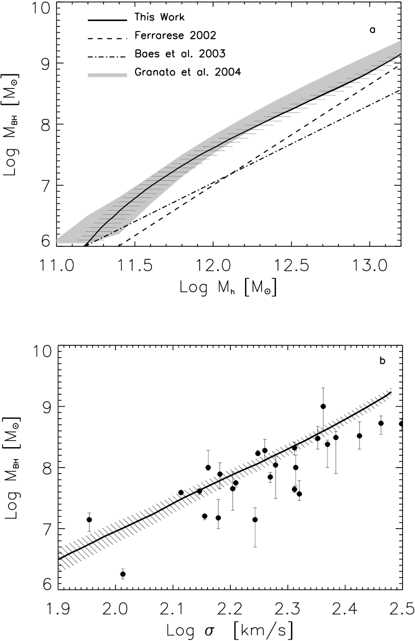
Figure 6.— Upper panel: super-massive BH mass versus halo mass. The solid line has been obtained numerically from eq. (11) with $\Phi(p)\equiv\mathrm{GHMF}(M_{h})$ and $\mathrm{\Psi}(q)$ is the local super-massive BH mass function estimated by Shankar et al. (2004). The dashed line is the relation by Ferrarese et al. [2002; her eq. (6)]; the dot-dashed line is the relation by Baes et al. (2003). The shaded area represents the prediction of the Granato et al. (2004) model. Lower panel: $M_{\rm BH}$–$\sigma$ relation obtained combining the $M_{\rm BH}$–$M_{h}$ relation (upper panel) with the $\sigma$–$M_{h}$ relation (panel (c) of Fig. 3). The data are from Ferrarese & Ford (2005). In both panels the barred area reflects the uncertainty associated to the BH Mass Function.

As a consistency test, we have combined the $M_{\rm BH}$–$M_{h}$ relation, shown in the upper panel of Fig. 6, with the $\sigma$–$M_{h}$ relation, shown in panel (c) of Fig. 3, to obtain the $M_{\rm BH}$–$\sigma$ relation (see Ferrarese & Ford 2005 for a review), which turns out to be consistent with the data, as shown by the lower panel in Fig. 6.

5. Feedback from stars and AGNs

The dependence of the star and BH masses on the halo mass found in the previous Section, suggests that different physical mechanisms are controlling the star formation and the BH growth above and below $M_{h,{\mathrm{break}}}\sim 3\times 10^{11}\,M_{\odot}$, corresponding to $M_{\mathrm{star}}\sim 1.2\times 10^{10}\,M_{\odot}$ after eq. (12), and to $L_{r}\sim 5\times 10^{9}\,L_{\odot}$ (or $M_{r}\sim-19.6$) after eq. (13). It is worth noticing that the analysis of a huge sample of galaxies drawn from the SDSS shows that around $M_{\mathrm{star}}\approx 2$–$3\times 10^{10}\,M_{\odot}$ and $M_{r}\sim-19.8$ there is a sort of transition in the structure and stellar ages of galaxies (Kauffmann et al. 2003; Baldry et al. 2004).

The efficiency of star formation within galactic halos of different masses is the result of several processes. The most important are: (i) the cooling of the primordial gas within the virialized halos (White & Rees 1978); (ii) the injection of large amounts of energy into the ISM by supernova explosions (Dekel & Silk 1986; White & Frenk 1991; Granato et al. 2001; Romano et al. 2002) and by the central quasar (Silk & Rees 1998; Granato et al. 2001, 2004; Lapi et al. 2005). All these processes have been implemented in the model of Granato et al. (2004). A simplified, analytical rendition of this model is presented in the Appendix A.

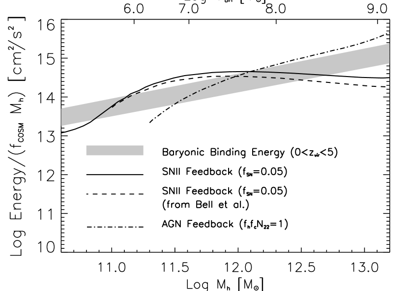
Figure 7.— Specific energy feedback from stars and AGNs compared to the baryon specific binding energy within the host halo, as a function of the halo mass. The solid line refers to our estimate of the SN feedback while the dashed line is the SN feedback obtained using the GSMF of Bell et al. (2003). The dot-dashed line is our estimate of the AGN feedback. The shaded area shows the specific binding energy of the gas in the DM potential well, for virialization redshifts $0\leq z_{\mathrm{vir}}\leq 5$.

The impact of stellar and AGN feedback is illustrated by Fig. 7. The binding energy of baryons in the DM potential well per unit baryonic mass as a function of the halo mass [cf. eq. (A4)] for $0\leq z_{\mathrm{vir}}\leq 5$ is shown by the shaded area. To compute the overall energy per unit baryonic mass injected in the gas by supernovae ($E_{\mathrm{star}}$) and by AGNs ($E_{\rm AGN}$), we have exploited eqs. (A9) and (A14), respectively, where $M_{\mathrm{star}}$ and $M_{\rm BH}$ as functions of the halo mass are given by eqs. (12) and (16), respectively. Then we divided the overall energies by the initial baryon mass $M_{b,i}=f_{\mathrm{cosm}}M_{h}$. Figure 7 shows that for large masses the gas can be efficiently removed by the AGN feedback which overwhelms the binding energy. For small masses the supernova feedback dominates but appears to be insufficient to remove the gas associated to the host halo, due to the above mentioned problem that the observed $M_{\mathrm{star}}$–$M_{h}$ relation inferred from the data exhibits a too steep low-mass slope. The flattest slope allowed by the data, discussed in § 3, would largely alleviate, but not completely overcome, this problem.

The relative importance of the two feedbacks depends on their efficiency in transferring the available energy to the gas. It is interesting that with the efficiencies used in Fig. 7 the crossing point is quite close to $M_{h,{\mathrm{break}}}\approx 3\times 10^{11}\,M_{\odot}$. As discussed by Granato et al. (2004) and Cirasuolo et al. (2005), a more accurate evaluation of the efficiencies can be obtained by fitting statistics of galaxies and of AGNs, such as LFs at low and high redshift, the Faber and Jackson relation, and the local BH mass function.

A more quantitative insight into the role of the key ingredients of the model is provided by the analytic calculations presented in the Appendix A. So long as the star formation rate obeys eq. (A2), the mass in stars at a the present time $t$, assumed to be $>>t_{c}$, is given, after eq. (A8), by:

$$M_{\mathrm{star}}\propto f_{\mathrm{surv}}\,{f_{\mathrm{cosm}}M_{h}\over 1-R+\alpha}~{},$$ (17)

where $f_{\mathrm{surv}}$ is the fraction of stars that survive up to now.

For large halo masses, where the stellar feedback is less efficient ($\alpha\lesssim 1$), the quantity $1-R+\alpha$ is a slowly decreasing function of the halo mass, so that $M_{\mathrm{star}}$ is approximately proportional to $M_{h}$. However, in this case, the fraction of gas turned into stars is controlled by the AGN feedback, which, as shown by the full treatment by Granato et al. (2004), for $M_{h}\gtrsim 3\times 10^{11}\,M_{\odot}$ expels an approximately constant fraction of the initial gas, thus preserving the approximate proportionality between $M_{\mathrm{star}}$ and $M_{h}$, in agreement with eq. (12).

The effective optical depth, which rules the flow of the cold gas into the reservoir around the BH [cf. eq. (A10)], is large ($\tau\gtrsim 1$) for large galaxies, implying, after eq. (A11), $M_{\rm BH}\approx 1.2\times 10^{-3}\,M_{\mathrm{star}}$. As a consequence, in the high mass limit, the BH mass must have a dependence on the halo mass very similar to that of the stellar mass, in agreement with eq. (16).

For $M_{h}\ll 10^{12}\,M_{\odot}$ the dominant term in the denominator in the right-hand side of eq. (17) is the effective efficiency of the SN feedback, $\alpha\propto M_{h}^{-2/3}$ [cf. eq. (A6)]. Therefore we get

$$M_{\mathrm{star}}\propto f_{\mathrm{surv}}\,M_{h}^{5/3}~{}.$$ (18)

This limiting dependence has been derived theoretically also by Dekel & Woo (2003) with similar assumptions. On the other hand, such a relation is significantly flatter than that inferred from the data [cf. eq. (12) and Fig. 7]. Possible explanations may be that in less massive halos the initial baryon fraction is lower by effect of reheating of the intergalactic medium, hindering the infall of baryons into the shallower potential wells, or that the SN efficiency in removing the gas is higher. However, the difference must not be overemphasized, in view of the large uncertainties on the shape of the $M_{\mathrm{star}}$–$M_{h}$ and $M_{h}$-$L_{r}$ relations at low masses/luminosities, induced by our poor knowledge of the low-luminosity portion of the LF. As discussed in § 3, the data are consistent also with a flatter relation ($M_{\mathrm{star}}\propto M_{h}^{1.9}$).

Since in the mass range $M_{h}\lesssim 10^{11}\,M_{\odot}$ the optical depth is small ($\tau\ll 1$), from eqs. (A11) and (A12) we obtain:

$$M_{\rm BH}\propto M_{\mathrm{star}}\,\tau\propto M_{h}^{7/3}~{}.$$ (19)

Thus this simple model predicts that the low mass slope of the $M_{\rm BH}$–$M_{h}$ relation is steeper than that of the $M_{\mathrm{star}}-M_{h}$ relation, because of the decrease of the optical depth with mass $\tau\propto M_{h}^{2/3}$, entailing a lower capability of feeding the reservoir around the BH. Interestingly, a steepening by approximately this amount is also found from our analysis of observational data [cf. eqs. (12) and (16)].

6. Conclusions

We computed the stellar and baryon mass function in galaxies exploiting $M/L$ ratios for stars and gas derived from galaxy kinematics. The results turn out to be in agreement with previous analyses based on stellar population models. The total baryonic mass density in galactic structures amounts to $\Omega_{b}^{G}\approx(3.6\pm 0.7)\times 10^{-3}$, of which $\sim 40\%$ resides in late-type galaxies. This result confirms the well-known conclusion that only a fraction $\lesssim 10\%$ of the cosmic baryons are presently in stars and cold gas within galaxies.

The present-day galaxy halo mass function, i.e., the number density of halos of mass $M_{h}$ containing a single baryonic core, has been estimated by adding the subhalos to the halo mass function and by subtracting the contributions from galaxy groups and clusters. Such subtraction, which is required to single out galactic halos, has however a minor effect over the mass range of interest here.

Approximated analytic relationships between the halo mass, $M_{h}$, the mass in stars, $M_{\mathrm{star}}$, and the $r^{*}$-band luminosity, $L_{r}$, have been obtained from the functional equations $\mathrm{\Phi}[>M_{h}(q)]=\mathrm{\Psi}(>q)$, where $\mathrm{\Phi}(>M_{h})$ is the number density of galactic halos larger that $M_{h}$ and $\mathrm{\Psi}(>q)$ is the number density of galaxies with either stellar mass greater than $M_{\mathrm{star}}$ or luminosity greater than $L_{r}$. The results are in good agreement with $M_{h}/L_{r}$ ratios inferred through X-ray mapping of the gravitational potential and through gravitational lensing. Both relations exhibit a double-power law shape with a break around $M_{h,{\mathrm{break}}}\approx 3\times 10^{11}\,M_{\odot}$, corresponding to $M_{\mathrm{star},\mathrm{break}}\approx 1.2\times 10^{10}\,M_{\odot}$ and to an absolute magnitude $M_{r,{\mathrm{break}}}\approx-19.6$. A transition at about the same magnitude in the galaxy properties has been evidenced by Kauffmann et al. (2003) and Baldry et al. (2004).

An additional interesting outcome of our analysis is that the $M_{\mathrm{star}}$–$M_{h}$ relation is already established at redshift $z\approx 1.7$, in line with the theoretical expectation of the anti-hierarchical baryon collapse scenario (Granato et al. 2004).

Applying the same technique to the local velocity dispersion function of galaxies and to the black hole mass function, we have also computed the $\sigma$–$M_{h}$ and $M_{\rm BH}$–$M_{h}$ relationships. The former is quite close to a single power law $\sigma\propto M_{h}^{1/3}$. The latter is again a double power law breaking approximately at $M_{h,{\mathrm{break}}}$, corresponding to $M_{\rm BH}\sim 9\times 10^{6}\,M_{\odot}$. The associated velocity dispersion, $\sigma\simeq 88$ km s^-1, is very close to the first estimate of the critical velocity dispersion for the gas removal by SN explosions given by Dekel & Silk (1986), who found a critical halo velocity $V_{\mathrm{crit}}\sim 120$ km s^-1, corresponding to a critical velocity dispersion $\sigma_{\mathrm{crit}}\sim 80\,\hbox{km}\,\hbox{s}^{-1}$.

As a test of our results, we combined the $M_{\rm BH}$–$M_{h}$ relation [eq. (16)] with the $\sigma$–$M_{h}$ relation [eq. (15)]; as shown by the lower panel of Fig. 6, the resulting $M_{\rm BH}$–$\sigma$ relation is consistent with the observational data.

The relationships we have obtained are model-independent and can be interpreted in terms of feedback effects by supernovae and AGNs in galactic structures. We also presented a simple feedback model, which nicely reproduces the approximate proportionalities $M_{\rm BH}\propto M_{\mathrm{star}}\propto M_{h}$ observed in the high mass range, and the break of these relationships at $M_{h,{\mathrm{break}}}\approx 3\times 10^{11}\,M_{\odot}$.

At low masses, the $M_{\mathrm{star}}$–$M_{h}$ relation derived here ($M_{\mathrm{star}}\propto M_{h}^{3.1}$) is steeper than that yielded by the model ($M_{\mathrm{star}}\propto M_{h}^{5/3}$), and would imply that only a tiny fraction of the baryons initially associated with the halo remains within it in the form of stars (and we know that the gas does not add much to the baryon content of galaxies). On the other hand, if the amount of stars formed is so low, for a standard Salpeter IMF the energy injected by SN explosions is insufficient to expel the residual gas if the baryon fraction is close to the cosmic value. Thus, if the slope of the $M_{\mathrm{star}}$–$M_{h}$ relation really is as steep as its face value suggests, we must conclude that either the initial baryon fraction in low-mass galaxies was substantially lower than the cosmic value (due, e.g., to a pre-heating of the intergalactic medium hampering the infall of baryons into shallow potential wells) or that the SN feedback in these objects was substantially stronger than in more massive galaxies. As discussed in § 3, however, the uncertainties on the low luminosity portion of the LF are large enough to allow for a flatter slope, closer to the model prediction and almost sufficient to grant the gas removal by SN feedback.

The errors shown in the figures mostly reflect uncertainties in the $M/L$ ratio. We must not forget however, other error sources. For example, Fig. 3$b$ shows that different choices for the GHMF yield a systematic difference in the results, that, at the high-mass end, become comparable to the scatter considered in the same figure. Further uncertainties come from estimates of the GSMF; these are illustrated, in Figs. 3,  4,  5, and  7, by comparisons with results obtained using the GSMF by Bell et al. (2003). Nevertheless, our approach provides results consistent with observations, and have comparable uncertainties. Moreover, since our approach bypasses any assumption on the DM profile, it could provide a valuable tool to discriminate among the different models of DM mass distribution in galaxies.

Our analysis has shown that the relationships presented above bear the imprint of the processes ruling the galaxy formation and evolution. Models should eventually comply with them.

Appendix A A simple feedback model

The rate at which the gas mass $M_{\mathrm{inf}}$ falls toward the central star forming regions can be written as

$$\dot{M}_{\mathrm{inf}}(t)=-\frac{M_{\mathrm{inf}}(t)}{t_{c}}~{}.$$ (A1)

The infalling gas mass thus declines exponentially $M_{\mathrm{inf}}(t)=M_{\mathrm{inf}}(0)\,\exp(-t/t_{c})$, where $t_{c}=\max[t_{\mathrm{cool}}(r_{\mathrm{vir}}),t_{\mathrm{dyn}}(r_{\mathrm{vir}})]$ is the maximum between the cooling and the dynamical time at the virial radius, while $M_{\mathrm{inf}}(0)=f_{\mathrm{cosm}}\,M_{h}$ is the initial gas mass.

The time derivative of the cold, star forming gas mass is given by

$$\dot{M}_{\mathrm{cold}}(t)=\frac{M_{\mathrm{inf}}(t)}{t_{c}}-\psi(t)+R\psi(t)-\alpha\psi(t)~{},$$ (A2)

where $\psi(t)\equiv\dot{M}_{\mathrm{star}}$ is the Star Formation Rate (SFR), $R$ is the fraction of mass restituted by evolved stars ($R\approx 0.3$ for a Salpeter IMF), and

$$\alpha=\frac{N_{SN}\,\epsilon_{SN}\,E_{SN}}{E_{B}}$$ (A3)

is effective efficiency for the removal of cold gas by the supernova feedback. Here $N_{SN}$ is the number of SNe per unit solar mass of condensed stars, $\epsilon_{SN}\,E_{SN}$ the energy per SN used to remove the cold gas, and $E_{B}$ the binding energy of the gas within the DM halo, per unit gas mass. Following Zhao et al. (2003) and Mo & Mao (2004), the latter quantity can be written as

$$E_{B}=\frac{1}{2}\,V_{\mathrm{vir}}^{2}\,f(c)(1+f_{\mathrm{cosm}})~{},$$ (A4)

where $V_{\mathrm{vir}}$ is the circular velocity at the virial radius for a halo mass $M_{h}$, $f(c)\approx 1$ is a weak function of the concentration $c$, and we have assumed that, initially, the gas fraction is equal to the cosmic baryon to dark-matter mass density ratio, $f_{\mathrm{cosm}}$. Taking into account the dependence of $V_{\mathrm{vir}}$ on the halo mass and redshift, we get, for $z\gtrsim 1$:

$$E_{B}\approx 3.2\times 10^{14}\left(\frac{1+z}{4}\right)\left(\frac{M_{h}}{10^{12}\,M_{\odot}}\right)^{2/3}\,(\mathrm{cm/s})^{2}~{}.$$ (A5)

The effective efficiency is well approximated by

$$\alpha\approx 1.2\,\left(\frac{N_{SN}}{8\times 10^{-3}}\right)\,\left(\frac{\epsilon_{SN}}{0.1}\right)\,\left(\frac{E_{SN}}{10^{51}\hbox{erg}}\right)\,\left(\frac{1+z}{4}\right)^{-1}\,\left(\frac{M_{h}}{10^{12}\,M_{\odot}}\right)^{-2/3}~{}.$$ (A6)

Further setting

$$\psi(t)=\frac{M_{\mathrm{cold}}}{t_{\mathrm{star}}}~{},$$ (A7)

$t_{\mathrm{star}}$ being the star-formation timescale, eq. (A2) is easily solved for $M_{\mathrm{cold}}(t)$. The mass $M_{\mathrm{star}}$ cycled through stars is then straightforwardly obtained, using eq. (A7):

$$M_{\mathrm{star}}(t)=\int_{0}^{t}\psi(t^{\prime})dt^{\prime}=\frac{M_{\mathrm{inf}}(0)}{\gamma}\left[1-\frac{s\gamma}{s\gamma-1}\,\exp(-t/t_{c})+\frac{1}{s\gamma-1}\,\exp(-s\gamma t/t_{c})\right]~{},$$ (A8)

where $\gamma=1-R+\alpha$. In the above formula, $s=t_{c}/t_{\mathrm{star}}\gg 1$, since we expect that in the central, clumpy regions the cooling and dynamical times are shorter than $t_{c}$, which is estimated at the virial radius. The mass in stars at the present time only includes the fraction $f_{\mathrm{surv}}$ of stars still surviving: $M_{\mathrm{star}}^{\mathrm{now}}=f_{\mathrm{surv}}\,M_{\mathrm{star}}(t_{\mathrm{now}})$. The survived fraction depends on the IMF and on the history of star formation; as a reference, for a Salpeter IMF after about 10 Gyr from a burst we have $f_{\mathrm{surv}}\approx 0.6$. If we assume that most of the stellar feedback comes from SN explosions, then the total energy injected into the gas is given by

$$E_{\mathrm{star}}=\epsilon_{SN}\,E_{SN}\,N_{SN}\,M_{\mathrm{star}}\approx 8\times 10^{58}\,\left(\frac{\epsilon_{SN}}{0.1}\right)\,\left(\frac{E_{SN}}{10^{51}\hbox{erg}}\right)\,\left(\frac{N_{SN}}{8\times 10^{-3}}\right)\,\frac{M_{\mathrm{star}}}{10^{11}\,M_{\odot}}~{}\mathrm{erg}.$$ (A9)

As long as a significant amount of cool gas is present in the central regions, we can imagine that there are mechanisms able to remove angular momentum from gas clouds bringing them into a reservoir around the central BH. One of these mechanisms is the radiation drag (Kawakatu & Umemura 2002) according to which, as shown by Granato et al. (2004), the reservoir is fuelled at a rate

$$\dot{M}_{\mathrm{res}}=1.2\times 10^{-3}\psi(t)(1-e^{-\tau})~{},$$ (A10)

where $\tau$ is the effective optical depth of the central star forming regions [cf. Eqs. (14), (15) and (16) of Granato et al. 2004]. If most of the mass in the reservoir is ultimately accreted onto the central BH, we expect

$${M}_{BH}\approx 1.2\times 10^{-3}\,M_{\mathrm{star}}\,(1-e^{-\tau})~{}.$$ (A11)

Granato et al. (2004) assumed that the effective optical depth depends on the cold gas metallicity and mass $\tau\propto Z\,M_{\mathrm{gas}}^{1/3}$. The outcome of their numerical code yields, on average, $Z\propto M_{h}^{0.3}$ in the mass range $10^{11}\,M_{\odot}\leq M_{h}\leq 3\times 10^{13}\,M_{\odot}$ [cf. their Figs. (5) and (8)]. Since $M_{\mathrm{gas}}\sim f_{\mathrm{cosm}}M_{h}$, one gets

$$\tau\propto M_{h}^{2/3}~{}.$$ (A12)

As for the AGN feedback, we use the prescription of Granato et al. (2004); we rewrite their eq. (28) for the kinetic luminosity that can be extracted from AGN-driven winds, as

$$L_{K}=\frac{1}{2}\,\dot{M}_{w}\,v_{\infty}^{2}\approx 4.2\times 10^{44}\,f_{c}N_{22}\,\left(\frac{M_{\rm BH}}{10^{8}\,M_{\odot}}\right)^{1.5}~{}\hbox{erg}\,\hbox{s}^{-1},$$ (A13)

where $f_{c}$ is the covering factor of the wind and $N_{22}$ is the gas column density in units of $10^{22}$ cm^-2. If we assume that the BH mass is growing at around the Eddington rate, the total kinetic energy in winds emitted by a BH of mass $M_{\rm BH}$ is $E_{K}\approx(2/3)\,t_{ef}\,L_{K}(M_{\rm BH})$. This shows that the action of the AGN occurs on a short timescale, the $e$-folding timescale $t_{ef}=(\epsilon\,t_{E})/(1-\epsilon)$ (where $t_{E}$ is the Eddington time and $\epsilon$ is the BH mass to energy conversion efficiency; for $\epsilon=0.1$, $t_{ef}\simeq 5\times 10^{7}\,$yr).

If a fraction $f_{h}$ of the AGN kinetic energy is transferred to the gas, its total energy input is

$$E_{\rm AGN}=f_{h}\,E_{K}\approx 3.6\times 10^{60}\,f_{h}\,f_{c}N_{22}\,\left(\frac{\epsilon}{1-\epsilon}\right)\left({t_{E}\over 4\times 10^{8}\,\mathrm{yr}}\right)\,\left(\frac{M_{\rm BH}}{10^{8}\,M_{\odot}}\right)^{1.5}\,\mathrm{erg}~{}.$$ (A14)

Since studies of BAL QSOs suggest that $N_{22}\geq 30$, $f_{c}\geq 0.1$ (see, e.g., Chartas et al. 2002; Chartas, Brandt & Gallagher 2003) and $f_{h}\geq 0.3$ (see, e.g., Inoue & Sasaki 2001; Nath & Roychowdhury 2002), we can take $f_{h}f_{c}N_{22}\approx 1$. It is interesting to compare this energy input to the total energy released by accretion, $E_{\mathrm{acc}}=1.8\times 10^{62}\,(\epsilon/1-\epsilon)\,(M_{\rm BH}/10^{8}\,M_{\odot})$ erg:

$$E_{\rm AGN}\approx 2\times 10^{-2}\,E_{\mathrm{acc}}\,\left(\frac{M_{\rm BH}}{10^{8}\,M_{\odot}}\right)^{0.5}~{}.$$ (A15)

References

- (1)
- (2) Abazajian, K., et al. 2005, ApJ, 625, 613
- (3)
- (4) Baes, M., Buyle, P., Hau, G.K.T., & Dejonghe, H. 2003, MNRAS, 341, L44
- (5)
- (6) Baldry, I.K., Glazebrook, K., Brinkmann, J., Ivezic, Z., Lupton, R.H., Nichol, R.C., & Szalay, A.S. 2004, ApJ, 600, 681
- (7)
- (8) Bartelmann, M., King, L.J., & Schneider, P. 2001, A&A, 378, 361
- (9)
- (10) Bell, E.F., McIntosh, D.H., Katz, N., & Weinberg, M.D. 2003, ApJS, 149, 289
- (11)
- (12) Berlind, A.A., & Weinberg, D.H. 2002, ApJ, 575, 587
- (13)
- (14) Berlind, A.A., et al. 2003, ApJ, 593, 1
- (15)
- (16) Bernardi, M., et al. 2003, AJ, 125, 1849
- (17)
- (18) Binney, J., & Merrifield, M. 1998, Galactic astronomy, Princeton University Press
- (19)
- (20) Blanton, M.R., et al. 2001, AJ, 121, 2358
- (21)
- (22) Borriello, A., Salucci, P. & Danese, L. 2003, MNRAS, 341, 1109
- (23)
- (24) Bullock, J.S., Kolatt, T.S., Sigad, Y., Somerville, R.S., Kravtsov, A.V., Klypin, A.A., Primack, J.R., & Dekel, A. 2001, MNRAS, 321, 559
- (25)
- (26) Chartas, G., Brandt, W.N., Gallagher, S.C., & Garmire, G.P. 2002, ApJ, 579, 169
- (27)
- (28) Chartas, G., Brandt, W.N., & Gallagher, S.C. 2003, ApJ, 595, 85
- (29)
- (30) Cirasuolo, M., Shankar, F., Granato, G.L., De Zotti, G., & Danese, L. 2005, ApJ, 629, 816
- (31)
- (32) Cole, S., et al. 2001, MNRAS, 326, 255
- (33)
- (34) Cyburt, R.H., Fields, B.D., & Olive, K.A. 2001, NewA, 6, 215
- (35)
- (36) De Lucia, G., et al. 2004, MNRAS, 348, 333
- (37)
- (38) Dekel, A., & Silk, J. 1986, ApJ, 303, 39
- (39)
- (40) Dekel, A., & Woo, J. 2003, MNRAS, 344, 1131
- (41)
- (42) Eke, V. R., et al. 2004, MNRAS, 355, 769
- (43)
- (44) Eke, V. R., Baugh, C.M., Cole, S., Frenk, C.S., & Navarro, J.F., 2006, MNRAS, submitted (astro-ph/0510643)
- (45)
- (46) Ettori, S., Tozzi, P. & Rosati, P. 2003, A&A, 398, 879
- (47)
- (48) Ferrarese, L. 2002, ApJ, 578, 90
- (49)
- (50) Ferrarese, L., & Ford, H. 2005, Sp. Sc. Rev., 116, 523
- (51)
- (52) Fontana, A., et al. 2004, A&A, 424, 23
- (53)
- (54) Fukugita, M. 2004, IAU Symp. 220, ed. S.D. Ryder, D.J. Pisano, M.A. Walker, and K.C. Freeman (San Francisco: ASP), 227
- (55)
- (56) Fukugita, M., Hogan, C.J., & Peebles, P.J.E. 1998, ApJ, 503, 518
- (57)
- (58) Fukugita, M., & Peebles, P.J.E. 2004, ApJ, 616, 643
- (59)
- (60) Fukugita, M., Shimasaku, K., & Ichikawa, T. 1995, PASP, 107, 945
- (61)
- (62) Gerhard, O., Kronawitter, A., Saglia, R.P., & Bender, R. 2001, AJ, 121, 1936
- (63)
- (64) Girardi, M. & Giuricin, G. 2000, ApJ, 540, 45
- (65)
- (66) Granato, G.L., De Zotti, G., Silva, L., Bressan, A., Danese, L. 2004, ApJ, 600, 580
- (67)
- (68) Granato, G.L., Silva, L., Monaco, P., Panuzzo, P., Salucci, P., De Zotti, G., Danese, L. 2001, MNRAS, 324, 757
- (69)
- (70) Guzik, J., & Seljak, U. 2002, MNRAS, 335, 311
- (71)
- (72) Häring, N., & Rix, H.-W. 2004, ApJ, 604, L89
- (73)
- (74) Heinämäki, P., Einasto, J., Einasto, M., Saar, E., Tucker, D.L., & Müller, V. 2003, A&A, 397, 63
- (75)
- (76) Hoekstra, H., Yee, H.K.C., Gladders, M.D. 2004, ApJ, 606, 67
- (77)
- (78) Hopkins, P.F., Hernquist, L., Cox, T.J., Di Matteo, T., Robertson, B., & Springel, V. 2005, ApJ, submitted (preprint astro-ph/0506398)
- (79)
- (80) Inoue, S., & Sasaki, S. 2001, ApJ, 562, 618
- (81)
- (82) Jenkins, A. et al. 2001, MNRAS, 321, 372
- (83)
- (84) Kauffmann, G., Nusser, A., & Steinmetz, M. 1997, MNRAS, 286, 795
- (85)
- (86) Kauffmann, G., et al. 2003, MNRAS, 341, 33
- (87)
- (88) Kawakatu, N., & Umemura, M. 2002, MNRAS, 329, 572
- (89)
- (90) Kennicutt, R.C. 1983, ApJ, 272, 54
- (91)
- (92) Kleinheinrich, M., et al. 2004, A&A, submitted (preprint astro-ph/0412615)
- (93)
- (94) Kochanek, C.S., & White, M. 2001, ApJ, 559, 531
- (95)
- (96) Kravtsov, A.V., et al. 2004, ApJ, 609, 35
- (97)
- (98) Lapi, A., Cavaliere, A., & Menci, N. 2005, ApJ, 619, 60
- (99)
- (100) Loeb, A., & Peebles, P.J.E. 2003, ApJ, 589, 29
- (101)
- (102) Loveday, J. 1998, in Dwarf Galaxies and Cosmology, proc. XVIII Moriond Astrophys. meeting, ed. Thuan et al. (Paris: Editions Frontieres), astro-ph/9805255
- (103)
- (104) Magliocchetti, M., & Porciani, C. 2003, MNRAS, 346, 186
- (105)
- (106) Marinoni, C., & Hudson, M. 2002, ApJ, 569, 101
- (107)
- (108) Martinez, H.J., et al. 2002, MNRAS, 337, 1441
- (109)
- (110) McKay, T.A., et al. 2002, ApJ, 571, L85
- (111)
- (112) Mo, H.J., Mao, S. 2004, MNRAS, 353, 829
- (113)
- (114) Monaco, P., Salucci, P., & Danese, L. 2000, MNRAS, 311, 279
- (115)
- (116) Nagamine, K., Cen, R., Hernquist, L., Ostriker, J.P. & Springel, V. 2004, ApJ, 610, 45
- (117)
- (118) Nakamura, O., Fukugita, M., Yasuda, N., Loveday, J., Brinkmann, J., Schneider, D.P., Shimasaku, K., & SubbaRao, M. 2003, AJ, 125, 1682
- (119)
- (120) Nath, B.B., & Roychowdhury, S. 2002, MNRAS, 333, 145
- (121)
- (122) Navarro, J.F., Frenk, C.S., & White, S.D.M. 1997, ApJ, 490, 493
- (123)
- (124) Norberg, P., et al. 2002, MNRAS, 336, 907
- (125)
- (126) Olive, K.A. 2002, in Astroparticle Physics, ed. H. Athar, G.-L. Lin, and K.-W. Ng (Singapore: World Scientific), 23
- (127)
- (128) O’Sullivan, E., & Ponman, T.J. 2004, MNRAS, 354, 935
- (129)
- (130) Panter, B., Heavens, A.F., & Jimenez R. 2004, MNRAS, 355, 764
- (131)
- (132) Peacock, J.A., & Smith, R.E. 2000, MNRAS, 318, 1144
- (133)
- (134) Persic, M., & Salucci, P. 1992, MNRAS, 258, 14
- (135)
- (136) Persic, M., Salucci, P. & Stel, F. 1996, MNRAS, 281, 27
- (137)
- (138) Pisani, A., Ramella, M., & Geller, M.J. 2003, AJ, 126, 1677
- (139)
- (140) Press, W.H., & Schechter, P. 1974, ApJ, 187, 425
- (141)
- (142) Prugniel, P., & Simien, F. 1997, A&A, 321, 111
- (143)
- (144) Reiprich, T.H., & Böhringer, H. 2002, ApJ, 567, 716
- (145)
- (146) Romano, D., Silva, L., Matteucci, F., & Danese, L. 2002, MNRAS, 334, 444
- (147)
- (148) Salpeter, E.E. 1955, ApJ, 121, 161
- (149)
- (150) Salucci, P., & Burkert, A. 2000, ApJ, 537, 9
- (151)
- (152) Salucci, P., & Persic, M. 1999, MNRAS, 309, 923
- (153)
- (154) Shankar, F., Salucci, P., Granato, G.L., De Zotti, G., & Danese, L. 2004, MNRAS, 354, 1020
- (155)
- (156) Sheldon, E., et al. 2004, AJ, 127, 2544
- (157)
- (158) Sheth, R.K., & Tormen, G. 1999, MNRAS, 308, 119
- (159)
- (160) Sheth, R.K., et al. 2003, ApJ, 594, 225
- (161)
- (162) Silk, J., & Rees, M.J. 1998, A&A, 331, L1
- (163)
- (164) Spergel, D.N., et al. 2003, ApJS, 148, 175
- (165)
- (166) Springel, V., Di Matteo, T., & Hernquist, L. 2005, MNRAS, 361, 776
- (167)
- (168) Stocke, J.T., Penton, S.V., & Shull, J.M. 2003, in The IGM/Galaxy Connection: The Distribution of Baryons at , Ast. Sp. Sc. Lib. 281, ed. J.L. Rosenberg and M.E. Putman (Dordrecht: Kluwer Academic Publishers), 57
- (169)
- (170) Tremaine, S., et al. 2002, ApJ, 574, 740
- (171)
- (172) Vale, A., & Ostriker, J.P. 2004, MNRAS, 353, 189
- (173)
- (174) van den Bosch, F.C., Yang, X., & Mo, H.J. 2003, MNRAS, 340, 771
- (175)
- (176) van den Bosch, F.C., Tormen, G., & Giocoli, C. 2005, MNRAS, 359, 1029
- (177)
- (178) White, S.D.M., & Frenk, C.S. 1991, ApJ, 379, 52
- (179)
- (180) White, S.D.M., & Rees, M.J. 1978, MNRAS, 183, 341
- (181)
- (182) Yang, X., Mo, H.J., & van den Bosch, F.C. 2003, MNRAS, 339, 1057
- (183)
- (184) Zehavi, I., et al. 2005, ApJ, 621, 22
- (185)
- (186) Zhao, D.H., Mo, H.J., Jing, Y.P., & Börner G. 2003, MNRAS, 339, 12
- (187)
- (188) Zucca, E., et al. 1997, A&A, 326, 477
- (189)