Cosmic Microwave Background Polarization

Abstract

Cosmic microwave background (CMB) anisotropy is our richest source of cosmological information; the standard cosmological model was largely established thanks to study of the temperature anisotropies. By the end of the decade, the Planck satellite will close this important chapter and move us deeper into the new frontier of polarization measurements. Numerous ground–based and balloon–borne experiments are already forging into this new territory. Besides providing new and independent information on the primordial density perturbations and cosmological parameters, polarization measurements offer the potential to detect primordial gravity waves, constrain dark energy and measure the neutrino mass scale. A vigorous experimental program is underway worldwide and heading towards a new satellite mission dedicated to CMB polarization.

1 Introduction

Observations of the cosmic microwave background (CMB) anisotropy have driven the remarkable advance of cosmology over the past decade [1]. They tell us that we live in a spatially flat universe where structures form by the gravitational evolution of nearly scale invariant, adiabatic perturbations in a predominant form of non–baryonic cold dark matter. Together with either results from supernovae Ia (SNIa) distance measurements [2], the determination of the Hubble constant [3] or measures of large scale structure [4], they furthermore demonstrate that a mysterious dark energy (cosmological constant, vacuum energy, quintessence…) dominates the total energy density of our Universe. These observations have established what is routinely called the standard cosmological model: $\Omega_{\rm M}\approx 0.3=1-\Omega_{\Lambda}$, $\Omega_{\rm B}h^{2}\approx 0.024$ and $H_{0}\approx 70$ km/s/Mpc [5]. Because the observations in fact over–constrain the model, they test its coherence and its foundations, marking a new era in cosmology.

The CMB results are remarkable for several reasons. They show us density perturbations on superhorizon scales at decoupling and therefore evidence for new physics (inflation or other) working in the early universe. The observed peaks in the power spectrum confirm the key idea that coherent density perturbations enter the horizon and begin to oscillate as acoustic waves in the primordial plasma prior to recombination; their position justifies the long–standing theoretical preference for flat space with zero curvature. Their heights measure both the total matter and baryonic matter densities, and thereby provide direct evidence that most of the matter is non–baryonic; and, in a scientific tour de force, the CMB–determined baryon density broadly agrees with the totally independent estimation from Big Bang Nucleosynthesis [6].

These milestones were all obtained from study of the temperature, or total intensity, anisotropies. The Planck mission (launch 2007/2008) will largely complete this work by decade’s end with foreground–limited temperature maps down to $\sim 5$ arcmin resolution, leaving only the smallest scales unexplored. With this in mind, the field is already turning to CMB polarization measurements and their wealth of new information.

2 Polarization

Thomson scattering generates CMB polarization anisotropy at decoupling [7]. This arises from the polarization dependence of the differential cross section: $d\sigma/d\Omega\propto|\epsilon^{\prime}\cdot\epsilon|^{2}$, where $\epsilon$ and $\epsilon^{\prime}$ are the incoming and outgoing polarization states [8]; only linear polarization is involved. This dependence means that an observer measuring a given polarization sees light scattered preferentially from certain directions around the scattering electron in the last scatter surface. The orthogonal polarization preferentially samples different parts of the sky. Any local intensity anisotropy around the scattering electron thus creates a net linear polarization at the observer’s detector. Quantitatively, only a local quadrupolar temperature anisotropy produces a net polarization, because of the $\cos^{2}\theta$ dependence of the cross section. Also notice that the signal is generated in the last scattering surface, where the optical depth transits from large to small values; the optical depth must of course be non–zero, but too large a value would erase any local anisotropy.

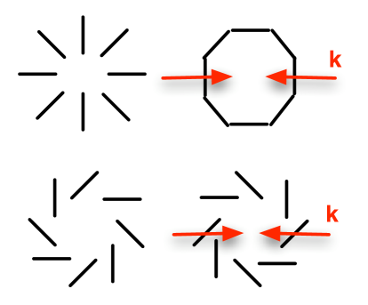
Figure 1: Polarization patterns around an local intensity extremum. The upper row shows the even parity $E$–mode (negative on the left, positive on the right), and the lower row the odd parity $B$–mode (negative on the left, positive on the right). The red arrows illustrate the projected wave vectors of plane wave perturbations converging at the extremum.

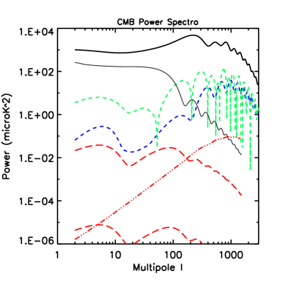
Figure 2: Angular power spectra $l(l+1)C_{l}/2\pi$. The bold solid black line shows the temperature power spectrum of the standard model [5]; the thin black line gives the tensor contribution to the temperature power for $r=0.5$. The green (upper) and blue (lower) short dashed curves are, respectively, the scalar $TE$ (absolute value shown) and $EE$ power spectra for the standard model; the former is well measured on large scales by WMAP [24]. The red long dashed lines indicate the tensor $B$–mode power for $r=0.5$ (upper) and $r=10^{-4}$ (lower). Gravitational lensing produces the $B$–mode power shown as the red 3–dot–dashed curve peaking at $l\sim 1000$.

2.1 Describing CMB Polarization

Polarized light is commonly described with the Stokes parameters [8]. As we have seen, the CMB is linearly polarized, so we use the Stokes parameters $Q$ and $U$, each of which is defined as the intensity difference between two orthogonal polarization directions. Let $(x,y)$ and $(x^{\prime},y^{\prime})$ refer to two coordinate systems situated perpendicular to the light propagation direction and rotated by $45$ degrees with respect to each other. Then $Q\equiv I_{y}-I_{x}$ and $U\equiv I_{y^{\prime}}-I_{x^{\prime}}$.

Clearly, the values of $Q$ and $U$ will depend on the orientation of the coordinate system used at each point on the sky. Although from an experimental viewpoint this is unavoidable, it is better for theoretical purposes to look for a coordinate–free description; this latter could then be translated into any chosen coordinate system. Two such descriptions were first proposed for the CMB by Zaldariagga & Seljak and by Kamionkowski et al. [9]. The former, in particular, model polarization as a spin 2 field on the sphere, an approach used in the publically available CMB codes [10].

The coordinate–free description distinguishes two kinds of polarization pattern on the sky by their different parities. In the spinor approach, the even parity pattern is called the $E$–mode and the odd parity pattern the $B$–mode. We can represent the polarized CMB sky by a map color–coded for intensity and with small bars indicating the direction of linear polarization at each point. Consider a peak in the intensity (see Figure 2). If the polarization bars are oriented either in a tangential or a radial pattern around the peak, we have a $E$–mode; if they are oriented at $45$ degrees (relative to rays emanating from the peak), we have $B$–mode: a reflection of the sky about any line through the peak leaves the $E$–mode unchanged (even parity), while the $B$–mode changes sign (odd parity).

Another useful way to see this is to consider the wave vectors of the plane wave perturbations making up the intensity peak; they radially point towards the peak center (see Figure). We then see that an $E$–mode plane wave has its polarization either perpendicular or parallel to the wave vector. A $B$–mode plane wave, on the other hand, has a linear polarization at $45$ degrees to the wave vector. The wave vector in fact defines a natural coordinate system for definition of the Stokes parameters: in this system, $Q$=$E$ and $U$=$B$. This is particularly useful when discussing interferometric observations.

2.1.1 The $E$–$B$ Decomposition

This decomposition of polarization into $E$ and $B$–modes is powerful and practical. As we shall see below, the two different modes are generated by different physical mechanisms, which is not surprising, since they are distinguished by their parity. Secondly, their different parity also guaranties that we can separate and individually measure the two modes and the total intensity on the sky. This is extremely important because the intensity and polarization anisotropies have very different amplitudes (see Figure 2).

Theory predicts that the primary CMB anisotropy is a Gaussian field (of zero mean), and current observations remain fully consistent with this expectation. We therefore describe CMB anisotropy with the power spectrum $C_{l}$, which is nothing other than the second moment of the field in harmonic space (i.e., the variance). As stated, most of the CMB milestones have been obtained from temperature measurements, which in this context means from measurement of the temperature angular power spectrum $C^{\rm TT}_{l}$. With the introduction of polarization, we see that in fact there are a total of 4 power spectra to determine: $C^{\rm TT},C^{\rm TE},C^{\rm EE},C^{\rm BB}$; parity considerations eliminate the two other possible power spectra, $C^{TB}$ and $C^{EB}$.

2.2 The Physical Content of CMB Polarization

In the standard model, inflation generates both scalar (S), or density perturbations [11] and tensor (T), or gravity wave perturbations [12]. The scalar perturbations are created by quantum fluctuations in the particle field (usually assumed to be a scalar field) driving inflation. After inflation, these perturbations grow by gravity to form galaxies and the observed large scale structure. Gravity waves, on the other hand, decay once they enter the horizon, and thus leave their imprint in the CMB on large angular scales (around and larger than the decoupling horizon, $\sim 1\deg$).

Gravity wave production by inflation, although a reasonable extrapolation of known physics, would nevertheless be something fundamentally new. These waves would not be generated by any classical or even quantum source (i.e., by the right–hand–side of Einstein’s equations); we suppose instead that the gravitational field itself (more specifically, the two independent polarization states of a free gravity wave in flat space) experiences vacuum quantum fluctuations like a scalar field. Finding gravity waves from inflation would therefore not simply be a detection of gravity waves, but also a remarkable observation of the semi–classical behavior of gravity.

Both scalar and tensor perturbations contribute to the temperature power spectrum; in practice, however, the scalar mode dominates, so that the measured temperature spectrum effectively fixes the scalar perturbation amplitude. We quantify the relative amplitude of the scalar and tensor perturbations by the parameter $r\equiv{\cal P}_{\rm T}/{\cal P}_{\rm S}$, where ${\cal P}_{\rm T}$ and ${\cal P}_{\rm S}$ represent the power in the respective modes at a pivot wavenumber [13]. Since the scalar power is measured, we use $r$ to express the gravity wave amplitude. The WMAP data combined with large scale structure data limit $r<0.53$ (95% [14]). Unlike the scalar modes, which depend on the slope of the inflation potential, the gravity wave amplitude depends only on the energy scale of inflation, $E_{\rm I}$ (specifically, ${\cal P}_{\rm T}\propto(E_{\rm I}/M_{\rm pl})^{4}$, where $M_{\rm pl}$ is the Planck mass). Quantitatively, we have $E_{\rm I}=3.4\times 10^{16}$ GeV $r^{1/4}$. Thus, the above limit on $r$ corresponds to an upper limit on the inflation scale of $E_{I}<2.9\times 10^{16}$ GeV.

In addition to these primary CMB polarization signals, gravitational lensing by structures forming along the line–of–sight to the last scattering surface sources a particular kind of secondary polarization signal; I discuss this in the following section.

Figure 2 shows inflationary predictions for the various CMB power spectra from inflation–generated scalar and tensor perturbations. The temperature power spectrum for the standard cosmological model (fit to the WMAP and other higher resolution experimental data) is given by the bold solid black curve. This is now measured to the cosmic variance limit out to the second peak. The light, black solid curve gives the maximum allowable tensor contribution to the temperature power spectrum, i.e., at the current limit of $r<0.53$. Note that it would be very hard to significantly improve on this limit with only temperature measurements. This is why there is such intense interest in polarization.

2.2.1 The Importance of the $E$–$B$ Decomposition

Although both scalar and tensor perturbations generate temperature anisotropy ($C^{\rm TT}$), primordial scalar perturbations only produce $E$–mode polarization, and hence only contribute to $C^{\rm EE}$ and $C^{\rm TE}$. They cannot create $B$–mode polarization. We see this by considering a plane wave scalar perturbation passing over a scattering electron: the local intensity quadrupole around the electron must be aligned with the wave vector, which implies that the polarization of the scattered light must be either perpendicular or parallel to the projected wave vector – in other words, a pure $E$ mode. The axial symmetry imposed by the scalar nature of the density perturbations prevents any $B$–mode production.

The short dashed green (upper) and blue (lower) lines show $C^{\rm TE}$ and $C^{\rm EE}$ power spectra from scalar perturbations for the standard model. These predictions follow directly from the measured temperature power spectrum and the assumption – usually adopted in the standard model – that the scalar perturbations are purely adiabatic. Given the measured temperature spectrum, we could change the predicted $C^{\rm TE}$ and $C^{\rm EE}$ spectra by adding isocurvature perturbations. Observations of these polarization modes will therefore constrain the presence of such isocurvature modes.

The TE cross spectrum in fact changes sign, but since I only plot its absolute value, the curve oscillates between the sharp dips corresponding to the sign change. The additional bump at low multipole arises from reinonization, for which I have taken an optical depth of $\tau=0.17$ [5].

In contrast to scalar perturbations, gravity waves (T) push and pull matter in directions perpendicular to their propagation, aligning the local intensity quadrupole in the plane perpendicular to the wave vector. The loss of axial symmetry allows both $E$ and $B$–mode production. Since the expansion dampens gravity waves on scales smaller than the horizon, these tensor effects only appear on angular scales larger than $\sim 1^{\circ}$ (the angular size of the decoupling horizon). Hence, $B$–mode polarization on large angular scales is the unique signature of primordial gravity waves (the so–called smoking gun) [15].

As mentioned, the amplitude of the gravity wave signal depends only on the energy scale of inflation. A measurement of $B$–mode polarization on large scales would give us this amplitude, and hence a direct determination of the energy scale of inflation.. The red long–dashed curves in Figure 2 show the tensor $B$–mode spectrum for two different amplitudes – the upper curve for the the current limit of $r<0.5$ ($E_{\rm I}\sim 3\times 10^{16}$ GeV), and the lower one for $r=10^{-4}$ ($E_{\rm I}\sim 3.4\times 10^{15}$ GeV).

Gravitational lensing of CMB anisotropy by structures forming along the line–of–sight to decoupling also generates $B$–mode polarization, but on smaller scales [16]. Lensing deviates the photon trajectories (preserving surface brightness) and scrambles (distorts) our view of the decoupling surface [17]. The $E$–$B$ modes are defined as pure parity patterns on the sky; scrambling any such pattern will clearly destroy its pure parity, thereby leaking power into the opposite parity mode. If, for example, there were only $E$–mode perturbations at decoupling (e.g., gravity waves are negligible), we would still see some $B$–mode in our sky maps on small angular scales caused by gravitational lensing.

The lensing signal has both negative and positive aspects in the present context. On the down side, it masks the gravity wave $B$–mode with a foreground signal with an identical electromagnetic spectrum; thus, we cannot remove it using frequency information. We can, however, extract and remove the lensing signal by exploiting the unique mode–mode coupling (between different multipoles, absent in the primary anisotropies) induced by the lensing [18]. Uncertainty in this process may ultimately limit our sensitivity to gravity waves [19].

On the positive side, the lensing signal carries important information about the matter power spectrum and its evolution over a range of redshift inaccessible by any other observation. This provides us with a powerful means of constraining dark energy and a singular method for determining the neutrino mass scale [20]. Since the expansion governs the matter perturbation growth rate, comparison of the amplitude of the power spectrum at high redshift to its amplitude today probes the influence of dark energy. The shape of the power spectrum, on the other hand, is affected by the presence of massive neutrinos, which tend to smooth out perturbations by free streaming out of over– and under–densities. The effect suppresses the power spectrum on small scales.

Recent studies indicate that by measuring the lensing polarization signal to the cosmic variance limit, we would obtain a $1\sigma$ sensitivity to the sum of the 3 neutrino masses of $\sigma_{\Sigma}=0.035$ eV  [20]. This is extremely important: current neutrino oscillation data call for a $\Delta m^{2}=(2.4_{-0.6}^{+0.5})\times 10^{-3}$ eV² ($2\sigma$) [21], implying that the summed mass of the three neutrino species exceeds the ultimate CMB sensitivity. CMB polarization therefore provides a powerful and unique way to measure the neutrino mass scale, down to values unattainable in the laboratory.

The red triple–dot–dashed curve in Figure 2 shows the $B$–mode polarization from lensing. Its amplitude is set by the amplitude of the primordial $E$–mode signal and of the matter power spectrum as it evolves. Since gravity waves generate both $E$–modes (the tensor contribution is not shown in the figure) and $B$–modes of roughly equal power, we expect the scalar $E$–mode to dominate. Thus, we have a good idea of the overall amplitude of the lensing $B$–mode spectrum, although the exact amplitude and shape will depend, as discussed, on the presence of isocurvature modes, neutrinos and the nature of dark energy. For the curve shown in Figure 2, I have adopted the standard model (no isocurvature perturbations) with a pure cosmological constant and have ignored neutrinos.

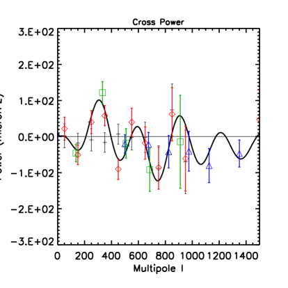
Figure 3: TE power spectra $l(l+1)C_{l}/2\pi$. The curve shows the power predicted by the standard model (and measured on large scales by WMAP [24], although not reproduced here). Red diamonds give the BOOMERanG results, green boxes the DASI 3–year results and blue triangles the CBI results. The thin black error bars show the BOOMERanG $TB$ power, a foreground tracer.

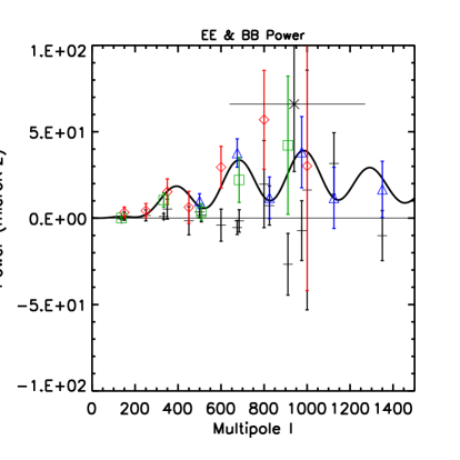
Figure 4: EE and BB power spectra. The curve shows the standard model prediction for $C^{\rm EE}$. Points are labeled as for the previous figure; the black asterisk is the CAPMAP $E$–mode power measurement. Here, the thin black error bars give each experiment’s $B$–mode measurements (all consistent with zero).

3 Observational Effort

We often refer to polarization as the next step in CMB science. While appropriate, this erroneously gives the impression that it remains for the future, when in fact, different experiments have already measured CMB polarization. I give a summary in Figures 4 and 4.

The DASI experiment at the South Pole was the first to detect CMB polarization, both $E$ and $TE$ modes [22]; their recently published 3–year results [23] are shown in Figures 4 and 4 as the green squares. The original DASI detection was followed by WMAP’s measurement of $C^{\rm TE}$ on large scales down to $l\sim 500$ from the first year data [24]; these are not reproduced here.

More recently, the BOOMERanG collaboration reports measurements of $C^{\rm TT}$, $C^{\rm TE}$ and $C^{\rm EE}$ and a non–detection of $B$–modes [25]. Combining their new BOOMERanG data with other CMB and large scale structure data, MacTavish et al. [26] constrain $r<0.36$ (95%). These results are shown in Figures 4 and 4 as the red diamonds.

The CBI experiment has also published new measurements of $C^{\rm TT}$, $C^{\rm TE}$ and $C^{\rm EE}$, as well as a non–detection of $B$– modes [27]. These are shown in Figures 4 and 4 as the blue triangles. Finally, the black asterisk in Figure 4 gives the $E$–mode power measurement by CAPMAP [28]. All of these results are consistent with each other and with the prediction of the standard cosmological model assuming pure adiabatic modes, shown in the figures as the black curve.

Although these new $B$–mode limits are still far from placing any important constraints on either gravity waves or lensing, the results are significant for what they imply about Galactic foregrounds. We expect these foregrounds to generate $E$– and $B$–modes with equal strength – there is no symmetry preferring one over the other. The lack of $B$–mode power thus suggests that foreground contamination in these data sets is well below the measured $E$ and $TE$ signals.

Scheduled for launch in 2007/2008, the Planck satellite will greatly advance our knowledge of CMB polarization by providing foreground/cosmic variance–limited measurements of $C^{\rm TE}$ and $C^{\rm EE}$ out beyond $l\sim 1000$. We also expect to detect the lensing signal, although with relatively low precision, and could see gravity waves at a level of $r\sim 0.1$. The Planck blue book quantifies these expectations.

A leap in instrument sensitivity is required in order to go beyond Planck and get at the $B$–modes from lensing and gravity waves. This important science is motivating a vast effort world wide at developing a new generation of instruments based on large detector arrays. Numerous ground–based and ballon–borne experiments are actually observing or being prepared. In the longer term future, both NASA (Beyond Einstein) and ESA (Cosmic Vision) have listed a dedicated CMB polarization mission as a priority in the time frame 2015-2020. Such a mission could reach the cosmic variance limit on the lensing power spectrum to measure the neutrino mass scale and perhaps detect primordial gravity waves from inflation near the GUT scale. The exciting journey has begun.

References

References

- [1] Smoot G F et al. 1992 ApJ 396 L1 \nonumLange A E et al. 2001 Phy. Rev. D 63 042001 \nonumStompor R et al. 2001 ApJ 561 L7 \nonumBennett C L et al. 2003 ApJS 148 1 \nonumScott D and Smoot G 2006 The Review of Particle Physics (Preprint astro–ph/0601307)
- [2] Knop R A et al. 2003 ApJ 598 102 \nonumRiess A G et al. 2004 ApJ 607 665 \nonumAstier P et al. 2005 Preprint astro–ph/0510447
- [3] Freedman W L et al. 2001 ApJ 553 47
- [4] Tegmark M et al. 2004 ApJ 606 702 \nonumCole S et al. 2005 MNRAS 362 505
- [5] Spergel D N et al. 2003 ApJS 148 175 \nonumSeljak U et al. 2005 Phys. Rev D 71 103515 \nonumSanchez A G et al. MNRAS in press (Preprint astro–ph/0507583)
- [6] Steigman G 2005, Preprint astro–ph/0511534
- [7] Bond J R and Efstathiou G 1984 ApJ 285 L45 \nonumHu W and White M 1997 New Astron. 2 323
- [8] Rybicki G B and Lightman A P 1979 Radiative processes in astrophysics (New York: Wiley–Interscience)
- [9] Zaldarriaga M. and Seljak U 1997 Phys. Rev. D 55 1830 \nonumKamionkowski A, Kosowsky A and Stebbins A 1997 Phys. Rev. D 55 7368
- [10] Seljak U and Zaldarriaga M 1996 ApJ 469 437 (http://www.cmbfast.org) \nonumLewis A, Challinor A and Lasenby A 2000 ApJ 538 473 (http://camb.info)
- [11] Mukhanov V F and Chibisov G V 1981 JETP Lett. 33 532 \nonumGuth A H and Pi S–Y 1982 Phys. Rev. Lett 49 1110 \nonumHawking S W 1982 Phys. Lett. B 115 295 \nonumStarobinsky A A 1982 Phys. Lett. B 117 175 \nonumBardeen J M, Steinhardt P J and Turner M S 1983 Phys. Rev. D 28 679
- [12] Starobinsky A A 1979 JETP Lett. 30 682 \nonumVeryaskin A V, Rubakov V A and Sazhin M V 1983 Soviet Astron. 27 16 \nonumAbbott L F and Wise M 1984 Nucl. Phys. B 244 541 \nonumKamionkowski M and Kosowsky A 1999 Ann. Rev. Nucl. Part. Sci. 49 77
- [13] Leach S M, Liddle A R, Martin J and Schwarz D J 2002 Phys. Rev. D 66 023515
- [14] Peiris H V et al. 2003 ApJS 148 213
- [15] Seljak U and Zaldarriaga M 1997 Phys. Rev. Lett. 78 2054 \nonumKamionkowski M, Kosowsky A and Stebbins A 1997 Phys. Rev. Lett. 78 2058
- [16] Zaldarriaga M and Seljak U 1998 Phys. Rev. D 58 023003
- [17] Blanchard A and Schneider J 1987 A&A 184 1 \nonumSeljak U 1996 ApJ 463 1 \nonumBernardeau F 1997 A&A 324 15
- [18] Hu W and Okamoto T 2002 ApJ 574 566 \nonumOkamoto T and Hu W 2003 Phys. Rev. D 67 083002
- [19] Knox L and Song Y-S 2002 Phys. Rev. Lett. 89 011303 \nonumKesden M, Cooray A and Kamionkowski M 2002 Phys. Rev. Lett. 89 011304 \nonumSeljak U and Hirata C M 2004 Phys. Rev. D 69 043005
- [20] Kaplinghat M, Lloyd K and Song Y–S 2003 Phys. Rev. Lett. 91 241301 \nonumKaplinghat M 2003 New. Astron. Rev. 47 893 \nonumLesgourgues J, Perotto L, Pastor S and Piat M 2005 Preprint astro–ph/0511735
- [21] Fogli G L, Lisi E, Marrone A and Palazzo A 2005 Preprint hep–ph/0506083
- [22] Kovac J M, Leitch E M, Pryke C, Carlstrom J E, Halverson N W and Holzapfel W L 2002 Nature 420 772
- [23] Leitch E M, Kovac J M, Halverson N W, Carlstrom J E, Pryke C and Smith M W E 2005 ApJ 624 10
- [24] Kogut et al. 2003 ApJS 148 161
- [25] Piacentini F et al. 2005 Preprint astro–ph/0507507 \nonumMontroy T E et al. 2005 Preprint astro–ph/0507514
- [26] MacTavish C J et al. 2005 Preprint astro–ph/0507503
- [27] Sievers J L et al. 2005 Preprint astro–ph/0509203
- [28] Barkats D et al. 2005 ApJ 619 L127