First Results from IceCube

Abstract

IceCube is a 1 km³ neutrino observatory being built to study neutrino production in active galactic nuclei, gamma-ray bursts, supernova remnants, and a host of other astrophysical sources. High-energy neutrinos may signal the sources of ultra-high energy cosmic rays. IceCube will also study many particle-physics topics: searches for WIMP annihilation in the Earth or the Sun, and for signatures of supersymmetry in neutrino interactions, studies of neutrino properties, including searches for extra dimensions, and searches for exotica such as magnetic monopoles or Q-balls. IceCube will also study the cosmic-ray composition.

In January, 2005, 60 digital optical modules (DOMs) were deployed in the South Polar ice at depths ranging from 1450 to 2450 meters, and 8 ice-tanks, each containing 2 DOMs were deployed as part of a surface air-shower array. All 76 DOMs are collecting high-quality data. After discussing the IceCube physics program and hardware, I will present some initial results with the first DOMs.

1 IceCube Physics Program

Neutrinos are strongly penetrating particles that can be used to search for the sources of high-energy cosmic rays and study many energetic astrophysical phenomena. Except at the very highest energies (above 50 EeV), high-energy protons and nuclei are bent in the interstellar magnetic fields, and high-energy photons are absorbed by interactions with the $3^{0}$K microwave background and infrared photons from red-shifted starlight. Only neutrinos can provide a clear view of the sky above 50 TeV. The primary purpose of IceCube is to map out this sky PDD ; many calculations using a wide variety of approaches find that a volume of at least 1 km³ detector is required to observe neutrino sources icsense . Neutrinos are expected as ‘by-products’ of hadronic acceleration, and may be observed from active galactic nuclei (AGNs), gamma-ray bursters (GRBs), and possibly supernova remnants.

The completed IceCube detector will collect data on about 100,000 atmospheric $\nu$/year atmosphere . These neutrinos can be used to measure the neutrino-nucleon cross sections (through absorption in the earth) and search for new forms of neutrino oscillations, such as those predicted by some models of quantum gravity qg ).

IceCube will also search for signs of supersymmetry (some parameter sets with high mass scales lead to pairs of upward going particles in the detector) SUSY , neutrinos from WIMP annihilation in the Earth or the Sun WIMPs , and for exotic particles like magnetic monopoles, Q-balls, and the like. IceCube also serves as a supernova monitor; a supernova in our galaxy should increase the singles rates of all of the in-ice phototubes supernova .

2 Hardware overview

IceCube is building on the experience of AMANDA, which studied a variety of neutrino topics paolo . IceCube will instrument 1 km³ using 4800 digital optical modules (DOMs). The DOMs will be deployed in 80 strings on a 125 meter hexagonal grid. Each string will contain 60 modules at a 17 meter spacing.

Each DOM acts like a mini-satellite, acquiring data autonomously. A DOM consists of a 13” pressure vessel (Benthosphere) containing a Hamamatsu R7081-02 10” photomultiplier tube (PMT), PMT base, flasher (LED) board and a main electronics board. The main board, Fig. 1, includes front-end electronics and trigger, two analog-to-digital converter systems, a precision clock and a large field programmable gate array (FPGA), with an integrated CPU, for control, communications, etc stokstad . All communication with the surface is through a single twisted-wire pair (shared by 2 DOMs); this single pair carries power, bi-directional data, and timing calibration signals.

The PMT gains are currently set at $10^{7}$. The PMT signal is AC coupled through a transformer on the base. The signal is fed to a discriminator and two separate digitizer circuits. The discriminator is typically set at about 1/3 of a photoelectron pulse. When the discriminator fires, a digitization cycle begins on the next clock transition.

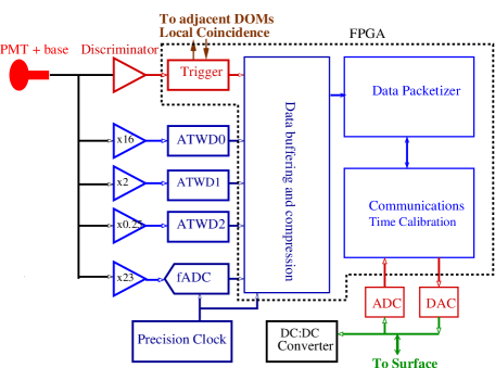
Figure 1: A block diagram of an IceCube DOM main board.

The first digitizer is based on a custom switched-capacitor-array chip, the Analog Transient Waveform Digitizer (ATWD). It takes 128 samples at from 200 to 700 megasamples per second (MSPS), and then digitizes them with 10-bit resolution. IceCube is currently running at 300 MSPS. The PMT signal feeds 3 ATWD channels, with a nominal gain ratio of 0.25:2:16; combined, the three channels offer 14 bits of resolution, covering from single photoelectrons up to the maximum PMT voltage. To reduce dead time, each DOM contains two ATWDs which operate in a ping-pong fashion. A precision 20 MHz clock is a local reference, used to relate the ATWD launch time to global time.

The other digitizer system detects late arriving light which has scattered in the ice. It uses a 10-bit 40-MSPS commercial ADC to record signals arriving up to 6.4$\mu$s after the DOM launch. The ADC input signals are shaped to ensure that single photoelectrons are observable.

A local coincidence circuit can select which data is transmitted to the surface. Adjacent DOMs are connected by cables, and DOMs can be configured to react differently to events where adjacent (or next-to-nearest neighbor) DOMs are also hit.

The DOMs FPGA controls the data acquisition and storage, compresses the data, packetizes it, and transmits the packets to the surface. It controls and calibrates the system, monitors temperatures and voltages, and monitors the discriminator singles rate; the latter also serves as a monitor to search for supernovae. The DOM communicates with the surface via analog-to-digital and digital-to-analog converters connected to the twisted pairs.

The DOM clock is a precision 20 MHz oscillator, with a short-term frequency stability (Allen variance) of $\delta\!f\!/\!f<10^{-10}$. To maintain accurate inter-DOM timing, the clocks are periodically (currently once every 2.5-3.5 seconds) calibrated by a process known as reciprocal active calibration (RapCal). A pulse is sent from the surface down to the DOM. The signal is received, held for a specified time, and then retransmitted to the surface. By using identical DACs and ADCs at both the DOM and the surface, the transmission time will be the same in both directions; by comparing the surface and DOM clocks, an accurate calibration can be maintained. Data (discussed below) show that the system maintains timing across the entire array to better than 2 nsec, considerably below the design requirement of 5 nsec chirkin .

The DOM “flasher boards” hold 12 light emitting diodes (LEDs) spaced around the DOM. Half of the LEDs point horizontally outward, while the other half point upwards at $45^{o}$. These LEDs are used for calibration, and can mimic $\nu_{e}$ induced showers. The LEDs are individually switchable, and the overall pulse width and amplitude and programmable.

On the surface, the DOM cables are connected to Digital Receiver cards, which plug into PCI slots in off-the-shelf computers. $\pm$ 48 volt power supplies power the DOMs through the DOR card. A software trigger uses data from all of the DOMs to select interesting time regions (events) for storage to disk and/or satellite transmission to the North. The basic algorithm uses the hit multiplicity in a specified time window; future algorithms may also examine the topology and launch times of the hit DOMs. A GPS clock provides absolute timing information.

The IceTop surface air-shower array will consist of 160 tanks, two near the top of each in-ice string. Each consists of 2 DOMs frozen into a 2.7 m diameter ice-filled tank. The tanks are sensitive to both muons and electromagnetic particles (electrons and photons) in cosmic-ray air showers. IceTop will be used as an air-shower array, as a calibration aid for the in-ice array, and as a veto for IceCube. By using the in-ice detectors as a veto, it may also be used to search for high energy gamma rays. As an air-shower array, the system will have a threshold of about 320 TeV.

3 The 2004/2005 deployment

IceCube deployment began with the assembly of the hot water drill in Dec. 2004. A 5-megawatt heater pumps 750 liters/minute of water to the drill head; during 2004/5, the drill reached speeds of about 1 meter/minute; the complete hole drilling (including going through the ‘firn’ region of packed snow), took about 50 hours; in 2005/6 this time is being reduced significantly.

The first IceCube string was deployed in about 16 hours on Jan. 18, 2005. After deployment, it took a few days for the water around most of the DOMs to freeze. For the deepest DOMs, temperatures are higher, so freeze-in required a few weeks.

Logistics are a critical issue for IceCube. The ‘summer’ season (the only time transportation is available, and when active work is possible) runs from late October until February 14th. Even then, construction is heavily constrained by airlift capacity; everything from people to fuel must fit on ski-equipped LC-130 turboprops.

4 Results from the first string

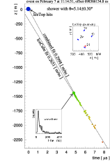
Figure 2: (left) An event that triggered both the IceTop and in-ice subdetectors. For the in-ice detectors, the colors indicate the time that the DOM fired, from green to yellow. One inset shows on an ATWD waveform from one of the DOMs; the other shows the IceTop geometry. The two fits are with and without the IceTop data. (right) The inverse scattering distance for light (averaged over the IceCube spectral range) as a function of depth.

Most of the results to-date have been obtained studying cosmic-ray muons and using the flasher boards. Figure 2 shows an event that triggered both the in-ice and IceTop detectors. The four circles at the top of the picture show the IceTop stations. The air shower was reconstructed using a plane wave fit to the IceTop stations; the in-ice muon was reconstructed with a maximum likelihood fit that accounted for the depth-dependent scattering of the Cherenkov photons in the ice. Figure 2 (right) shows the inverse scattering distances used. Because only a single string is present, the azimuthal angle of the muon cannot be determined.

The left panel of Figure 3 shows the number of hit DOMs in reconstructed muon tracks, while the right panel shows the zenith angle distribution for reconstructed muons of different minimum multiplicities, compared with simulations. The Monte Carlo used here did not include simulate the ATWD waveforms, so some deviation is to be expected.

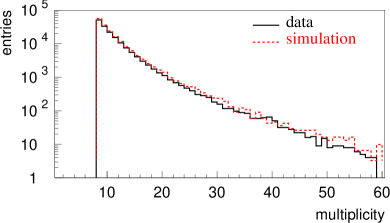
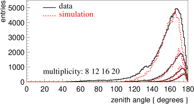
Figure 3: (left) The number of hit DOMs in muon tracks, compared with simulation. At least 8 hits are required for a trigger. (right) The zenith angle distribution for muons events with multiplicity at least 8, 12, 16 or 20 hits, compared with the corresponding simulations. Here 180⁰ points straight downward.

Muon tracks are used to verify the detector time resolution. The muon track is fit with a given DOM excluded, and then the residual to that DOM is histogrammed. Figure 4 (left) shows these residuals for a DOM; the long asymmetric tail is due to light scattering in the ice, which delays the photons. The effect of scattering is minimized by using only muon tracks which pass close to the DOM whose timing is being measured. Fig. 4 (right) shows the mean residuals when this procedure is applied to all 60 DOMs. As Fig. 2 (right) shows, DOMs 35-45 are in particularly dusty ice, with a short scattering length; this scattering causes the means to rise above 0. Still, these muon fits show that the DOM timing is correct to within 3 nsec.

Figure 4: (left) The distribution of timing residuals for a muon track. Time 0 corresponds to that expected for direct light from the track; most of the width of the peak comes from errors in the fit, particularly the distance from the muon to the DOM. (right) The mean of the distributions of residuals for all 60 DOMs.

The flasher-board LEDs are also used to study detector performance. Figure 5 (center) shows the measured time difference between DOMs 45 and 46 when DOM 47 is flashing (as shown at the far left of Fig. 5); the sigma of the distribution is 1.26 nsec. The left histogram shows the measured time differences for the 58 adjacent DOM pairs; all the pairs have sigmas under 2 nsec.

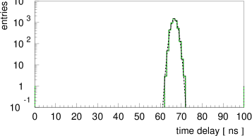
Figure 5: (left) DOM 47 is flashing. (center) The first photon arrival time difference between DOMs 45 and 46. (right) The arrival time differences for the 58 pairs of adjacent DOMs above a flashing DOM.

5 Conclusions

In 2004/5 the IceCube collaboration deployed a string of 60 DOMs at the South Pole, along with 8 ice-tanks containing an additional 16 DOMs. All 76 DOMs are working well, and the system shows time resolutions of $\approx 2$ nsec. In 2005/6, we expect to deploy an additional 8-12 strings, moving toward completion of the 80-string array by 2010.

References

- (1) The IceCube Collaboration, Preliminary Design Document, 2001. Available from http://icecube.wisc.edu/pub_and_doc/.
- (2) J. Ahrens et al., Astropart. Phys. 20, 507 (2004).
- (3) M. C. Gonzalez-Garcia, F. Halzen and M. Maltoni, Phys. Rev. D71, 093010 (2005).
- (4) L. Anchiordoqui et al., Phys. Rev. D72, 065019 (2005).
- (5) I. F. Albuquerque, G. Burdman and Z. Chako, Phys. Rev. Lett. 92, 221802 (2004).
- (6) I. F. Albuquerque, J. Lamoreaux and G. Smoot, Phys. Rev. D66, 125006 (2002).
- (7) A. S. Dighe et al., JCAP 0306, 005 (2003).
- (8) P. Desiati, these proceedings.
- (9) R.G. Stokstad, for the IceCube Collaboration, presented at 11th Wkshp on Electronics for LHC and Future Experiments, Sept. 12-16, 2005, Heidelberg, Germany.
- (10) D. Chirkin, in astro-ph/0509330.