The Two Young Star Disks in the Central Parsec of the Galaxy: Properties, Dynamics and Formation

Abstract

We report the definite spectroscopic identification of $\simeq 40$ OB supergiants, giants and main sequence stars in the central parsec of the Galaxy. Detection of their absorption lines have become possible with the high spatial and spectral resolution and sensitivity of the adaptive optics integral field spectrometer SPIFFI/SINFONI on the ESO VLT. Several of these OB stars appear to be helium and nitrogen rich. Almost all of the $\simeq 80$ massive stars now known in the central parsec (central arcsecond excluded) reside in one of two somewhat thick ($\langle|h|/R\rangle\simeq 0.14$) rotating disks. These stellar disks have fairly sharp inner edges ($R\simeq 1\arcsec$) and surface density profiles that scale as $R^{-2}$. We do not detect any OB stars outside the central $0.5$ pc. The majority of the stars in the clockwise system appear to be on almost circular orbits, whereas most of those in the ‘counter-clockwise’ disk appear to be on eccentric orbits. Based on its stellar surface density distribution and dynamics we propose that IRS 13E is an extremely dense cluster ($\rho_{\mathrm{core}}\gtrsim 3\times 10^{8}M_{\sun}$ pc^-3), which has formed in the counter-clockwise disk. The stellar contents of both systems are remarkably similar, indicating a common age of $\simeq 6\pm 2$ Myr. The K-band luminosity function of the massive stars suggests a top-heavy mass function and limits the total stellar mass contained in both disks to $\simeq 1.5\times 10^{4}M_{\sun}$. Our data strongly favor in situ star formation from dense gas accretion disks for the two stellar disks. This conclusion is very clear for the clockwise disk and highly plausible for the counter-clockwise system.

1 INTRODUCTION

The Galactic Center (GC) is a unique laboratory for studying galactic nuclei. Given its proximity, processes in the GC can be investigated at resolutions and detail that are not accessible in any other galactic nucleus (unless otherwise specified we adopt a distance of 8 kpc for simplicity of comparison to earlier work; we specifically use the most recent value $R_{0}=7.62\pm 0.32$ kpc by Eisenhauer et al. 2005 when the $\simeq 5\%$ error could lead to a significant bias). The GC has many features that are thought to occur in other nuclei (for reviews, see Genzel & Townes 1987; Morris & Serabyn 1996; Mezger, Duschl & Zylka 1996; Alexander 2005). It contains the densest star cluster in the Milky Way intermixed with a bright H II region (Sgr A West or the ‘mini-spiral’) and hot gas radiating at X-rays. These central components are surrounded by a $\simeq 1.5$ pc ring/torus of dense molecular gas (the ‘circum-nuclear disk’, CND). At the very center lies a very compact radio source, Sgr A*. The short orbital period of stars (in particular the B star S2) in the central arcsecond around Sgr A* show that the radio source is a $3$–$4\times 10^{6}M_{\sun}$ black hole (BH) beyond any reasonable doubt (Schödel et al. 2002; Ghez et al. 2003). The larger Galactic Center region contains three remarkably rich clusters of young, high mass stars: the Quintuplet, the Arches, as well as the parsec-scale cluster around Sgr A* itself (Figer 2003).

In seeing-limited near-infrared images of the central region of the Galactic Center, several bright sources dominate the $\simeq 20\arcsec\times 20\arcsec$ field centered on Sgr A*. Among these, the IRS 16 cluster (Becklin & Neugebauer 1975) is a bright source of broad He I 2.058 µm line emission (Hall, Kleinmann & Scoville 1982). IRS 16 has been since then resolved into a cluster of about a half a dozen stars (Forrest et al. 1987, Allen, Hyland & Hillier 1990, Krabbe et al. 1991, 1995, Tamblyn et al. 1996, Paumard et al. 2001). These appear to be post main-sequence OB stars in a transitional phase of high mass loss (Morris et al. 1996), between extreme O supergiants and Wolf-Rayet (WR) stars (Allen et al. 1990; Najarro et al. 1994, 1997; Trippe et al. 2005). They have been classified as Ofpe/WN9 stars (Allen, Hyland, & Hillier 1990) and have been suggested as Nitrogen-rich OB stars (OBN) stars by Hanson et al. (1996) and as Luminous Blue Variables (LBV) candidates by Paumard et al. (2001). There is no a-priori incompability between these tentative classifications that are based on different properties. Several dozens of even more evolved WR stars have been observed in the same region (e.g. Krabbe et al. 1995; Blum, Sellgren & DePoy 1995; Paumard et al. 2001). The lack of OB stars in these earlier studies is puzzling. The question is whether this lack is due to a true depletion or is merely a selection effect due to veiling of the weak absorption lines in near main sequence stars by bright nebular emission. Adaptive optics (AO) spectroscopy of the center-most arcsecond around Sgr A* (mostly devoid of nebular emission) has already revealed a dozen massive stars. These stars appear to be main sequence late O and B stars and orbit the central black mass at distances as short as a few light-days (Schödel et al. 2003; Ghez et al. 2003, 2005; Eisenhauer et al. 2005).

These observations show that massive star formation has occurred at or near the Galactic Center within the last few million years. This is surprising. All obvious routes to creating or bringing massive young stars in(to) the central region face major obstacles. In situ star formation, transport of stars from far out, scattering of stars on highly elliptical orbits and rejuvenation of old stars due to stellar collisions and tidal stripping have all been proposed and considered (for a recent review of the rapidly growing body of literature see Alexander 2005). No explanation at this point is the obvious winner (or loser). Perhaps the two most prominent and promising scenarios for explaining the young massive stars outside the central cusp, at radii of 3–$10\arcsec$ from Sgr A*, are

1. the ‘in situ, accretion disk’ scenario (Levin & Beloborodov 2003; Genzel et al. 2003; Goodman 2003; Milosavljevic & Loeb 2004; Nayakshin & Cuadra 2005). Here the proposal is that stars have formed near where they are found today, very close to the central black hole. However, in situ star formation is impeded by the tidal shear from the central black hole and surrounding dense star cluster. To overcome this shear, gas clouds have to be much denser ($\simeq 10^{12}R_{1\arcsec}^{-3}$ cm^-3) than currently observed (Morris 1993). The tidal shear can be overcome if the mass accretion was large enough at some point in the past – perhaps as the consequence of the in-fall and cooling of a large interstellar cloud – such that a gravitationally unstable (outside of a critical radius) disk was formed. The stars were formed directly out of the fragmenting disk;

2. the ‘in-spiraling star cluster’ scenario (Gerhard 2001; McMillan & Portegies Zwart 2003; PortegiesZwart et al. 2003; Kim & Morris 2003; Kim, Figer, & Morris 2004; Gürkan & Rasio 2005). Here the idea is that young stars were originally formed outside the hostile central parsec and only transported there later on. Individual transport of stars by two body relaxation and mass segregation from further out takes too long a time ($\simeq 10^{7.5}$–$10^{9}$ years: Alexander 2005). Stars in a bound, massive cluster can sink in much more rapidly owing to dynamical friction (Gerhard 2001). To sink from an initial radius of a few parsec or more to a final radius of $\ll 1$ pc within an O star lifetime (a few Myr) requires a cluster mass $>10^{5}M_{\sun}$. To prevent the final tidal disruption of such a cluster at too large a radius – resulting in the deposition of its stars there – the core of the original star cluster also has to be much denser ($>10^{7}M_{\sun}$ pc^-3) and more compact ($\ll 1$ pc) than any known cluster. However, as a helpful by-product, dynamical processes in such a hypothetical super-dense star cluster may then lead to the formation of a central, intermediate mass black hole (IMBH; Portegies-Zwart & McMillian 2002; Gürkan et al, 2004). Such a black hole may help to stabilize the cluster core against tidal disruption and lessen the high density requirement somewhat (Hansen & Milosavljevic 2003).

The ‘paradox of youth’ in the central S-star cluster, with $>15$ apparently normal main sequence B stars residing in tightly bound orbits in the central light month around the central black hole, probably requires yet another explanation (recently Ghez et al. 2003, 2005; Genzel et al. 2003; Hansen & Milosavljevic 2003; Gould & Quillen 2003; Alexander & Livio 2004; Eisenhauer et al. 2005; Alexander 2005; Davies & King 2005). Perhaps the most promising route to get the B stars into the central arcsecond is a scattering process from the reservoir of massive, young stars at $\simeq 3$–$10\arcsec$ (e.g. Alexander & Livio 2004).

To test these proposals, the detailed properties and dynamics of the massive stars in the central parsec must be studied. These properties include exact stellar type, spatial distribution and 3D space velocities. For this purpose, high-resolution imaging and spectro-imaging are required. The new adaptive optics assisted, near-infrared integral field spectrometer on the ESO-VLT, SPIFFI/SINFONI (Eisenhauer et al. 2003b; Bonnet et al. 2004) represents a key new capability for addressing the issues discussed above. We report in this paper SPIFFI/SINFONI observations in 2003, 2004 and 2005 that give important new information on the location, dynamics and evolution of the massive, early type stars in the central parsec. We begin by discussing the SPIFFI/SINFONI observations and data analysis in Sect. 2. This is followed by presentation of our results in Sect. 3. In Sect. 4 we discuss the implications of our findings. Further technical details are presented in the Appendices.

2 OBSERVATIONS AND DATA ANALYSIS

2.1 Observations

SPIFFI (Eisenhauer et al. 2003b,c) is a near-infrared integral field spectrometer providing a 2048 pixel spectrum simultaneously for a contiguous, $64\times 32$-pixel field. Its salient features include a reflective image slicer and a grating spectrometer with an overall detective throughput (including pre-optics module and telescope) of $\geq 30\%$. Its $2048^{2}$-pixel Hawaii II detector covers the J, H and K (1.1 to 2.45 µm) atmospheric bands. In its 2003 version with a smaller $1024^{2}$-pixel detector the spectrometer provided 1024 spectra for a $32^{2}$-pixel field. Spectral resolving powers range from $R=1000$ to 4000. Three pixel scales ($12.5\times 25$ square milli-arcseconds (mas), $50\times 100$ mas² and $125\times 250$ mas²) can be chosen on the fly. In the SINFONI ESO VLT facility, SPIFFI is mated with the MACAO adaptive optics module (Bonnet et al. 2003) employing a 60-element wave-front-curvature sensor with avalanche photodiodes. This mode makes it possible to perform spectroscopy at the smallest (diffraction limited) pixel scale.

Table 1: Summary of SPIFFI/SINFONI Data Sets

Date	Band	Pixel	2D res.	Mosaic size	Comments
		mas	mas	arcsec$\times$arcsec
2003 Apr 8–9	K	100	250	$10\times 10$	Excellent seeing
2003 Apr 8–9	H+K	250	900	$38\times 32$	$\cdots$
2004 Aug 18–19	K	100	220	$10\times 10$	$\cdots$
2005 Mar 14–23	K	100	200	$6\times 16$	Centered $\simeq 15\arcsec$ N of Sgr A*; very deep spectroscopy ($m_{K\mathrm{,lim}}\simeq 16$–17.5)
2005 Mar 14–23	K	100	200	$4\times 20$	Long dimension SW–NE; centered $\simeq 15\arcsec$ NE of Sgr A*
2005 Jun 17	K	250	1000	$40\times 40$	‘Frame’ completing 2003 H+K mosaic

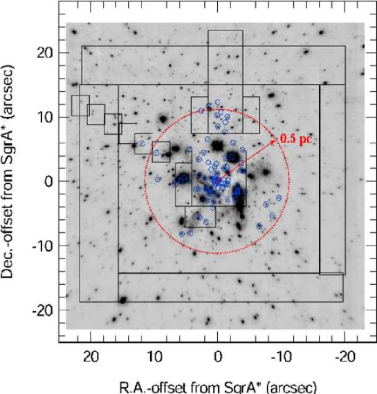
Figure 1: Outline of the various 2003–2005 SPIFFI/SINFONI H+K and K-band cubes (outlines), superposed on a $\simeq 100$ mas resolution, L-band NACO image (logarithmic scale). Small circles denote the 90 quality 1 and 2 early type stars (OB I–V, Ofpe/WN9, WR-stars) reported in this paper (Table 2). A dotted circle denotes a 0.5 pc radius zone centered on Sgr A*, within which essentially all OB stars we have found appear to lie.

Table 1 lists the various data sets we have been able to obtain with both SPIFFI as a guest instrument (in 2003) and SINFONI during its commissioning in 2004 and guaranteed time observation (GTO) runs in 2005. These data have been taken in the K-band with a resolution $R=4000$ (full width at half maximum $\mathrm{FWHM}=85$ km s^-1) and in the H+K mode ($R=1500$, $\mathrm{FWHM}=230$ km s^-1). Preliminary results from the 2003 seeing limited datasets were presented in Genzel et al. (2003), Horrobin et al. (2004) and Paumard et al. (2004a). The 2004 mosaic supersedes the 2003 K-band one. Although the FWHM resolution of these two sets is almost identical, the AO reduced dramatically the wings of the point spread function (PSF), rending unnecessary the complex method for correction of the nebular emission described in Paumard et al. (2004a). Figure 1 shows the coverage of these spectral cubes, superposed on a diffraction limited L^′-band (3.76 µm) image taken with NACO.

We also analyzed several high-quality H- and K_s-band, diffraction limited images taken during 2002–2004 with NACO during our GTO astrometry imaging program to construct very deep images of the IRS 13E and IRS 16 regions. We will return to this when we discuss these images in Sect. 3.3.

2.2 Spectral Identification of Early Type Stars

Interpretation of stellar spectra in the Galactic Center is hindered by stellar crowding and ionized interstellar gas emission, especially in H I $\lambda$ 2.166 µm (Br$\gamma$) and He I $\lambda$ 2.058 µm. As a result, previous seeing limited spectroscopic observations have relatively easily detected broad emission line stars, such as WR stars and other evolved objects (Ofpe/WN stars), but have not been successful in detecting near main-sequence OB stars. These are characterized by relatively weak, absorption features of He I ($\lambda$ 2.058, 2.113, 2.163 µm) and H I Br$\gamma$ (Hanson et al. 2005; the feature at 2.113 µm is in fact a compound of 4 He I lines and three N III lines). The new high-resolution SINFONI data overcome both of these issues to a considerable extent. We can now reliably detect all OB supergiants and giants ($m_{K}\simeq 11$–13). In less crowded regions without strong nebular emission we are now also successful in detecting OB main sequence stars ($m_{K}\simeq 13$–15; see also Eisenhauer et al. 2005).

We searched for OB stars by visual inspection of 2D continuum-subtracted line maps in the above-mentioned lines. Br$\gamma$ and He I $\lambda$ 2.058 µm are usually intrinsically stronger than He I $\lambda$ 2.113 µm, but the latter does not suffer from the problem of nebular emission. This line is, therefore, a good choice for identification of OB stars, especially in the lower resolution H+K data. The spectra of the OB candidates so identified were then extracted with the interstellar emission removed by subtracting an off-source spectrum (generally from a ring around each source).

For the medium plate scale ($50\times 100$ mas²/pixel) K band data, the diffuse emission can in most cases be successfully removed by this subtraction. The correction is not perfect, especially for stars embedded in the interstellar medium, which they excite locally. In other cases the profiles of the interstellar emission are complex and vary rapidly from position to position (Paumard et al. 2004b). As a result there remain considerable uncertainties around Br$\gamma$ and He I $\lambda$ 2.058 µm in the spectra extracted near/on mini-spiral streamers. In a few cases, especially for fainter stars, the spectral identification of the stars is not certain. We have taken these issues into account by grouping stars into three quality codes. Stars with code 2 have high quality spectra and certain identification. Stars with code 1 have possible uncertainties in the extraction of some of the key spectral features. In the case of stars with code 0 the identification (as early type stars) is preliminary and needs to be confirmed. For a positive identification of a candidate Br$\gamma$ absorption line star we require that the stellar spectrum does not exhibit any signs for the 2.3–2.4 µm CO overtone absorption bands characteristic of late type stars.

In the larger K and H+K cubes at lower spectral and spatial resolution (the outer square and rectangles in Fig. 1), the nebular emission subtraction becomes much harder. There remains only the possibility of looking for the He I/N III complex at 2.113 µm as explained above but the cube in this case is filled with an unresolved background of late-type stars: the CO break at 2.29 µm, which is obvious in almost every pixel in the field, cannot be used as a discriminator. All spectra are contaminated to some extent by the numerous absorption lines that the cool stars exhibit (Wallace & Hinkle 1997 speak of a “grass” of absorption lines). We see in particular Al I ${\lambda}$ 2.1099, 2.1132 and 2.1170 µm. This makes the identification of He I ${\lambda}$ 2.1127 µm uncertain or even doubtful. While we find many emission line stars in this cube, we regard the identification of a number of absorption line stars as reasonably safe, and classify them with the same quality codes.

To obtain stellar identifications we compared the extracted spectra with templates from the literature. For the wind-dominated stars and WR stars we mainly used the atlas of Morris et al. (1996) and Figer, McLean & Najarro (1997). For the OB stars we referred to Hanson et al. (1996, 2005). We compared spectra from the latter atlas individually to the Galactic Center stars and made spectral identifications based on the strength of the He I, H I, He II, and N III lines, along with equivalent widths and line profiles/widths. We computed absolute magnitudes from the observed magnitudes and individual extinction corrections (Appendix F). These absolute K magnitudes are used in our final classifications (Table 2) as an additional constraint for placing the stars in the different luminosity classes.

Table 2: Properties of Early Type Stars (Quality 1+ 2) in the Central Parsec

Name	$p$	$x$	$y$	$z$	$\pm$	$m_{K}$	$v_{x}$	$\pm$	$v_{y}$	$\pm$	$v_{z}$	$\pm$	$j$	$\pm$	$e$	$\pm\tablenotemark{a}$	Type	Q	$M_{K}$	$\pm$
E1:S2,S02	0.12	0.04	0.12	$\cdots$	$\cdots$	14.0	9	32	1830	43	-1060	25	0.29	0.02	0.876	0.007	B0-2 V	2	-3.9	0.6
E2:S14,S016	0.14	0.12	0.07	$\cdots$	$\cdots$	15.7	2106	191	1103	88	300	80	-0.04	0.05	0.939	0.008	B4-9 V	2	-2.2	0.6
E3:S13,S020	0.16	-0.16	0.00	$\cdots$	$\cdots$	15.8	359	93	1483	52	-280	50	-0.98	0.03	0.395	0.032	B4-9 V	2	-2.1	0.6
E4:S1,S01	0.21	-0.04	-0.20	$\cdots$	$\cdots$	14.5	801	28	-1183	44	-1033	25	0.71	0.02	0.358	0.036	B0-2 V	2	-3.4	0.6
E5:S12,S019	0.23	-0.06	0.26	$\cdots$	$\cdots$	15.5	255	79	1098	56	280	50	-0.46	0.07	0.902	0.005	B4-9 V	2	-2.4	0.6
E6:S4,S03	0.29	0.26	0.11	$\cdots$	$\cdots$	14.4	623	26	74	24	-570	40	-0.28	0.04	$\cdots$	$\cdots$	B0-2 V	2	-3.5	0.6
E7:S08	0.40	-0.30	0.27	$\cdots$	$\cdots$	15.8	121	23	-471	21	-390	70	0.54	0.04	$\cdots$	$\cdots$	B4-9 V	2	-2.1	0.6
E8:S5	0.40	0.36	0.17	$\cdots$	$\cdots$	15.0	-134	30	355	30	30	90	1.00	0.08	$\cdots$	$\cdots$	B4-9 V	2	-2.9	0.6
E9:S9,S05	0.40	0.18	-0.36	$\cdots$	$\cdots$	15.1	109	23	-499	23	610	40	-0.26	0.05	$\cdots$	$\cdots$	B0-2 V	2	-2.8	0.6
E10:S8,S04	0.45	0.37	-0.26	$\cdots$	$\cdots$	14.5	536	45	-569	41	15	30	-0.21	0.05	0.927	0.019	B0-2 V	2	-3.4	0.6
E11:S6,S07	0.48	0.47	0.09	$\cdots$	$\cdots$	15.4	295	30	-21	24	160	60	-0.25	0.08	$\cdots$	$\cdots$	B V	2	-2.5	0.6
E12:S7,S011	0.53	0.53	-0.05	$\cdots$	$\cdots$	15.2	-225	22	-93	23	-20	150	-0.46	0.10	$\cdots$	$\cdots$	B V	2	-2.7	0.6
E13	0.68	0.53	0.43	$\cdots$	$\cdots$	15.1	153	23	-20	22	-890	31	-0.73	0.15	$\cdots$	$\cdots$	B V	2	-2.8	0.6
E14:S014	0.82	-0.78	-0.28	$\cdots$	$\cdots$	13.7	34	21	-2	20	-14	40	0.39	0.60	$\cdots$	$\cdots$	O9.5-B2 V	2	-3.9	0.6
E15:S1-3	0.96	0.43	0.86	1.57	0.33	12.2	-518	21	115	22	68	40	0.97	0.04	0.000	0.151	?	2	-4.9	1.1
E16:S015	0.98	-0.94	0.26	0.22	0.24	13.6	-262	23	-374	26	-424	70	0.94	0.06	0.096	0.173	O9-9.5 V	2	-3.4	0.9
E17	1.01	-0.04	-1.01	-1.70	0.48	14.7	432	29	8	28	26	30	1.00	0.07	0.107	0.255	?	1	-3.0	0.5
E18	1.09	-0.66	-0.87	-1.96	0.56	14.1	313	28	-144	28	-364	40	0.98	0.08	0.636	0.229	OB	1	-3.6	0.5
E19:IRS16NW	1.21	0.03	1.21	$\cdots$	$\cdots$	10.0	199	52	67	44	-44	20	-0.94	0.25	0.898	0.052	Ofpe/WN9	2	-7.4	0.4
E20:IRS16C	1.23	1.13	0.48	1.22	0.46	9.7	-342	50	302	44	125	30	0.90	0.10	0.075	0.279	Ofpe/WN9	2	-6.7	0.4
E21	1.31	-0.85	-1.00	-1.91	0.45	13.8	397	28	-65	27	-24	30	0.86	0.07	0.349	0.159	OB I?	2	-3.9	0.7
E22	1.40	-1.36	-0.31	-0.90	0.33	12.8	157	29	-277	27	-434	50	0.96	0.08	0.204	0.219	O8-9.5 III/I	2	-4.2	0.6
E23:IRS16SW	1.43	1.05	-0.98	-1.46	0.51	9.9	261	47	90	43	320	40	0.88	0.16	0.410	0.190	Ofpe/WN9	2	-6.5	0.4
E24	1.68	-1.67	0.14	-0.21	0.38	13.1	62	29	-206	28	-344	50	0.93	0.13	0.413	0.177	O9-9.5 III?	2	-4.5	0.5
E25	1.72	-1.64	-0.50	-1.15	0.66	12.7	273	28	-81	28	-224	50	0.55	0.10	$\cdots$	$\cdots$	O8.5-9.5 I?	2	-4.2	0.5
E26:IRS16SSW	1.75	0.72	-1.60	$\cdots$	$\cdots$	11.5	118	28	-207	29	206	30	0.10	0.12	$\cdots$	$\cdots$	O8-9.5 I	2	-5.5	0.5
E27:IRS16CC	2.08	2.01	0.54	1.35	0.54	10.4	-85	44	219	45	241	25	0.99	0.19	0.478	0.137	O9.5-B0.5 I	2	-6.7	1.1
E28:IRS16SSE2	2.08	1.45	-1.49	-2.13	0.54	12.4	292	28	120	27	286	20	0.93	0.09	0.228	0.241	B0-0.5 I	2	-4.4	0.4
E29	2.08	0.99	1.83	3.21	0.57	13.7	-254	28	67	27	-94	50	0.97	0.11	0.490	0.170	O9-B0	2	-3.5	0.8
E30:IRS16SSE1	2.09	1.59	-1.36	-1.85	0.57	12.2	291	29	116	28	216	20	0.88	0.09	0.057	0.212	O8.5-9.5 I	2	-4.9	0.5
E31:IRS29N	2.14	-1.60	1.41	$\cdots$	$\cdots$	10.0	130	50	-119	45	-190	90	0.02	0.27	$\cdots$	$\cdots$	WC9	2	-7.7	0.4
E32:MPE+1.6-6.8(16SE1)	2.18	1.85	-1.15	-1.52	0.63	10.9	184	43	124	44	366	70	0.91	0.20	0.260	0.347	WC8/9	2	-5.9	0.5
E33:IRS33N	2.19	-0.06	-2.19	$\cdots$	$\cdots$	11.1	85	30	-212	40	68	20	0.40	0.16	$\cdots$	$\cdots$	B0.5-1 I	2	-5.8	0.4
E34:MPE+1.0-7.4(16S)	2.26	1.27	-1.88	-2.70	0.61	10.7	301	47	1	43	100	20	0.83	0.15	0.100	0.287	B0.5-1 I	2	-6.1	0.6
E35:IRS29NE1	2.28	-0.99	2.06	2.99	0.60	11.7	-370	51	25	43	-100	70	0.87	0.13	0.140	0.306	WC8/9	2	-6.0	0.4
E36	2.34	0.45	2.29	3.52	0.56	12.5	-317	29	85	27	41	20	1.00	0.09	0.192	0.121	O9-B0 I?	2	-5.3	0.4
E37	2.62	-1.47	2.17	$\cdots$	$\cdots$	14.8	130	29	-143	28	-114	30	-0.14	0.15	$\cdots$	$\cdots$	O8-9 I?	2	-3.3	0.5
E38	2.76	0.19	2.76	3.47	0.54	13.1	-342	46	85	43	36	20	0.98	0.13	0.279	0.166	O8-9 III/I	2	-5.0	0.5
E39:IRS16NE	3.05	2.87	1.03	$\cdots$	$\cdots$	8.9	104	49	-379	47	-10	20	-1.00	0.12	0.000	0.234	Ofpe/WN9	2	-7.5	0.6
E40:IRS16SE2	3.17	2.94	-1.19	-1.20	0.71	12.0	107	28	181	29	327	100	0.99	0.14	0.206	0.288	WN5/6	2	-4.5	0.4
E41:IRS33E	3.19	0.65	-3.12	-3.57	0.50	10.1	182	47	-9	42	170	20	0.97	0.26	0.630	0.186	Ofpe/WN9	2	-6.3	0.4
E42	3.20	-3.13	-0.66	$\cdots$	$\cdots$	14.6	-52	28	257	28	40	40	-1.00	0.10	0.358	0.218	B V/III	2	-2.7	0.6
E43	3.21	-1.60	-2.79	-3.57	0.50	12.2	227	29	1	28	-114	50	0.87	0.13	0.214	0.297	O8.5-9.5 I	2	-4.7	0.4
E44	3.29	1.45	2.95	3.63	0.42	13.8	-259	29	53	27	-114	40	0.97	0.11	0.508	0.164	O9-B0 II/I?	2	-4.1	0.5
E45	3.33	-2.61	-2.08	$\cdots$	$\cdots$	12.5	175	27	106	28	63	30	0.13	0.13	$\cdots$	$\cdots$	O9-B0 I	2	-4.3	0.4
E46:IRS13E1	3.37	-2.94	-1.64	$\cdots$	$\cdots$	10.7	-201	45	-50	42	71	20	-0.26	0.21	$\cdots$	$\cdots$	B0-1 I	2	-5.6	0.3
E47	3.41	1.67	-2.97	$\cdots$	$\cdots$	12.5	-49	25	150	25	91	30	0.20	0.16	$\cdots$	$\cdots$	B0-3 I	2	-4.4	0.4
E48:IRS13E4	3.50	-3.19	-1.42	$\cdots$	$\cdots$	11.7	-316	29	76	29	56	70	-0.61	0.09	0.809	0.058	WC9	2	-4.7	0.4
E49:IRS13E3	3.53	-3.19	-1.51	$\cdots$	$\cdots$	13.0	-157	29	118	30	87	20	-0.88	0.15	0.725	0.098	?	2	-5.2	0.3
E50:IRS16SE3	3.54	3.35	-1.16	-0.93	0.76	11.9	7	29	201	27	281	20	0.96	0.14	0.319	0.224	O8.5-9.5 I	2	-4.7	0.6
E51:IRS13E2	3.59	-3.14	-1.74	$\cdots$	$\cdots$	10.8	-303	44	68	46	40	40	-0.66	0.15	0.749	0.099	WN 8	2	-5.6	0.4
E52	3.84	-1.26	3.62	$\cdots$	$\cdots$	13.3	214	28	214	26	-167	20	-0.90	0.09	0.378	0.183	O8-9 III	2	-4.8	0.4
E53	3.95	-2.76	-2.83	$\cdots$	$\cdots$	12.4	-65	25	-154	25	29	20	0.36	0.15	$\cdots$	$\cdots$	B0-1 I	2	-4.7	0.6
E54:IRS34E	4.08	-3.67	1.80	2.12	0.88	12.6	-221	28	-131	27	-154	25	0.84	0.10	0.171	0.215	O9-9.5 I	2	-5.0	0.6
E55	4.14	0.77	-4.06	$\cdots$	$\cdots$	12.5	-65	29	-159	27	76	20	-0.54	0.17	$\cdots$	$\cdots$	B0-1 I?	2	-4.3	0.4
E56:IRS34W	4.35	-4.05	1.59	1.55	0.89	11.4	-79	28	-166	27	-290	30	1.00	0.15	0.217	0.354	Ofpe/WN9	2	-5.8	0.5
E57	4.43	4.42	0.25	1.48	0.96	13.5	-109	28	114	27	196	40	0.76	0.17	0.343	0.260	O7-9 III?	2	-3.0	0.5
E58:IRS3E	4.48	-2.26	3.80	$\cdots$	$\cdots$	15.0	$\cdots$	$\cdots$	$\cdots$	$\cdots$	107	100	$\cdots$	$\cdots$	$\cdots$	$\cdots$	WC5/6	1	-2.9	0.6
E59:[PMM2001] B9	4.54	2.94	3.46	$\cdots$	$\cdots$	13.0	250	28	32	26	-150	100	-0.67	0.11	0.794	0.078	WC9	2	-4.0	0.6
E60	4.66	-4.36	-1.65	$\cdots$	$\cdots$	12.4	-210	27	127	27	330	80	-0.79	0.11	1.046	0.311	WN7?	2	-4.5	0.6
E61:IRS34NW	4.69	-3.73	2.85	3.08	0.81	12.8	-225	28	-112	27	-150	30	0.90	0.11	0.000	0.230	WN7	2	-4.6	0.6
E62	4.99	2.18	4.48	$\cdots$	$\cdots$	11.5	229	42	-66	43	-134	40	-0.99	0.18	0.325	0.229	B0-3 I	2	-6.5	0.5
E63:IRS1W	5.30	5.27	0.57	$\cdots$	$\cdots$	9.6	-108	44	209	55	35	20	0.93	0.23	0.410	0.304	Be?	1	-7.1	0.3
E64	5.81	5.81	0.05	$\cdots$	$\cdots$	12.4	-20	30	170	25	40	25	0.99	0.15	0.572	0.151	O9.5-B2II	2	-4.4	0.4
E65:IRS9W	6.30	2.85	-5.62	$\cdots$	$\cdots$	12.1	167	29	135	27	140	50	0.98	0.13	0.665	0.242	WN8	2	-4.1	0.4
E66:IRS7SW	6.32	-3.95	4.93	$\cdots$	$\cdots$	12.0	-5	27	-108	26	-350	50	0.66	0.25	1.261	0.216	WN8	2	-4.4	0.5
E67:IRS1E	6.38	6.37	0.23	$\cdots$	$\cdots$	11.2	-107	43	136	49	8	20	0.81	0.28	0.701	0.232	B1-3 I	2	-5.6	0.4
E68:IRS7W	6.47	-2.45	5.99	$\cdots$	$\cdots$	13.1	185	29	36	28	-305	100	-0.98	0.15	0.155	0.583	WC9	2	-4.6	0.4
E69	6.58	1.81	-6.32	$\cdots$	$\cdots$	11.1	202	29	91	28	153	50	0.99	0.13	0.791	0.359	?	1	-5.5	0.6
E70:IRS7E2(ESE)	6.64	4.41	4.97	$\cdots$	$\cdots$	12.9	203	28	-7	26	-80	100	-0.77	0.13	0.714	0.104	Ofpe/WN9	2	-4.1	0.5
E71	6.68	1.59	6.49	$\cdots$	$\cdots$	14.1	-148	30	189	29	-300	150	0.79	0.13	0.730	0.284	WC8/9 ?	1	-3.8	0.6
E72	6.73	6.71	-0.50	$\cdots$	$\cdots$	13.6	65	28	100	28	86	100	0.87	0.24	0.555	0.243	WC9?	2	-3.0	0.3
E73	7.73	-1.08	7.65	$\cdots$	$\cdots$	11.5	-160	50	22	50	-92	40	0.96	0.31	0.373	0.353	O9-B I	2	-5.1	0.3
E74:AFNW	8.42	-7.63	-3.57	$\cdots$	$\cdots$	11.7	-67	28	-92	28	70	70	0.48	0.25	0.932	0.055	WN8	2	-4.5	0.4
E75	8.53	-0.02	8.53	$\cdots$	$\cdots$	11.0	-35	45	226	40	-138	40	0.15	0.20	0.727	0.405	O9-B I	2	-5.8	0.5
E76:IRS9SW	9.10	4.28	-8.03	$\cdots$	$\cdots$	13.1	108	49	8	45	180	80	0.91	0.45	0.521	0.374	WC9	2	-3.4	0.3
E77	9.23	-1.23	9.15	$\cdots$	$\cdots$	13.6	$\cdots$	$\cdots$	$\cdots$	$\cdots$	-155	50	$\cdots$	$\cdots$	$\cdots$	$\cdots$	O9-B0 V	2	-3.3	0.6
E78:[PMM2001] B1	9.47	9.46	0.31	$\cdots$	$\cdots$	13.0	-161	46	-142	55	-230	100	-0.64	0.26	0.781	0.216	WC9	2	-3.4	0.6
E79:AF	9.51	-6.54	-6.91	$\cdots$	$\cdots$	10.8	68	36	50	36	160	30	0.18	0.43	0.991	0.016	Ofpe/WN9	2	-5.7	0.8
E80:IRS9SE	9.93	5.65	-8.17	$\cdots$	$\cdots$	11.7	-2	36	-131	36	130	100	-0.58	0.28	0.766	0.181	WC9	2	-5.2	0.6
E81:AFNWNW	9.97	-9.63	-2.58	$\cdots$	$\cdots$	12.6	87	31	-9	38	30	70	0.36	0.43	0.873	0.115	WN7	2	-4.9	0.9
E82:Blum	10.14	-8.63	-5.33	$\cdots$	$\cdots$	13.0	-53	34	249	46	-70	70	-0.94	0.17	0.646	0.467	WC8/9	2	-3.7	0.8
E83:IRS15SW	10.15	-1.58	10.02	$\cdots$	$\cdots$	12.0	-55	39	-32	38	-180	70	0.93	0.62	0.863	0.135	WN8/WC9	2	-5.5	0.4
E84	10.24	0.08	10.24	$\cdots$	$\cdots$	11.3	-119	42	74	42	-250	40	0.85	0.30	$\cdots$	$\cdots$	O9-B I	2	-6.2	0.5
E85	10.63	9.68	4.39	$\cdots$	$\cdots$	12.8	$\cdots$	$\cdots$	$\cdots$	$\cdots$	-150	40	$\cdots$	$\cdots$	$\cdots$	$\cdots$	OB	2	-3.7	0.4
E86	10.71	-0.53	10.72	$\cdots$	$\cdots$	15.0	93	39	73	40	-205	50	-0.82	0.32	0.684	0.434	OB V ?	2	-1.6	0.4
E87	11.25	2.58	10.94	$\cdots$	$\cdots$	13.7	-88	39	-82	37	-120	30	0.56	0.32	0.933	0.072	B V/III	2	-3.5	0.8
E88:IRS15NE	11.76	1.38	11.68	$\cdots$	$\cdots$	11.8	-8	39	103	46	-65	40	0.19	0.37	0.877	0.114	WN8/9	2	-5.5	0.5
E89	12.27	0.00	12.27	$\cdots$	$\cdots$	14.5	108	40	17	35	-100	40	-0.99	0.37	0.360	0.314	B1-3 V	2	-2.9	0.6
E90	13.24	11.87	5.86	$\cdots$	$\cdots$	12.1	$\cdots$	$\cdots$	$\cdots$	$\cdots$	-190	40	$\cdots$	$\cdots$	$\cdots$	$\cdots$	O9-B1 I?	2	-4.5	0.4

Note. — Each “$\pm$” column gives the 1${\sigma}$ uncertainty on the column directly to the left. These columns give in order: name(s) of the star; projected distance to Sgr A*; 3D position ($z$ is derived by Beloborodov et al. 2006, submitted); apparent K magnitude; 3D velocity; sky-projected angular momentum $j$ (eq. B1); eccentricity (see Appendix C); stellar type; quality (2=highest, 1=good); absolute K magnitude. $M_{K}$ and $e$ (exceot for E1–E10) assume $R_{0}=7.62\pm 0.32$ kpc. $p$, $x$, $y$, and $z$ are in (equivalent) arcseconds. All velocities are in km s^-1, assuming $R_{0}=8$ kpc for $v_{x}$ and $v_{y}$.

2.3 Determination of Velocities

For the emission line stars we deduced stellar radial velocities using a variety of techniques. We fitted simple Gaussian profiles wherever possible and averaged values obtained from different lines, giving larger weight to single transitions. For lines with P Cyg profiles we fitted a combination of an emission and an absorption line. We also constructed template spectra for well identified WR, Ofpe/WN9 and LBV profiles, either from the Galactic Center stars themselves, or from the literature (Figer et al. 1997). Velocities were then obtained from cross-correlation. For those stars for which velocities are available in the literature (Genzel et al. 2000, 2003; Paumard et al. 2001; Najarro et al. 1994, 1997), we averaged our results with the earlier values. In the analysis of Najarro et al. (1994, 1997) the stellar velocity was a fit parameter in an overall radiative transport, stellar atmosphere model of the line profiles. Overall we find that for the wind-dominated stars the accuracy of velocity determinations is dominated by the large velocity widths and complex line profiles. In a few cases where we have line profiles over a number of years we find some evidence for variability in the line profiles. The 1${\sigma}$ uncertainties of the velocities are typically $\pm 50$–100 km/s.

The situation is much more straightforward for the new OB supergiants, giants and main-sequence stars. In this case we are dealing mostly with optically thin absorption lines of well determined transitions and with simple line profiles. An exception is the vicinity of HI Br${\gamma}$ for the OB supergiants and giants. In these cases the line profiles clearly show evidence for He I 7–4, which is a complex of 7 transitions between $-80$ and $-1000$ km s^-1 blueward of H I 7–4 (Najarro et al. 1994). The relative strengths of He I 7–4 and H I 7–4 is abundance and atmosphere dependent and needs to be treated as a free parameter. As a result of this fairly simple situation, the 1${\sigma}$ accuracy of velocity determinations is mainly limited by signal-to-noise ratio and line width and can be as good as $\pm 20$ km s^-1.

3 RESULTS

3.1 OB Stars Are Finally Detected

Table 3: Properties of Candidate Early Type Stars (Quality 0) in the Central Parsec.

Name	$p$	$x$	$y$	$m_{K}$	$v_{x}$	$\pm$	$v_{y}$	$\pm$	$v_{z}$	$\pm$	$j$	$\pm$	Type
S1-1	1.01	1.01	0.02	13.2	223	22	73	22	?	?	0.29	0.09	E?
	1.05	-0.31	-1.00	16.0	-348	28	-341	27	?	?	-0.47	0.06	E?
	1.05	0.79	-0.69	12.5	429	29	137	29	?	?	0.86	0.06	E?
	1.12	-0.97	0.56	15.6	-40	28	-88	28	?	?	1.00	0.29	E?
	1.47	-0.55	-1.37	15.5	-16	28	-28	28	?	?	-0.14	0.87	E?
	1.65	0.37	-1.61	13.8	281	29	-131	30	217	60	0.79	0.09	OBIII?
	2.34	2.32	-0.26	12.9	-30	28	227	28	49	20	0.97	0.12	OB??
	4.85	-4.11	-2.58	16.2	-53	28	154	31	-32	71	-0.97	0.18	OBIII
IRS 7SE2	4.95	3.06	3.89	13.7	42	28	-71	28	-85	100	-0.93	0.34	WC
	5.08	-4.86	1.47	16.3	107	29	-19	29	88	71	-0.12	0.26	OBIII
	5.80	3.20	-4.84	12.6	-84	28	-134	27	3	70	-0.91	0.18	E?
	6.26	1.54	-6.07	15.8	42	29	102	29	128	50	0.60	0.27	OBIII?
	6.38	6.33	0.81	14.9	-163	29	44	28	208	54	0.38	0.17	OBIII?
	7.11	6.96	1.43	15.5	-104	30	-42	30	-12	71	-0.18	0.27	OBIII
	7.45	-4.07	-6.24	15.3	31	30	91	33	83	50	-0.25	0.32	OBIII?
	7.87	-7.76	1.36	10.6	162	53	152	49	148	50	-0.80	0.22	OBIII?
	8.19	-4.81	6.63	15.8	54	32	28	33	229	51	-0.99	0.53	OBIII
	9.73	-6.32	-7.39	12.6	52	39	-95	37	108	51	0.93	0.35	OBIII?

Our observations have led to the firm detection of 29 OB supergiants (luminosity class I+II), as well as 12 OB stars of luminosity class III and V. They are listed in Table 2 as quality 1 and 2. In addition we have 18 OB candidates whose identifications we regard as tentative (quality 0: Table 3). Those additional stars need to be confirmed. All these detections refer to the region outside the central cusp, with projected radius $p_{\mathrm{SgrA*}}\geq 0.8\arcsec$. Eisenhauer et al. (2005) have already reported 70 mas resolution SINFONI observations of this central cusp, with the detection of more than a dozen main sequence B stars, in addition to the late O9/B0 main sequence star S2 (S02) detected earlier by Ghez et al. (2003). For completeness, these S-stars are listed as the first 14 entries in Table 2.

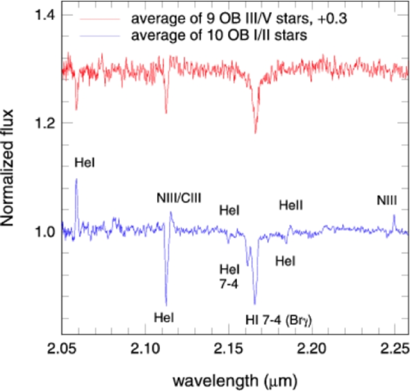
Figure 2: Left: Co-added, normalized and baseline subtracted spectra of the 10 best OB Iab–II supergiants (bottom) and the 9 best O III–V (top) stars in our sample. For each star we determined the velocity and then shifted all stars to a common rest frame. The various transitions are labeled. For the top spectrum a constant of 0.18 was added. Right: templates from Hanson et al. (2005) are overplotted on our spectra.

Figure 2 shows the co-added spectra of the 10 best OB I stars and the 9 best O III/V stars. A comparison with the atlas of Hanson et al. (2005) shows that these two sample average spectra are very similar to their respective solar neighborhood templates. After more than a decade of search, our data finally reveal the missing OB population in the Galactic Center. It is clear that the non-detection of these stars in earlier studies was merely an instrumental effect.

In addition to the 41 new OB stars outside the central 0.85″, we identify 30 post main-sequence blue supergiants and Wolf-Rayet stars, adding several stars to the sample already known from previous work (Genzel et al. 1996, 2000, 2003; Paumard et al. 2001). Of these, we classify 17 as Ofpe/WN9 and late nitrogen rich WRs (WNL=WN7–9) stars, and 12 as carbon rich WRs (WC) stars. There is one early WN (WNE, WN5/6) star, IRS 16SE2. The Northern Arm bow-shock star IRS 1W, with Br$\gamma$ in emission and He I $\lambda$ 2.058 µm in absorption as only features, is perhaps a Be star (see Paumard et al. 2004a for spectrum and detailed discussion). There is also one additional tentative WC candidate (IRS 7SE2).

Tanner et al. (2006) classify the 6 bright Ofpe/WN9 (narrow emission line stars and LBV candidates from Paumard et al. 2001) as B stars on the basis that they do not detect N III $\lambda$ 2.116 µm emission in these stars. They also do not detect the He I complex at 2.113 µm for the variable star and best LBV candidate IRS 34W (Trippe et al. 2005), in contrast to the other 5. However we clearly detect these features although the He I feature is mostly in emission (with some P Cyg absorption) in IRS 34W (see spectra in Paumard et al. 2004b and Trippe et al. 2005).

Hanson et al. (1996) have suggested that these very bright stars in the IRS 16 cluster might be OBN stars. OBN stars are particular kinds of O and B stars which show unusually strong N lines in the optical. They are also known to show unusually strong He lines, and to be particularly bright because of a lower atmospheric opacity (Langer 1992). Indeed, the strengths of the 2.115 µm N III compound and the 2.163 µm He I 7–4 absorption, relative to Br$\gamma$, in the average spectrum of the newly detected supergiants in Fig. 2 suggests that many of the luminous OB stars in the central parsec are nitrogen and helium rich. An extreme case is IRS 16CC where the He I absorption line at 2.163 µm is almost as deep as the Br$\gamma$ line. The only stars of the Hanson et al. (1996, 2005) atlases to show comparable depth in He I $\lambda$ 2.163 µm are HD 191781 and HD 123008, two ON9.7 Iab stars. Detailed modeling of our new stars is ongoing (Martins et al. 2006). Preliminary results seem to confirm a He enrichment (He/H$\simeq 0.3\pm 0.1$) for the ‘average’ star. This is still compatible with standard evolutionary models with rotation, though. Based on simple morphological arguments, the stronger absorption in He I $\lambda$ 2.163 µm in IRS 16CC and IRS 16SSE2 may indicate an even larger helium enrichment, which could be in conflict with theoretical predictions. More work is definitely needed to draw any reliable conclusion.

All these evolved stars are included in Tables 2 and 3. In total, Table 2 lists 90 certain detections of early type stars. Table 3 has an additional 14 further candidates. More than 100 early-type stars have now been detected in the nuclear star cluster, and this number is expected to grow in the next years.

3.2 Dynamics of the Young Stars

3.2.1 Two Disks of Early Type Stars

Genzel et al. (1996) were the first to note that the twenty or so bright ‘HeI’ emission line stars between $p=1\arcsec$ and 12″ known at that time exhibit a coherent rotation pattern in their radial velocities. Stars north of the center are blue-shifted while stars south of the center are red-shifted. This pattern is opposite to Galactic rotation. Genzel et al. (2000) and Paumard et al. (2001) confirmed and extended these findings. Adding proper motions to the radial velocities allowed a more constrained analysis (Genzel et al. 2000, 2003; Levin & Beloborodov 2003). In the end, Genzel et al. (2003) considered 26 stars with 3D velocity. They used $j$, the normalized angular momentum with respect to the line of sight, to demonstrate the existence of two coherent star systems (Appendix B, eq. B1) on near tangential orbits in projection ($|j|\simeq 1$), one rotating clockwise ($j\simeq+1$), the other counter-clockwise ($j\simeq-1$). Using a $\chi^{2}$ argument proposed by Levin & Beloborodov (2003; eq. B2), they show that both systems fit disk solutions. 12–14 stars form the clockwise system. It is rather thin and its midplane has an inclination of $i=120\arcdeg\pm 7\arcdeg$ with respect to the plane of the sky and a half-line of ascending (=receding) nodes at $\Omega=120\arcdeg\pm 15\arcdeg$ east of north (the actual numbers quoted in Genzel et al. 2003 are different because of different conventions; a detailed definition of those used in the present paper is given in Appendix A). The corresponding normal vector is $\mbox{\boldmath{$n$}}=(n_{x},n_{y},n_{z})=(-0.43,-0.75,+0.50)\pm(0.23,0.17,0.11)$. This system is the one found earlier by Levin & Beloborodov (2003). The second, counter-clockwise system in Genzel et al. (2003) is new, counts 10–12 stars, is thicker, and has $i=40\arcdeg\pm 15\arcdeg$ and $\Omega=160\arcdeg\pm 15\arcdeg$ ($\mbox{\boldmath{$n$}}=(-0.6,-0.22,-0.77)\pm(0.25,0.23,0.17)$). The two systems are at large angles relative to each other ($87\arcdeg\pm 36\arcdeg$). Tanner et al. (2006), adding 7 radial velocities and improving on others, also fit disk solutions on their data (10 stars in the clockwise system, 5 in the counter-clockwise). They find disk solutions in good agreement with their predecessors: $\mbox{\boldmath{$n$}}=(-0.42,-0.65,+0.76)\pm(0.05,0.03,0.06)$ and $(-0.23,-0.08,-0.97)$ $\pm 0.13$ (after normalization). From the rather high reduced $\chi^{2}$ they get, they conclude that the disks must be somewhat thicker than previously thought, although they make no quantitative statement.

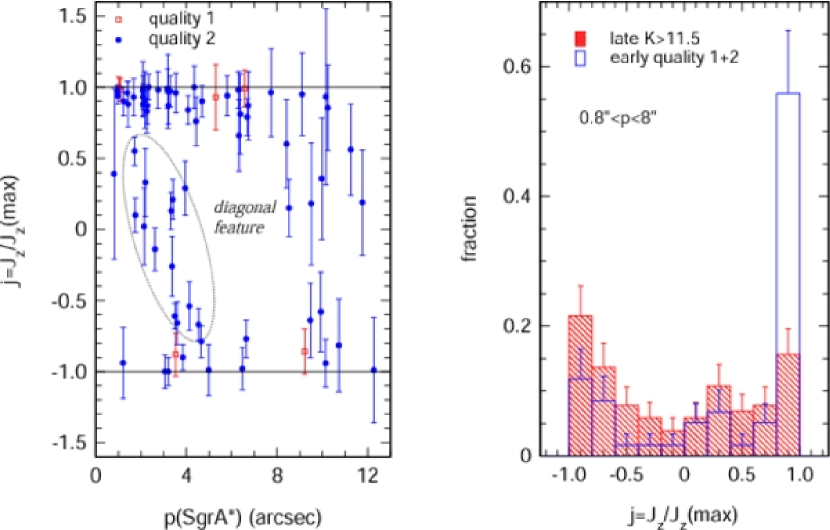
Figure 3: Left: Distribution of projected and normalized angular momentum on the sky $j=J_{z}/J_{z,\mathrm{max}}$ (eq. B1) for the early type stars as a function of projected separation $p$ from Sgr A* (for $p>0.8\arcsec$). In this diagram stars on projected tangential, clockwise orbits are at $j\simeq+1$ while stars on tangential, counter-clockwise orbits are at $j\simeq-1$. Stars at $j\simeq 0$ are on projected radial orbits. Filled circles denote the highest quality (2) spectroscopic stars and open squares denote moderate quality (1) stars. A diagonal feature (DF) is apparent on this diagram. It seems statistically significant, but we have no physical unique interpretation to suggest. Right: histogram of the $j$ distribution of the quality 1–2 spectroscopic stars integrated over $0.8\arcsec<p<8\arcsec$ ($N=59$), compared to a sample of $N=102$ $m_{K}>11.5$ spectroscopic late type stars that should be close(r) to relaxation.

Our new data increase the number of stars and the quality of the velocity measurements very substantially. In Fig. 3 we plot the same $j$ vs. $p$ (the projected distance from Sgr A*) diagram as in Genzel et al. (2003), adding our new stars. We exclude stars in the central ‘S’-cluster ($p\leq 0.8\arcsec$) that appear to be on randomly oriented, elliptical orbits (Ghez et al. 2005; Eisenhauer et al. 2005). For $p\geq 8\arcsec$ the velocities are smaller and proper motion uncertainties increase. As a result the typical uncertainty in $j$ increases to $\pm 0.3$–0.5 and a detailed analysis is not possible. For this reason we consider in the right panel of Fig. 3 the histogram of $j$ values for the 59 quality 1+2 stars for the range $0.8\arcsec\leq p\leq 8\arcsec$. We compare the distribution for the early type stars to the distribution of 102 late type stars with $m_{K}>11.5$ in the same range, which serve as a template for a relaxed distribution. 81% of the early type stars move on near-tangential orbits ($|j|>0.6$). This is to be compared to 59% for the late type stars. Early type stars clearly are preferentially on tangential orbits.

The clockwise system (CWS) at $j\simeq+1$ is particularly striking and now contains 36 (40) quality 1+2 stars with $|j|\geq 0.6$ and $p\leq 8\arcsec$ (14″). The counter-clockwise system (CCWS) is less well populated with 12 (17) stars with the same quality criteria and limits as above. In fact compared to the late type distribution in the right hand inset of Fig. 3 the enhancement in counter-clockwise stars at $|j|\geq 0.6$ would not appear statistically significant. We show below, however, that the counter-clockwise stars do indeed lie in a common plane, just as the clockwise stars and in contrast to the late type stars selected with the same criteria. There are $\simeq 10$ stars at $p<8\arcsec$ with small projected angular momentum. Of these, several have large error bars in $j$ and could still be part of the two tangential systems. However, it is interesting to note that these $\simeq$10 stars with $0.8\arcsec<p<8\arcsec$ and $|j|<0.6$ lie with a fairly small scatter around a diagonal line that runs from $(p=0\arcsec,j=0.6)$ to $(p=6\arcsec,j=0)$. Therefore this group of stars seems to have some statistical significance, although its physical meaning is not yet clear. We will later refer to these stars as the diagonal feature (DF) stars, as they share other noteworthy characteristics.

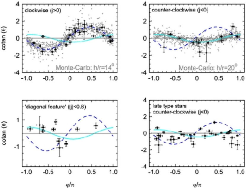
Figure 4: Location of various stellar populations in the $\varphi$–$\mathrm{cotan\,}\theta$ plane described in Sect. 3.2.1 and Appendix B (eq. B6): upper-left: clockwise early-type stars ($j>0$); upper-right: counter-clockwise early type stars ($j<-0$); lower-left: diagonal feature stars (see Fig. 3: $|j|<0.6$, $p<8\arcsec$); lower-right: counter-clockwise late type stars. Thick dots are quality 2 stars with $>3.5\sigma$ (average) detections of the 3 space velocities and (except for the DF stars) determination of $j$. Thin open circles are stars that have somewhat relaxed significance criteria ($2\sigma$). The thick dashed line is the best fitting clockwise disk ($i=124\arcdeg$, $\Omega=99\arcdeg$) and the thick continuous line is the best fitting counter-clockwise disk ($i=24\arcdeg$, $\Omega=167\arcdeg$). The small crosses denote Monte-Carlo simulations ($\simeq 10^{3}$ stars) of two disks with these parameters and a Gaussian distribution of opening angles ($\sigma=14\arcdeg$ and $20\arcdeg$ respectively).

The $\chi^{2}$ approach used by Levin & Beloborodov (2003) and Genzel et al. (2003) has the drawback that it is somewhat indirect. In the following we will use a different way of looking for disk structures in our stellar data. This new method is easy to visualize and can demonstrate the existence of a disk independently from the determination of its parameters. We show in Appendix B (eq. B6) that, in the plane spanned by $\varphi$ and $\mathrm{cotan\,}\theta$ ($\varphi$ and $\theta$ being the spherical coordinates of the velocity vectors), stars located in a planar structure must exhibit a telltale cosine pattern. Figure 4 shows the results if stars are coarsely separated into CWS, CCWS and DF stars. Beside the value of $j$ ($j<0$ for CCWS, $j>0$ for CWS, and $|j|<0.6$ for DF stars), the only criteria we used was the quality of the data for selection (or rejection), as determined from the average significance of the 3 space velocities $(\sum_{k=x,y,z}v_{k}/\sigma_{vk})/3$ and the significance in the determination of $\mathrm{sign\,}j$ ($j/\sigma_{j}$), and the projected distance $p$ from Sgr A*. As velocities decrease with $p$ and proper motion uncertainties increase with $p$, the quality of the velocity and $j$ determinations decrease with $p$. We find that quality 2 stars with velocity and $j$ significances $>3.5\sigma$ give by far the best determination of $\varphi$ and $\theta$. This essentially selects stars at $|j|>0.6$ and $p<7\arcsec$ into the two tangential systems. The DF is defined only by $|j|<0.6$ and $p<8\arcsec$. In addition we also considered more relaxed selection criteria ($\geq 2\sigma$). Our main finding is that there definitely are two well defined planar structures, at large angles with respect to each other ($115\arcdeg\pm 7\arcdeg$), in the early type star data. One at $i=127\arcdeg\pm 2\arcdeg$ ($1\sigma$), $\Omega=99\arcdeg\pm 2\arcdeg$ ($\mbox{\boldmath{$n$}}=(-0.12,-0.79,0.60)\pm 0.03$) fits all the clockwise stars with our quality criteria but one, which is indeed a DF star (3). Again, this is the clockwise disk already found by Levin & Beloborodov (2003).

The second structure at $i=24\arcdeg\pm 4\arcdeg$, $\Omega=167\arcdeg\pm 7\arcdeg$ ($\mbox{\boldmath{$n$}}=(-0.40,-0.09,-0.91)\pm(0.07,0.06,0.03)$) fits the all the counter-clockwise stars (a few appear as outlyers but they have large error bars). This second plane is coincident with the second plane identified by Genzel et al. (2003). Remarkably it also fits very well 8 of the 11 DF stars. 4 of the DF stars are compatible with both disks, 1 fits the CWS much better, and 1 (IRS 16SSW) appears to fit neither. Several of the 5 DF stars that fit best the CCWS have $j>0$, and therefore seem to counter-rotate in the disk in which they fit best, but $j<0$ is not excluded by more than $\simeq 1.5\sigma$.

Table 4: Planar Structures in the Galactic Center

Name	$\Omega$	$\pm$	$i$	$\pm$	$n_{x}$	$\pm$	$n_{y}$	$\pm$	$n_{z}$	$\pm$	Ref.
CWS	99	2	127	2	-0.12	0.03	-0.79	0.03	+0.60	0.03
CCWS	167	7	24	4	-0.40	0.07	-0.09	0.06	-0.91	0.03
Galaxy	31.4	0.1	90	0	+0.85	1e-3	-0.52	1e-3	+0.00	0.00	1
Northern Arm	15	15	50	30	+0.74	0.34	-0.20	0.28	-0.64	0.40	2
Bar	115	$\cdots$	76	$\cdots$	-0.41	$\cdots$	-0.88	$\cdots$	-0.24	$\cdots$	3
CND	25	$\cdots$	70	$\cdots$	+0.85	$\cdots$	-0.40	$\cdots$	-0.34	$\cdots$	4

Note. — The parameters listed here are defined in Appendix A. They give the orientation of the given disks as two angles, and as one normal vector. Values from other papers have been translated into our conventions.

References. — (1) Reid & Brunthaler (2004); (2) Paumard et al. (2004b); (3) Liszt (2003); (4) Jackson et al. (1993).

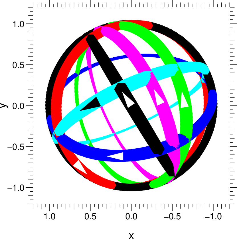
Figure 5: Various planar structures in the Galactic Center (Table 3.2.1): the Galaxy and sky (black), the clockwise (blue) and counter-clockwise (red) stellar systems, the Northern Arm (green) and Bar (cyan) components of the ionized mini-spiral, and the circum-nuclear disk (CND) of molecular gas (magenta). Each plane is represented by one ring. The thickness of the ring figures the proximity to the observer. Arrows indicate the direction of rotation.

Most of the bright stars in the so-called ‘IRS 16’ complex a few arcseconds east and south-east of Sgr A* are part of the clockwise system. This includes IRS 16C and IRS 16SW. Several stars in the IRS 13E complex, as well as IRS 16NE and IRS 16NW are part of the CCWS. In Table 3.2.1, we list the various planar structures in the Galactic Center, including the clockwise and counter-clockwise systems. Figure 5 illustrates the relative orientation of these planes. Although the CND and the Northern Arm of Sgr A West are at relatively low inclination to the plane of the Galaxy, it is clear that the two stellar disks, the Bar of Sgr A West and the Galactic plane are all quite different from each other.

Basically the same results are obtained from the alternative and independent method of Levin & Beloborodov (2003; eq. B2). For the CWS, this method gives $i=124\arcdeg\pm 2\arcdeg$ and $\Omega=100\arcdeg\pm 3\arcdeg$ and for the CCWS $i=30\arcdeg\pm 4\arcdeg$ and $\Omega=167\arcdeg\pm 9\arcdeg$.

Beloborodov et al. (2006, submitted) make a detailed analysis of the innermost region of the CWS ($p<5\arcsec$) using the “orbital roulette” method (Beloborodov & Levin 2004), which allows them to derive an independent estimate of the mass of Sgr A*. This part of the CWS appears quite thin: $10\pm 4\arcdeg$. The best fit plane is then $\mbox{\boldmath{$n$}}=(-0.14,-0.86,+0.50)$. In Table 2, we list the $z$ coordinate they derive for this solution.

3.2.2 The Disks Have Moderate Geometric Thickness

The best fit $\chi^{2}_{\mathrm{r}}$ values range between 2.3 and 3.1 for both disk systems, and for both equations B6 and B2. The disks are very well defined but the data require a finite thickness. If lower quality stars are added for the fitting the resulting $\chi^{2}_{\mathrm{r}}$ increases to values above 4. We interpret this effect as likely being caused by additional systematic uncertainties in velocity determinations, especially for stars at $p>6\arcsec$ and for stars with poorer or broader spectral features.

We have carried out Monte-Carlo simulations to determine the geometric thickness of the disks. We computed the location of $\simeq 10^{3}$ stars each in the ${\varphi}$–$\mathrm{cotan\,}\theta$ plane, assuming a normal distribution for the orbital inclinations to the system’s midplanes. We have varied the $\sigma_{i}$ width of these distributions and also taken into account the errors in the velocity determinations. We then compared the resulting model disks with the data to determine the best fit distributions (Fig. 4). For the clockwise set the best fitting value is $\sigma_{i}=14\arcdeg\pm 4\arcdeg$ ($\langle|h|/R\rangle=0.12\pm 0.03$). For the best 11 counter-clockwise stars, the best fit thickness is $19\arcdeg\pm 10\arcdeg$ ($\langle|h|/R\rangle=0.16\pm 0.06$). The two stellar disks have significant but moderate geometric thickness.

3.2.3 Steep Radial Density Profile and Inner Cutoff

We have estimated the 3D position of each star by assuming it is on the corresponding system’s midplane or, in other words, under a a very thin disk model assumption. The thickness of the disk introduces an error. The projected position on the CWS midplane of a CWS star at the average elevation is offset by $\simeq 0.1R$ perpendicular to the line of node ($0.07R$ for the CCWS). This effect can be in either direction though, depending on whether the star is in front or behind the midplane. Therefore, on average, this effect does not introduce a significant bias.

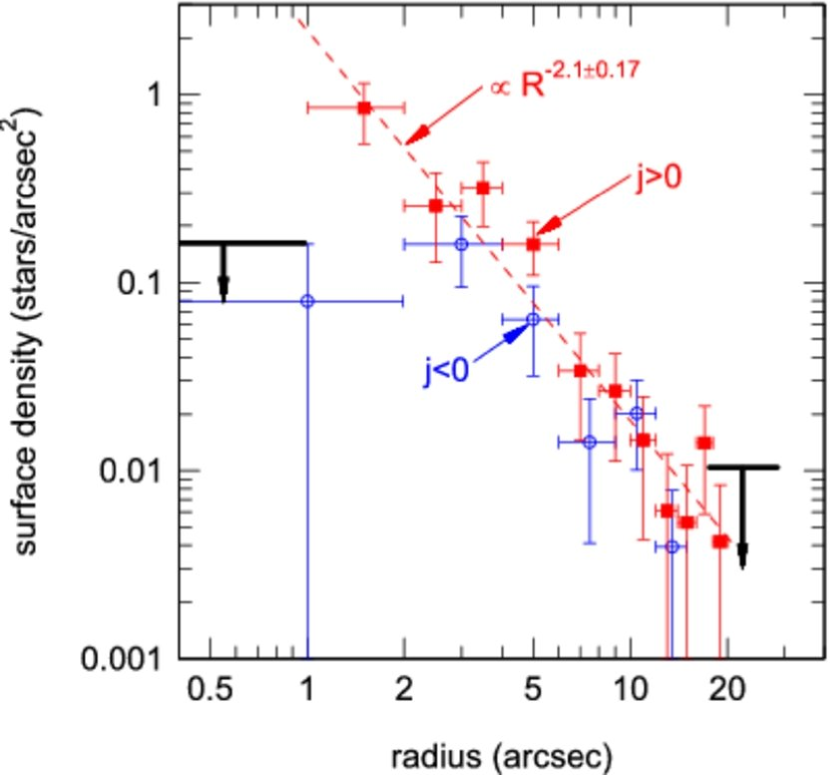
Figure 6: Surface density of stars in the clockwise (filled squares) and counter-clockwise (open circles) disk systems, as a function of 3D radius from Sgr A* and derived in the framework of a ‘thin disk’ model. The surface density distribution of the clockwise stars can be well fit by an extended disk with a sharp inner edge at $R\simeq 1\arcsec$ and a surface density decreasing outward proportional to $R^{-2}$. The counter-clockwise system more resembles a ring at $R\simeq 4\arcsec$ (or has a large inner edge of about $2\arcsec$) but with the same outward surface density falloff as the clockwise system. No OB stars are seen outside about $p\simeq 13\arcsec$ (Fig. 1) despite the deep continuous coverage in the northern strip and deep fields.

We have then calculated the surface density distribution as a function of true radius for stars with quality 2 and with $v$ and $j$ significance $>1.5\sigma$ in the clockwise and counter-clockwise systems. Figure 6 shows the results. The clockwise disk has a well defined power-law, surface density distribution with an index of $\simeq-2$. There is a very well delineated inner cutoff, at $p\simeq R\simeq 1\arcsec$. It is striking that this inner cutoff appears to coincide almost exactly with the outer radius of the central S-cluster of randomly oriented B-stars (Eisenhauer et al. 2005). The CCWS has a larger inner cutoff ($\geq 2\arcsec$) such that it appears to be more like a ring centered at $R\simeq 4\arcsec$, but this inner radius comes down to roughly the same as that of the CWS when including the DF stars ($0.8\arcsec<p<8\arcsec$ and $|j|<0.6$). Outside of this inner edge, however, its surface density distribution is very much the same as that of the clockwise system. The larger number of stars of the CWS as compared to the CCWS (excluding DF, factor $\simeq$2.5) thus is mostly the result of the former extending much further inward than the latter.

In addition to this, Fig. 1 shows already very clearly that the early type stars all reside in the central $p\simeq 13\arcsec$ ($\simeq 0.5$ pc) region despite our searches over a much larger region, and in several directions. This non-detection of OB stars is a quite robust result. In particular, in the strip stretching from $y\simeq 7\arcsec$ to $24\arcsec$ directly north of Sgr A*, the effective magnitude limit (for significant detection of spectroscopic features in early type stars) in this field is $\simeq$15.5 across the entire field ($\simeq$110 square arcseconds) and $>17$ in two deep subsections of about 20 square arcseconds (Maness et al. 2005, in preparation: Fig. 1). This region is close to the visible AO reference star so that the achieved Strehl ratio was high throughout the observations. Judging from the extinction map of Scoville et al. (2003) the excess K-extinction due to local dust is $<1$ mag throughout this region. This puts a 1${\sigma}$ upper limit of $\simeq 10^{-2}$ per arcsec² for O and early B stars outside the cutoff radius of $p\simeq 13\arcsec$. Over the $>200$ arcsec² region outside $p\simeq 13\arcsec$ covered by the shallower (spectroscopic K limiting magnitude $\simeq 13$) but wider large scale mosaics a similar limit is deduced. This upper-limit is consistent with, and strengthens, the $R^{-2}$ density profile extrapolated to $p>13\arcsec$.

3.2.4 Isotropic Azimuthal Structure

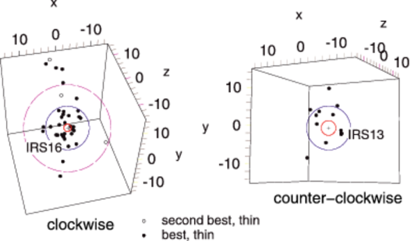
Figure 7: The azimuthal distribution of the stars in the clockwise ($j>0$, left inset) and the counter-clockwise ($j<0$, right inset) systems. Filled circles denote the positions of the best stars ($>1.5\sigma$ significance of z-determination) in the ‘thin disk’ model. Open circles denote the second best stars. The red circles denote the inner edges ($1\arcsec$ for the CWS, $2\arcsec$ for the CCWS). The blue and purple circles have radii of $6\arcsec$ and $12\arcsec$ respectively.

Figure 7 shows the azimuthal distribution of the stars in the clockwise and counter-clockwise systems when viewed from the pole of the two systems under the model assumption of very thin disks. Again, the radial distribution discussed in the last section, including the $\simeq 1\arcsec$ sharp inner edge of the CWS and the tendency of stars in the CCWS to be at large radii, perhaps in a ring-like shape, are apparent. The graphs also clearly show that the azimuthal stellar distribution is azimuthally symmetric to within the still fairly limited statistics of the data. Apparent local ‘concentrations’ exist but because of small numbers they are all consistent with statistical fluctuations.

This conclusion is somewhat in contrast to the work of Lu et al. (2005) who have argued that the concentration of 5 stars near IRS 16SW ($\simeq 1.5\arcsec$E, $1.5\arcsec$S of Sgr A*) may be the surviving core of a compact cluster. Their main argument is that the local 2D velocity dispersion is at a global minimum on this group. While a group of 4–6 stars corresponding to this ‘IRS 16 comoving group’ is clearly visible in the left inset of Fig. 7, to the left and down from center, there are similar such groupings elsewhere in the disk, of similar (low) statistical significance. However, what makes IRS 16 different from other locations in the field is the presence of a ‘hole’ in the CCWS at the same projected location (this hole also has very low statistical significance). Therefore, Lu et al. (2005) probably happen to be measuring the true velocity dispersion within the CWS at the location of IRS 16, whereas elsewhere, their measurement must include stars from the CCWS, and therefore naturally be higher.

Another interesting grouping of about 3 to 5 early type stars in a region of less than $1\arcsec$ is IRS 13E, $\simeq 4\arcsec$ south-west of Sgr A*, in the CCWS. This group has attracted recent interest, owing to the proposal by Maillard et al. (2004) that it may be stabilized against tidal disruption by an IMBH. We will return to this region in a separate section (3.3).

3.2.5 Circular and Non-Circular Motions in the Disks

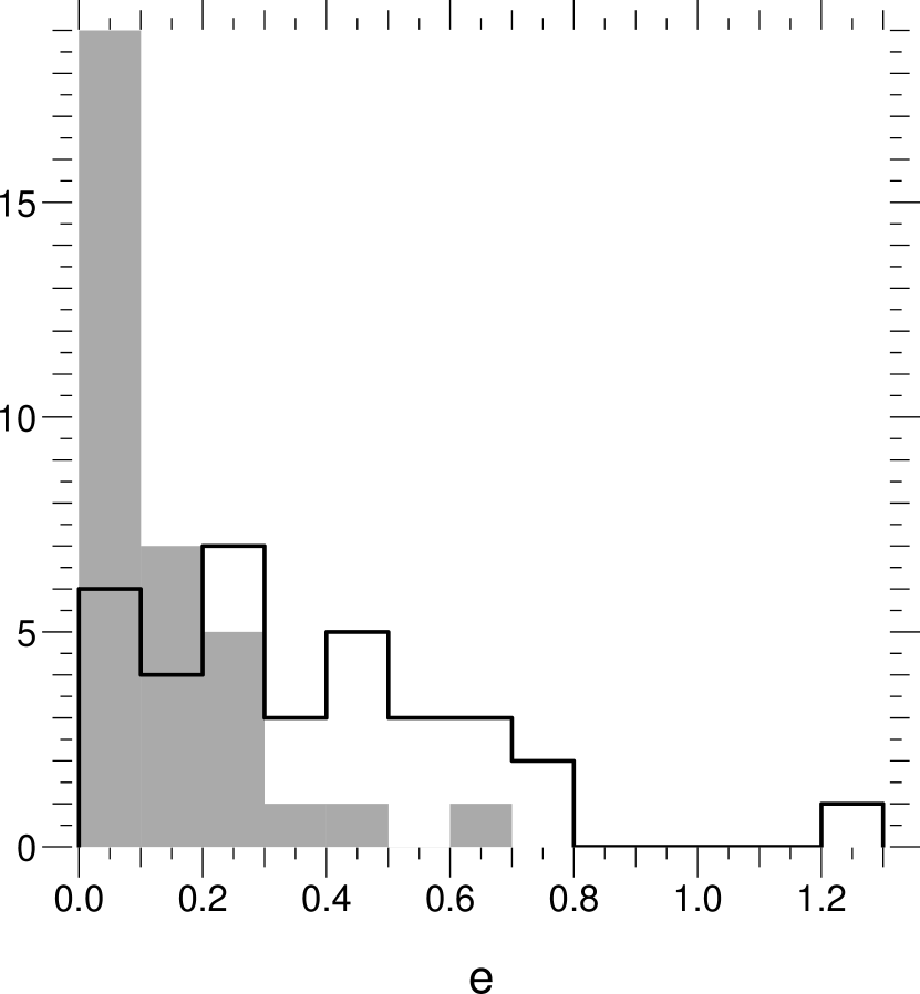
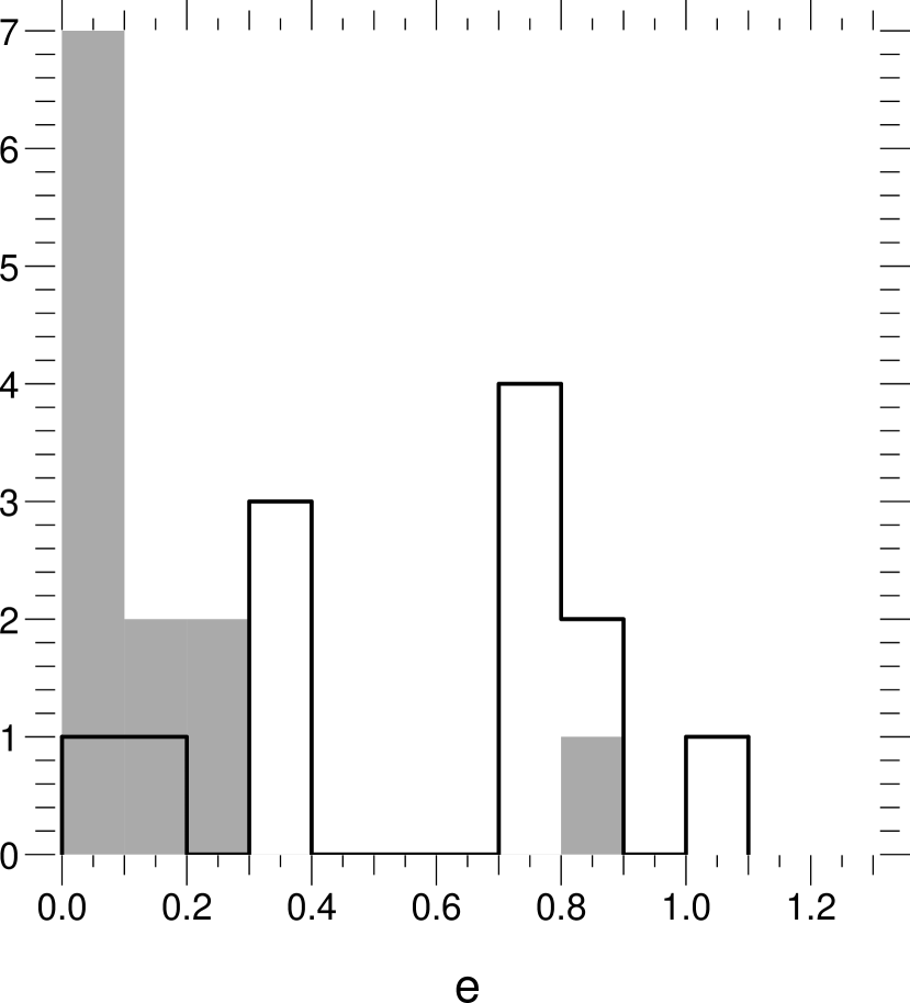
Figure 8: Eccentricity distributions in the CWS (left) and CCWS (right) disks, for both the real data sets (outlines; all stars with $v$ and $j$ significance $>2\sigma$) and artificial data sets for which all stars are assumed to be on circular orbits (filled histogram).

In this section we estimate the eccentricities of the stellar orbits in each disk. This eccentricity is straightforward to derive once the line-of-sight position ($z$) of a star is known (assuming the potential well and the distance to the GC, $R_{0}$, are known). We have used Monte-Carlo simulations to derive estimates of the eccentricity $e$ of each star, under the assumption that it belongs to one of the two disks. The method we used is described and discussed (including its limitations) in Appendix C. We produced artificial data sets under various assumptions to validate the method. The individual estimates we derive are listed in Table 2, and their histograms for the CWS and CCWS are shown on Fig. 8. The completely independent method used by Beloborodov et al. (2006, submitted) also allows them to derive stellar eccentricities. The two methods agree well on the individual values.

These histograms show that the distributions of eccentricities of the two systems are quite different. The CWS is made of stars on low to medium eccentricities ($\lesssim 0.5$). For this system, we find only slightly higher eccentricities than what we would derive for a system with the same geometry, on which all the stars would be on circular orbits. The distribution peaks around $e=0.2$, which is expected given the thickness of the disk ($\tan 14\arcdeg\simeq 0.25$). The CWS is essentially in low eccentricity, close to circular motion.

On the other hand, the CCWS contains a few low-eccentricity stars, including a peak around $e=\tan 19\arcdeg\simeq 0.35$, but is dominated by a high-eccentricity ($e\simeq 0.8$) population. Three of these stars belong to the IRS 13E complex (Sect. 3.3), but even when counting these three stars as a single dynamical entity, the conclusion remains that the CCWS is essentially in non-circular motion. The same work performed for the DF stars shows that if these stars live on either of the disks, then most of their eccentricities have to be quite high (very close to 1). These high eccentricity stars are definitely bound to Sgr A*.

3.3 IRS 13E: a dissolving star cluster and/or the site of an intermediate mass black hole?

The compact, bright source IRS 13E, $3\arcsec$ west and $1.5\arcsec$ south of Sgr A*, merits special discussion. IRS 13E has several properties that tend to make it unique in the central cluster. It

1. is associated with a bright peak of dust and ionized gas emission in the mini-spiral, at the edge of the so-called ‘mini-cavity’ (e.g. Clenet et al. 2004; Paumard et al. 2004b);

2. harbors at least $3$ bright stars within a radius of $0.25\arcsec$ (Paumard et al. 2001);

3. is associated with a point-like X-Ray source (Baganoff et al. 2003; Muno et al. 2005);

4. is associated with a compact centimeter radio source (Zhao & Goss 1998);

5. is dynamically coherent in that its bright early type stars participate in a similar 3D space motion (Maillard et al. 2004; Schödel et al. 2005).

Maillard et al. concluded that IRS 13E consists of at least 7 stars, out of which 4 have highly correlated sky velocities. From the radial velocity difference between two of the sources, they inferred an enclosed mass in excess of $10^{3}$ solar masses to bind the cluster. They argued that such a mass could not be accounted for by (lower mass) stars in the cluster and that the cluster might contain an intermediate mass black hole (IMBH) and be the remaining core of an in-spiraling star cluster disrupted in the central parsec and stabilized by this IMBH. On the basis of somewhat higher resolution images and more accurate proper motions Schödel et al. (2005), using 4 sources, concluded that IRS 13E could either be a local concentration of stars in the counter-clockwise disk or a dissolving cluster core. By setting a lower limit to the mass of a stabilizing intermediate mass black hole of $10^{4}M_{\sun}$ they felt that the presence of such an object is quite unlikely for two reasons. First, such a massive black hole is not easy to form as a result of core collapse even in a very massive ($10^{6}M_{\sun}$) in-spiraling cluster, as core collapse typically creates a central concentration no more massive than $\simeq 10^{-3}$ of the original cluster mass (Portegies Zwart & McMillan 2002). Second, an intermediate mass black hole with a mass in excess of $10^{4}M_{\sun}$ would be inconsistent with the 2 km s^-1 proper motion velocity limit perpendicular to the Galactic plane deduced by the VLBA observations of Reid & Brunthaler (2004).

3.3.1 IRS 13E is not a background fluctuation

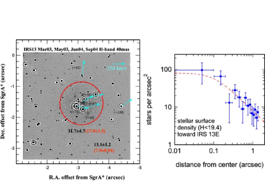
Figure 9: Left: Sensitive H-band image of the IRS 13E cluster region constructed from a combination of 4 NACO H-band data sets. The brightest stars have $m_{K}\simeq 10.7$ and the image has a dynamical range of $\simeq 9$ mags. The central circle centered on IRS 13E has a radius of $0.68\arcsec$. The main members of the IRS 13 group are labeled 1…6 (nomenclature of Maillard et al. 2004), with radial velocities given in parenthesis. Two other members of the counter-clockwise system are in the image and are also marked by their radial velocities. Arrows indicate direction and magnitude of proper motion (calibration in the upper right corner). The numbers next to the circle are the surface densities of stars detected within it with the STARFINDER (Diolaiti et al. 2000) algorithm to $m_{H}=20.4$ and (in parenthesis) $m_{H}=19.4$ ($m_{K}\simeq 18.5$ and 17.5), along with their 1${\sigma}$ uncertainties. For comparison, we list the surface densities (and uncertainties) to the same limits for the rest of the image shown. Right: surface density of stars to $m_{H}=19.4$, as a function of separation from the center of IRS 13E at $x=-3.12$, $y=-1.57$. The dotted curve is fit to a cluster with density profile $\propto 1/(r^{2}+r_{\mathrm{core}}^{2})$ and core radius $r_{\mathrm{core}}=0.17\arcsec$.

In the following we will first use a statistical approach to determine through stellar counts whether the IRS 13E group can be a chance association of stars in projection. Figure 9 shows a very deep H-band image we have constructed from a combination of four high quality NACO images in 2003 (March and May) and 2004 (June and September). Each of these images was individually ‘cleaned’ from the ‘dirty’ AO PSF with the Lucy-Richardson algorithm and then re-convolved with a 40 mas FWHM Gaussian. For this purpose we constructed a template PSF from isolated bright stars across the $\simeq 3.5\arcsec$ field. The co-added image was then again deconvolved with a Wiener filter with a PSF constructed from fainter isolated stars immediately around IRS 13E. The final image shown in Fig. 9 has a dynamical range of 9 mag and the faintest significant stars have equivalent K-magnitudes of $\simeq 19.5$. We then used STARFINDER (Diolaiti et al. 2000) to find and determine the photometry of all stars in the field. We computed the surface densities for a circular aperture of radius $0.68\arcsec$ centered on and encompassing the core of IRS 13E, as well as for the rest of the $3.2\arcsec\times 3.2\arcsec$ region shown in the figure. Fig. 9 lists the surface densities (and their ${1\sigma}$ uncertainties) to an H-magnitude limit of 20.4 ($m_{K}\simeq 18.5$). In parentheses we also give the same results for the more conservative limit of $m_{H}\simeq 19.4$. The stellar surface density in the central aperture ($31.7\pm 4.7$ ($17.9\pm 3.5$) stars per arcsec²) is 2.3 times greater than in the surrounding region ($13.1\pm 1.2$ ($7.9\pm 0.94$) stars per arcsec²).

Evaluating the significance of this result requires the careful use of Poisson statistics given our prior knowledge. This computation is done in Appendix D. We come to the conclusion that IRS 13E is very unlikely a background fluctuation (a quite conservative upper limit on the likelihood that this is the case is 0.2%). We thus concur with Maillard et al. (2004) that IRS 13E is very probably a local overdensity of stars in the CCWS. We further note that the surface densities given above for the center of IRS 13E are higher than anywhere but in the central cusp within $0.7\arcsec$ of Sgr A* (Fig. 7 in Schödel et al. 2006, in prep.). There, the surface density to $m_{H}=19.4$ is $32.3\pm 4.7$ stars per square arcsecond, 1.8 times the value toward IRS 13E. Because of the crowding it is not possible to estimate an $m_{H}<20.4$ surface density toward Sgr A*. Toward the center of the IRS 16 region, for instance, the surface densities to $m_{H}=20.4$ (19.4) are $11.4\pm 1.3$ ($9.3\pm 1.2$) stars per square arcsecond, rather similar to the average background density surrounding IRS 13E.

3.3.2 The IRS 13E cluster is on an eccentric orbit

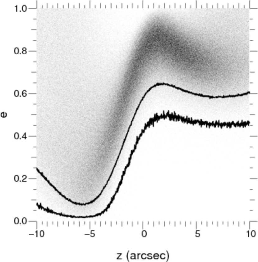
Figure 10: Monte-Carlo simulation of the eccentricity of the IRS 13E group motion. Given the known distribution of probability for the accessible parameters ($R_{0}$, $M_{\mathrm{SgrA*}}$, $x$, $y$, $v_{x}$, $v_{y}$, $v_{z}$), we have computed the distribution of probability for $e$ as a function of $z$ (shading). The two curves trace the 2 and $3\sigma$ lower limits on $e$. The map is not corrected for the low number depletion issue (Appendix C). The data would be compatible with circular motion if $z\simeq-5\arcsec$.

We now return to the remarkable deviation from circular motion of IRS 13E as estimated from the Monte-Carlo simulations in the last section (3.2.5). In the context of the cluster scenario it is now possible to average the space motions of the 4 bright stars of IRS 13E and obtain a more precise estimate for the motion of the cluster: $(x,y)=(-3.12\arcsec\pm 0.10\arcsec,-1.57\arcsec{\pm}0.12\arcsec)$, $(v_{x},v_{y},v_{z})=(-253\pm 62,57\pm 48,98\pm 21)$ km s^-1. We have also some more information on the line-of-sight position of the cluster. First, three of the four bright stars in IRS 13E (13E2, 3 and 4) are formally in the counter-clockwise system (CCWS). 13E1 is formally a DF star, and is also compatible with the CCWS (at high eccentricity, though). In the framework of this disk, IRS 13E is at $z\simeq 1.5\arcsec$. Second, Paumard et al. (2004) argue that IRS 13E is physically close to the ‘Bar’ component of the ionized mini-spiral, which they demonstrate is somewhat behind Sgr A*. Furthermore Liszt (2003) proposes a model of the Bar as a ring orbiting Sgr A* at 0.3–0.8 pc ($7.7\arcsec$–$20\arcsec$), which would put IRS 13E at $z=6.8\arcsec$–20″. It seems therefore rather safe to assume that IRS 13E is at positive $z$. A distance of $z\simeq 7\arcsec$ be in reasonable agreement with both constraints (proximity to the Bar and to the CCWS), with an orbial inclination to the CCWS midplane $i_{\mathrm{CCW}}\simeq 1.8$–4.2 ($1\sigma$) times the CCWS half opening angle. The same Monte-Carlo approach as in Sect. 3.2.5 allows us to estimate the eccentricity of the orbital motion of the cluster around Sgr A* as a function of $z$ (Fig. 10). Since we have just shown that IRS 13E lies on the right-hand side of this diagram, we can conclude that it is on a fairly eccentric orbit, with $e\gtrsim 0.5$.

3.3.3 Does IRS 13E Contain an IMBH?

We now ask the question of whether this cluster can be stable without an IMBH at its core. The two elements to check are the tidal forces from Sgr A* and the internal velocity dispersion. The distribution of stellar surface density as a function of distance from the center of IRS 13E reveals a very small effective core radius (at which the surface density has fallen to half its central value), $r_{\mathrm{core}}\simeq 0.17\arcsec$ (0.0066 pc or 1,400 AU, Fig. 9). After subtraction of the background, we count 12 stars to $m_{H}=19.4$ within $\simeq 0.35\arcsec$ ($\simeq$2 core radii). For the very simplified assumption that these stars sample the mass function to $\simeq 5.5M_{\sun}$ (ZAMS for $m_{H}\simeq 19.4$ at $A_{K}\simeq 3.2$) and adopting a flat mass function with $\mathrm{d}N\simeq m^{-1.35}\mathrm{d}m$ (Sect. 3.5), the inferred stellar mass within that radius is about $350\pm 100M_{\sun}$. For such a flat mass function the difference between that mass and the mass extrapolated to $1M_{\sun}$ amounts to about 30 solar masses only. On the other hand, stellar crowding is an issue. Our star counts are unlikely to be complete in the very center of IRS 13E and in the vicinity of its brightest stars. Thus our mass estimate is obviously a lower limit to the total stellar mass associated with the cluster, and the derived core radius is probably an upper limit. The core density of IRS 13E ($>3\times 10^{8}M_{\sun}$ pc^-3) is higher than in any other known cluster, except the cusp around Sgr A*.

IRS 13E is currently at $\gtrsim 4\arcsec$ from Sgr A*. At this distance, the tidal (‘Hill’) radius for such a mass is

$$r_{\mathrm{Hill,IRS13E}}=\left(\frac{M_{*}}{M_{\mathrm{BH}}}\right)^{1/3}R=0.13\arcsec M_{*400}^{1/3}$$ (1)

where $M_{*}$ is the mass of the star cluster, $M_{\mathrm{BH}}$ the mass of Sgr A*, and $M_{*400}=M_{*}/400M_{\sun}$. The Hill radius is in remarkably close agreement with the observed core radius. However, the distance to take into account is not the current one, but the periapsis distance. This parameter is poorly constrained from our Monte-Carlo simulations. It appears that if the cluster were would be on the CCWS midplane, then the periapsis would be fairly small and the required cluster mass high ($\gtrsim 10^{4}M_{\sun}$). On the other hand, requiring IRS 13E to be (currently) close the the Bar as discussed above allows the periapsis distance to be easily above $4\arcsec$. In this case, the inferred stellar concentration toward IRS 13E may thus be stable against tidal forces, or at least relatively long-lived, without the need for an IMBH.

It is interesting to note that, with the same constraints on the current line-of-sight position as above, we can estimate the date of the last periapsis passage of IRS 13E to be $\simeq 400$–$1000$ yr ago. It is therefore possible that the past event of AGN activity of Sgr A* 300–400 year ago (Revnivtsev et al. 2004) was linked with the passage of IRS 13E at its periapsis.

The main argument in Maillard et al. (2004) and Schödel et al. (2005) in favor of high cluster masses ($10^{3}$ and $10^{4}M_{\sun}$ respectively) came from the velocity dispersion inside the cluster. We still have 3D velocities only for four ‘stars’ in the cluster, one of which, IRS 13E3, is not even a single object but the red core of the cluster, resolved as two sources (3A and 3B) in Maillard et al., and that we see as no less than seven source in the present work. This source should therefore be discarded from velocity dispersion analyses, and we remain with only 3 stars. Our study shows that even though IRS 13E constitutes an over-density in the central parsec, more than one star out of three in the aperture do belong to the background population rather than to the compact cluster. For this reason, any measurement of the velocity dispersion should be considered with caution. In particular, IRS 13E1, which drives the high value found by Schödel et al. (2005), is formally a DF star rather than a CCWS star and has (when studied independently) a higher eccentricity than the other 13E stars. It is possible that this star is not bound to the cluster. We thus take the conservative position that the evidence for a central dark mass in IRS 13E from the proper motion data presently is not strong.

3.3.4 Formation Scenario

Although the IRS 13E over-density and the ring-like structure of the CCWS centered on the radius of IRS 13E may appear to favor a dissolving cluster scenario, it is also compatible with the idea of a star cluster formation in situ, within an accretion disk or dispersion ring. If IRS 13E has grown from gravitational instability in the original counter-clockwise gas disk the maximum ‘isolation mass’ that could have collapsed to the present cluster is approximately the mass contained within the annulus of radial thickness $2~{}r_{\mathrm{Hill}}$,

$$M_{\mathrm{isolation}}=A\,M_{\mathrm{disk}}^{3/2}M_{\mathrm{BH}}^{-1/2}\;,$$ (2)

where A is between 4 and $\simeq$30 (Lissauer 1987; Milosavljevic & Loeb 2004). Taking a disk mass of $5000M_{\sun}$ (Sect. 3.5) and $M_{\mathrm{BH}}=4\times 10^{6}M_{\sun}$ this isolation mass is at least $700M_{\sun}$. Our estimated stellar mass thus is also consistent with the concept of local cluster formation within the counter-clockwise disk, in agreement with the proposal by Milosavljevic & Loeb (2004).

Overall, it appears that the various pieces of evidence argue for a cluster mass of order $10^{3}M_{\sun}$, and that this mass can consist in stars, without a black hole. There is some indication, but no firm evidence, for a higher mass. In particular, if IRS 13E is a concentration in the CCWS, we would expect it to be close to the CCWS midplane. This would require a mass $\gtrsim 10^{4}M_{\sun}$. Further progress will require more proper motions and radial velocities for the individual faint stars in the cluster.

3.4 Stellar Content: the Disks Are Coeval And $\simeq$6 Myr Old

Wolf-Rayet (WR) stars of different sub-types appear at different ages. The number ratios of these sub-types in a coeval population of stars thus give information on the properties of the star forming event leading to the observed population, in particular its age (Mas-Hesse & Kunth 1991, Vacca & Conti 1992, Schaerer et al. 1997). The evolution of massive stars and the presence of a WR phase are controlled by stellar winds, which depend on metallicity. In principle the number ratios of WR to O stars can thus also trace the metal content. However, the strong effects of rotation on the evolution of massive stars modify the duration of the different phases of massive star evolution, especially for the WR phases (Meynet & Maeder 2003; Maeder & Meynet 2004). Rotation varies from star to star, and the predicted number ratios are affected by this natural spread.

Table 5: Numbers and Fractions of Early Type Sub-Classes in the Two Disks

	clockwise			counter-clockwise
Type	Number	fraction	uncertainty	number	fraction	uncertainty
OB I/II	18	0.36	0.08	3	0.15	0.09
OB III/V	13	0.26	0.07	6	0.30	0.12
Ofpe/WNL	12	0.24	0.07	5	0.25	0.11
WNE	1	0.02	0.02	0	0.00	0.00
WC	6	0.12	0.05	6	0.30	0.12
Sum	50			20

Table 6: Ratio of Different Sub-Types

Type 1/ Type 2	Clockwise	Counter-Clockwise	All
WR/O	0.61	1.22	0.75
WR/(WR+O)	0.38	0.55	0.43
WNL/(WR+O)	0.24	0.25	0.24
WNE/(WR+O)	0.02	0.00	0.01
WC/(WR+O)	0.12	0.30	0.17
WC/WN	0.46	1.2	0.67

Tables 5 and 6 list the numbers and relative fractions of the different sub-types of early type stars in the two stellar disks. Compared to observations in other star forming regions, the WR/O star fraction in the Galactic Center disks is remarkably high. This is partly a selection effect: our number counts are more complete for the supergiants and WN stars than for the dwarfs, WC and WO stars. To first order, the fraction of different types of post main-sequence supergiants and WR stars is strikingly similar in the two disks. The fraction of OB (I–V) stars appears to be somewhat higher in the clockwise system, which may also have a marginally greater fraction of OB supergiants. The striking resemblance in content of massive stars strongly suggests that the two stellar disks are basically coeval (Genzel et al. 2003).

3.4.1 Population Synthesis

From these ratios, we can attempt to estimate the age and star formation history of the two disks. In order to investigate the physical properties of the stellar population more quantitatively, we computed population synthesis models for a determination of the expected number ratios under various conditions (star formation history, metallicity, initial mass function). Technical details on the method, based on the synthesis code developed by Schaerer & Vacca (1998), are given in Appendix E.

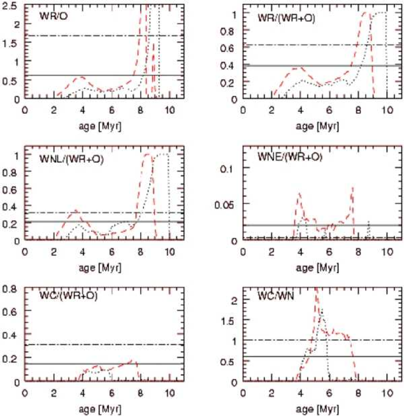
Figure 11: Number ratios of different types of massive stars as a function of time under the assumption of a single burst of star formation. The adopted initial mass function has a slope of 2.35, a lower mass limit of $1M_{\sun}$ and an upper mass limit of $100M_{\sun}$. We have used Geneva evolutionary tracks with rotation for solar (dotted line) and twice solar metallicity (dashed line). The horizontal solid lines correspond to the observed values and are upper limits. The second peak in the WR/O ratio is due to massive stars experiencing a blue loop.

The constant star formation case can easily be ruled out since none of the predicted number ratio matches the data. In particular, we do not detect any O3–6 stars. A burst of star formation is clearly preferred. Figure 11 shows the results for such a scenario and a Salpeter initial mass function (IMF). We see that the data are compatible with an age ranging between 4 and 9 Myr. In fact, most of the ratios point to an age of 7–8 Myr except WC/WN which is also compatible with younger ages ($\simeq$4–5 Myr). All ratios involving O stars are certainly upper limits, and as such indicate that the deduced age of 7–8 Myr is an upper limit.

The number ratios presented in Fig. 11 are usually higher when Z is larger. However, in most of these diagrams we see that the age derived from the solar metallicity case is similar to the one derived from the twice solar metallicity case. The only exception is the ratio WC/(WR+O) for which the $Z_{\sun}$ model predicts values lower than what we observe. This may be an indication that Z in the central cluster is slightly super solar, but given the uncertainty in the current observed number ratios of WR to O stars, this needs to be confirmed by much more robust analyses.

Choosing a burst of star formation with finite duration has the effect of shifting the time scale by 2 Myr but does not change significantly the shape of the function giving the number ratios as a function of time. We believe that a duration of ${\leq}$2 Myr is quite consistent with our data. Longer bursts would also create large numbers of red supergiants. Only three such supergiants (IRS7, IRS19 and IRS22, Blum, Sellgren & DePoy 1996) are observed in the central parsec.

As for the IMF, adopting a flatter one increases the strength of the first “bump” around 4 Myr observed in the evolution of the number ratios (Fig. 11), but does not strongly modify the ratios at later epochs. For a top-heavy IMF the number ratios of the CWS are consistent with a burst of star formation $\simeq$ 4 Myr ago (the solution at $\simeq 6$–7 Myr being still valid).

3.4.2 Hertzsprung-Russell diagram

We have also modeled the ages of the luminosity class I–V OB stars directly by placing them on an infrared (IR) Hertzsprung-Russell diagram and comparing the data with isochrones. This requires the knowledge of both an absolute luminosity (or magnitude) and effective temperatures for all stars (Appendix F). We restricted ourselves to the OB stars since for the evolved massive stars (Ofpe/WN9 and WR stars), no calibration of effective temperature as a function of spectral type exists (mainly due to the strong effect of winds on the stellar properties of such objects). We excluded from our analysis those stars for which the spectral classification is uncertain. We also excluded the S stars near the central black hole.

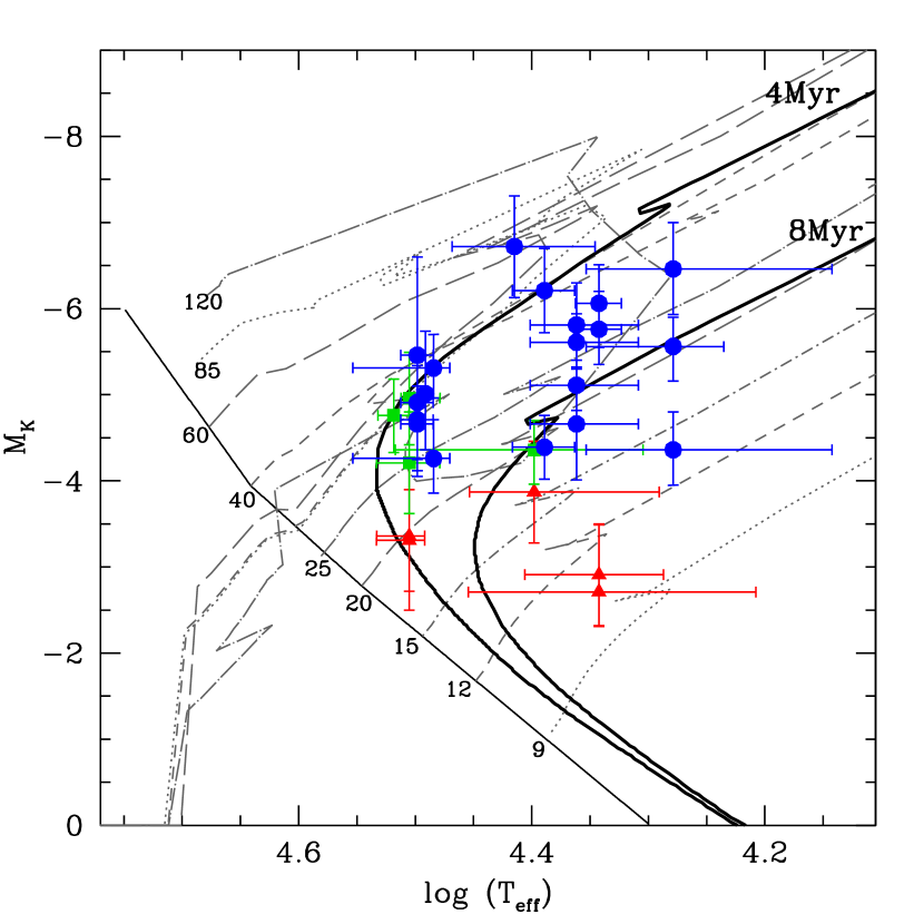
Figure 12: Location of the OB supergiants (blue dots), giants (green squares) and dwarfs (red triangles) in an IR Hertzprung-Russell diagram. The numbers indicate the initial mass of the star on the tracks starting from the ZAMS (thin solid line). The two thick solid lines are two isochrones for 4 and 8 Myr. The tracks (various dotted/dashed lines) are based on Geneva models without rotation (Lejeune & Shaerer 2001).

The results are shown in Fig. 12. Overplotted are Geneva evolutionary tracks taken from the database of Lejeune & Schaerer (2001). Isochrones for 4 and 8 Myr are also shown. We see that most of the stars are located between these two isochrones. In particular, there are no stars on the left side of the bend at $\log T_{\mathrm{eff}}\simeq 4.5$ in the 4 Myr isochrones, showing that the stellar population is older. There are a few outliers – though with large error bars – cooler than the 8 Myr isochrone, but an older age is not likely in view of the presence of numerous WR stars not included in this diagram for reasons highlighted above. The present age estimate confirms the result of the previous section. The OB population in the Galactic Center is 4 to 8 Myr old. The fairly large age uncertainties are inherent to our methods of assigning $M_{K}$ and $T_{\mathrm{eff}}$ (Appendix F). The fact that two different studies give the same result is rather convincing and reassuring.

In summary the stellar disks in the Galactic Center have formed about $6\pm 2$ Myr ago. They are coeval to within about 1 Myr. The burst duration did not exceed about 2 Myr. The present results thus are in excellent agreement with the earlier findings of Tamblyn & Rieke (1993) and Krabbe et al. (1995). Krabbe et al. invoked a decaying burst of star formation 7 Myr ago to explain the observed stellar population and its ionizing properties.

3.5 Flat Mass Function and Total Mass of the Stellar Disks

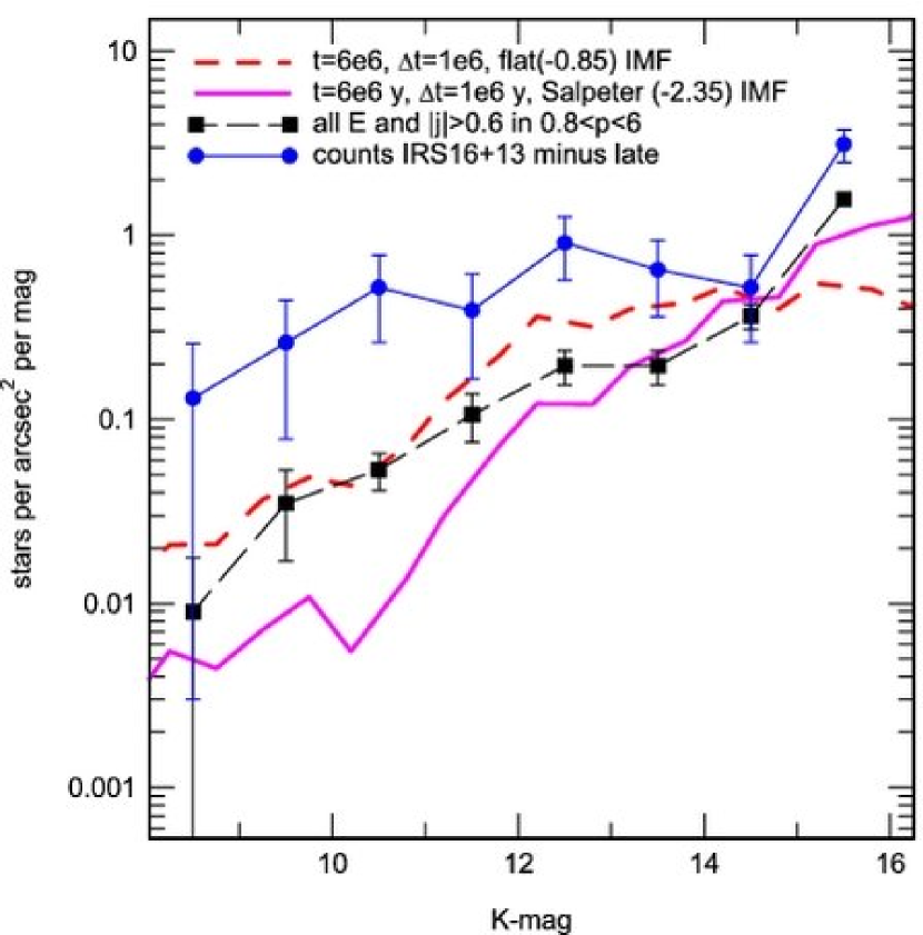
Figure 13: K-band luminosity function. Filled circles and squares denote two ways of estimating the K-band luminosity function of the early type stars. The filled circles denote counts from the best high resolution H/K-band NACO images in the IRS 16 and IRS 13 regions where spectroscopically identified late type stars have been eliminated. The filled squares denote all stars with $|j|>0.6$ and $0.8\arcsec<p<6\arcsec$ that are not spectroscopically identified as late type stars in our proper motion/spectroscopic catalogue (Ott et al. 2005, in preparation). The thick continuous curve represents the KLF of a $t=6$ Myr old cluster forming stars over ${\Delta}t=1$ Myr burst with Salpeter initial mass function ($\mathrm{d}N/\mathrm{d}m\simeq m^{-2.35}$), normalized to the average of the observed counts in the $m_{K}=14$–15 bin. The long-dashed thick curve denotes the KLF of a burst with the same age and duration as above, but with much flatter IMF ($\mathrm{d}N/\mathrm{d}m\simeq m^{-0.85}$).

In this section we use the stellar number counts as a function of K-magnitude to constrain the (initial) mass function of the young stars in the central parsec. In Fig. 13 we show two independent methods for estimating the K-band luminosity function (KLF) of the stars in the disks. Obviously the key issues are the screening against late type, background interloper stars and the determination of the number of early type stars at the fainter levels ($m_{K}>14$–15) where the spectroscopy is not yet possible or incomplete. Filled circles in Fig. 13 denote the KLF constructed from the deep counts from NACO H/K_s-band data in the IRS 16 region (size $2.5\arcsec\times 2.5\arcsec$) and IRS 13E cluster (size $0.7\arcsec$, see Fig. 9) and assuming that extinction is constant. We eliminated from those counts 11 stars which are spectroscopic late type stars but otherwise assume that the non-early type background toward these regions can be neglected. The steep rise in the counts probably indicates that this assumption is violated at $m_{K}>15$. Our alternative approach (filled squares) was to compute counts for the entire region $0.8\arcsec\leq p\leq 6\arcsec$ and require that the detected stars either are spectroscopic early type stars or (for the fainter stars) have $|j|>0.6$. This method thus suppresses the background by taking advantage of the tangential motion of most of the early type stars, in contrast to the late type stars (Fig. 3). Again, the steep rise of the counts at $m_{K}>15$ probably signifies a dramatic increase in the interloper background contribution. We note that for both methods the average ‘spectroscopic completeness limit’ is 13.5 to 14. The different slopes of the two observed luminosity functions in the spectroscopically ‘safe’ region at $m_{K}<13$ is possibly a result of a decrease in average stellar luminosity with $p$. The two methods more or less span the uncertainty box on the number of faint and bright stars to include in the luminosity function of the young stellar population. For comparison, the thick continuous and dashed curves show two model luminosity functions with different mass functions. Both curves are based on the population synthesis code STARS (Sternberg 1998; Sternberg, Hoffmann & Pauldrach 2003) with solar metallicity Geneva tracks and assume a burst model of age 6 Myr and duration 1 Myr compatible with the results of the last section. The continuous curve is for a standard 0.7–$120M_{\sun}$ Salpeter IMF ($\mathrm{d}N/\mathrm{d}m\simeq m^{-2.35}$), while the dashed curve is for a much flatter mass function ($\mathrm{d}N/\mathrm{d}m\simeq m^{-0.85}$). It is obvious that a Salpeter mass function cannot fit the very flat counts toward IRS 16/13E and does only marginally so for $m_{K}>12$. Both observed luminosity functions show a large excess above the Salpeter model for $m_{K}<11$. However, this range is dominated by very bright evolved stars that may not be properly accounted for by the Geneva tracks. Putting the largest weight on the more reliable range $11<m_{K}<14$, which includes the OB dwarfs and giants, we conclude that the data require a mass function flatter than a Salpeter function by $\simeq$1 to 1.5 dex.

With this result we can now estimate empirically the total stellar mass in the two stellar disks. As before, we exclude from the following discussion the cluster of B-stars in the central cusp around Sgr A*. There are in total $\simeq 53$ and 20 observed OB+WR stars (quality 1+2) in, respectively, the clockwise and counter-clockwise systems. Recent stellar evolution models with rotation by Meynet & Maeder (2003) and Maeder & Meynet (2004) indicate that only stars more massive than $\simeq 20$–$25M_{\sun}$ will go through the WR phase we observe in the Galactic Center. Likewise the faintest OB stars we are able to detect in the GC must have zero age main sequence masses in excess of about $20M_{\sun}$. We thus assume that the observed OB and WR stars represent the (initial) mass range of 20–$120M_{\sun}$. Adopting an initial mass function with a slope of $\Gamma=-1.35$ and -0.85 ($\mathrm{d}N/\mathrm{d}m=m^{\Gamma}$) required to fit the K-band luminosity function, the total mass in $\geq 20M_{\sun}$ stars is 2700–$3100M_{\sun}$ for the CWS and 1000–$1200M_{\sun}$ for the CCWS (the corresponding numbers for a Salpeter ($\Gamma=-2.35$) mass function would be 2100 and $790M_{\sun}$). Extrapolating from the number of $\geq 20M_{\sun}$ stars to the entire mass range above $\simeq 1M_{\sun}$ yields a total stellar mass of 3800–$3500M_{\sun}$ for the CWS and 1420–$1320M_{\sun}$ for the CCWS. Given that $\Gamma>-2$, these mass estimates are relatively insensitive to the choice of lower mass cutoff and slope. The corresponding numbers for a Salpeter mass function would be $10^{4}$ (CWS) and $3900M_{\sun}$ (CCWS). Obviously these estimates are lower limits since we almost certainly have not detected all the $M\geq 20M_{\sun}$ stars yet. We can establish a rough upper limit to the numbers of missing O stars by counting all stars ($0.8\arcsec<p<13\arcsec$) in our proper motion list (Ott et al. 2006, in preparation) that are on near tangential, clockwise orbits ($j>0.6$.) In Fig. 3 we showed that only $24\%$ of late type stars but $60\%$ of the early type stars reside in this range. Given that there are approximately the same number of late and early type stars ($\simeq 100$ each) to $m_{K}\simeq 13.9$, equivalent to an O8–9 V dwarf, the above criterion may select a sample with $\simeq 71\%$ early type stars. In our proper motion sample there are 35 such stars that are not spectroscopic early or late type stars. Hence an upper limit to the correction factor for missing early type stars with $M\geq 20M_{\sun}$ in each system is about $(53+0.71\times 35)/53=1.5$. We conclude that the total stellar content in the clockwise and counter-clockwise systems is $\leq 6000$ and $2200M_{\sun}$.

These estimates (or limits) are fully consistent with two other and completely independent lines of argumentation. In the first Nayakshin et al. (2005) consider the precession and warping that is induced by one of the stellar disks on the other, and vice versa. They study the evolution of the apparent thickness of the disks with time, as a function of their masses. They require the thickness to be as observed (Sect. 3.2.2) at $t=4$ Myr. Depending on whether the original configuration was two thin disks in circular motion, or whether the counter-clockwise disk was initially an in-spiraling cluster with significant radial motion, Nayakshin et al. find masses of between 5000 and $15,000M_{\sun}$ for the CWS and between 5000 and $10,000M_{\sun}$ for the CCWS. The 4 Myr age assumed in their work is somewhat smaller than what we deduced in Sect. 3.4. These masses thus are strict upper limits.

Nayakshin & Sunyaev (2005) havepointed out another argument for a flat initial mass function and for stellar masses $<10^{4}M_{\sun}$ owing to the weakness of extended X-ray emission in the central parsec. Nayakshin & Sunyaev argue that the bright X-ray emission of young T-Tauri stars is a handle for probing the low mass end of the mass function. For a $<10$ Myr old stellar component and a Salpeter mass function the predicted diffuse X-ray flux in the central parsec exceeds the observed value of Baganoff et al. (2003) and Muno et al. (2005) by a factor of 20 to 100.

From these various arguments it is safe to conclude that the mass function of the young stars in the Galactic Center is indeed flat and that the total stellar mass contained in the clockwise disk does not exceed $\simeq 10^{4}M_{\sun}$. The corresponding limit for the counter-clockwise system is probably $\simeq 5000M_{\sun}$. Our deep observations of the northern field (3.3.3 and Maness et al. 2005, in preparation) also strongly suggest that there is no ‘reservoir’ of B stars tidally stripped from the in-spiraling cluster at larger radii that would point to many missing lower mass stars. We thus believe that the flat mass function we, Nayakshin et al. (2005) and Nayakshin & Sunyaev (2005) deduce approximates an initial mass function, unaltered by dynamical effects.

4 Discussion

4.1 Origin of the Stellar Disks

What have we learned from the new observations and their analysis? Let us summarize the key conclusions:

1. the large majority of the early type stars in the central parsec (excepting those in the central cusp around Sgr A*) reside in one of two, well defined rotating disks. These disks are oriented at large angles with respect to each other, and to the Galactic plane. One rotates clockwise in projection, the other one counter-clockwise. The clockwise system (CWS) has 2.5 times as many massive stars as the counter-clockwise system (CCWS);

2. the disks have a well defined inner radius (edge). The more populated clockwise disk has an inner edge at $p=1\arcsec$, just outside the central B-star cluster in the Sgr A* cusp. Its azimuthal distribution is isotropic. The inner edge of the counter-clockwise disk is further out. This system thus resembles more a ring;

3. Both disks have an outer density profile scaling as $\Sigma\simeq R^{-2}$. No O/WR-stars (in all directions) and lower mass B-stars (toward the north) are present outside the central $p=13\arcsec$ region;

4. the disks have a finite but moderate thickness, $\sigma_{i}=14\arcdeg\pm 4\arcdeg$ ($\langle|h|/R\rangle 0.12\pm 0.03$) for the CWS and $19\arcdeg\pm 10\arcdeg$ ($\langle|h|/R\rangle=0.16\pm 0.06$) for the CCWS;;

5. almost all of the stars in the CWS are on low eccentricity, close to circular orbits;

6. on the contrary, most stars on the CCWS appear to be on eccentric orbits;

7. the IRS 13E group of early type stars appears to be the center of a larger local concentration of stars with ${\geq}$12 (K${\leq}$17.5) members and total stellar mass of order $10^{3}M_{\sun}$. It appears to have a large orbital eccentricity ($e>0.5$). This concentration represents the second largest stellar density in the central parsec, second only to the central Sgr A* cusp, and is among the highest known core densities ($>3\times 10^{8}M_{\sun}$ pc^-3). It is unlikely a projection effect. IRS 13E is compact enough that it may be long-lived in the tidal field of the central black hole, even without invoking a central intermediate mass black hole. It may be a slowly dissolving star cluster embedded in the counter-clockwise system;

8. the stellar disks are coeval to within 1 Myr, have an age of $6\pm 2$ Myr and must have formed over a time period $\leq 2$ Myr;

9. the total stellar mass associated with each of the two disks does not exceed $10^{4}M_{\sun}$;

10. the (initial) mass function of these disks is flatter than a Salpeter mass function by 1–1.5 dex.

Let us review the two star formation scenarios in view of this ‘report card’, for each of the two systems.

4.1.1 The In Situ Star Formation Scenario Is in Good Agreement with the Data

The presence of two well defined kinematical systems seems to require two separate events of star formation. This is actually somewhat problematic whatever the formation scenario is, since these two events must have occurred basically at the same time. However, the two events are allowed to be separated by $\simeq$1 Myr from each other. This timespan is sufficient for star formation to remove most of the gas from the first disk before the second one starts forming. The minimum time needed to form stars can be estimated as follows. Once the disk becomes gravitationally unstable, instabilities are believed to grow in the disk on dynamical time scale (e.g. Toomre 1964), i.e. $60\;\mathrm{yr}\;(R/1\arcsec)^{3/2}$. In addition to that, accretion of gas onto proto-stars is limited by the Eddington accretion rate onto these, which sets the stellar mass doubling time scale to about a thousand years (e.g., Nayakshin & Cuadra 2005). Taken together, these two conditions constrain the minimum duration of the star-formation episode to about $10^{4}$ yr. Therefore both gaseous disks are not required to have been in the central parsec at the same time. The in situ scenario passes points 1 and 8.

Points 2 and 3 are also reasonably natural in the context of an accretion disk. The minimum radius where the gravitational instability can form stars may be estimated as follows. In order for the disk to be self-gravitating at radius $R$, the accretion disk surface density $\Sigma_{\mathrm{gas}}$ must be larger than a minimum value (e.g. Fig. 2 in Collin & Hure 1999; Levin 2003, astro-ph/0307084), which is approximately given by $\Sigma_{\mathrm{min}}=10^{4}M_{4}M_{\sun}/(\pi R_{\mathrm{a}}^{2})$, where $M_{4}$ is the minimum unstable disk mass in units of $10^{4}M_{\sun}$ (see top panel in Fig. 1 in Nayakshin 2006, MNRAS, submitted, astro-ph/0512255), and $R_{\mathrm{a}}$ is the radius $R$ in arcseconds. At the same time, for a given dimensionless accretion rate $\dot{m}$, in units of the Eddington accretion rate, and the disk viscous $\alpha$-parameter, the standard accretion disk model (Shakura & Sunyaev 1973) predicts that $\Sigma_{\mathrm{gas}}=\Sigma_{\mathrm{SS}}\propto R_{\mathrm{a}}^{-3/5}$. Therefore, stars may be able to form only at disk radii greater than

$$R_{\mathrm{min}}\simeq 0.4\arcsec\alpha^{4/7}M_{4}^{5/7}\dot{m}^{-3/7}\;.$$ (3)

Given the crude nature of these estimates and uncertainties in $\alpha$ and $\dot{m}$, this estimate of $R_{\mathrm{min}}$ is reasonably close to the observed inner disk cutoff radius (precise values for both $\alpha$ and $\dot{m}$ are uncertain but should be reasonably close to unity in the case of a massive self-gravitating disk).

The radial stellar density profile $\Sigma$ may be expected to follow the initial gas surface density, $\Sigma_{\mathrm{gas}}$, if star formation instantaneously consumed most of the gas disk. Interestingly, the observed $\Sigma$ varies as $R^{-2}$, as expected in a

$$Q=\frac{c_{\mathrm{s}}\Omega}{\pi\mathcal{G}\Sigma}\simeq 1$$ (4)

marginally stable stationary self-gravitating disk (Lin & Pringle 1987; Collin & Hure 1999; Thompson, Quataert, & Murray 2005; $Q$ is the Toomre parameter, Toomre 1964). A time-dependent self-gravitating disk left to its own devices will also develop a steep surface density profile, $\Sigma_{\mathrm{gas}}\simeq R^{-3/2}$ (Lin & Pringle 1987), again close to the observed steep profile, especially when compared with the standard Shakura & Sunyaev profile that scales as $R^{-3/5}$ at large radii (when assuming a constant opacity, e.g. eq. 20 in Svensson & Zdziarski 1994). However, the time scales needed for the disk to go through a significant mass transfer in radial direction is prohibitively long:

$$t_{\mathrm{visc}} \simeq \Omega^{-1}\left(\frac{M_{\mathrm{BH}}}{M_{\mathrm{disk}}}\right)^{2}$$

$$\simeq 3\times 10^{8}\;\mathrm{yr}\;\left(\frac{R}{10\arcsec}\right)^{3/2}\left(\frac{M_{\mathrm{disk}}}{10^{4}M_{\sun}}\right)^{-2}\;,$$

where $\Omega$ is the Keplerian angular frequency.

The thickness (point 4) of the disks is also consistent with the expectations: even though the gas (and stellar) disks should be initially quite thin, they thicken somewhat due to relaxation ($h/R\simeq 0.1$ after a few $10^{6}$ yr, eq. 15 in Nayakshin & Cuadra 2005) and get warped due to the gravitational torque applied by each disk on the other one (Nayakshin & Cuadra 2005; Nayakshin et al. 2005). The low eccentricities of the orbits in the CWS (point 5) are the natural outcome from a marginally stable disk.

The disk mass necessary for a classical disk to fragment is $\gtrsim 10^{4}M_{\sun}$, just above the higher limit on the current stellar mass (point 9). This discrepancy is not worrisome. A fraction of the gas in the disks may have been expelled through stellar feed-back (either escaping the central region, or being redistributed and later accreted by Sgr A*). In addition, the disk surface density was perhaps not a smooth function of radius. In that case, the instability criterion $Q=1$ may have been reached in parts of a less massive disk, which would otherwise have been stable.

Formation of massive stars would not be unexpected in the accretion disk star formation scenario. The initial mass of the disk fragment collapsing to form first gravitational condensations in the disk should be of order $M_{\mathrm{frag}}=\rho_{\mathrm{disk}}h^{3}$, which can be estimated for the marginally self-gravitating disk at ($Q\simeq 1$) to be only $\simeq 0.01M_{\sun}$ (e.g., see the bottom left panel of Fig. 3 of Collin & Hure 1999. While their estimate was made for $M_{\mathrm{BH}}=10^{6}M_{\sun}$, $M_{\mathrm{frag}}$ is a weak function of the super-massive black hole mass). Nevertheless, since the requisite gas densities in the accretion disk are several orders of magnitude higher than even those in molecular cores, Bondi-Hoyle and Hill accretion rate estimates yield very high accretion rates onto these fragments, $\dot{M}>10^{-3}M_{\sun}$ yr^-1. With this stars double their mass at the rate limited by the Eddington limit, which is of order 1000 years (Goodman and Tan 2004, Nayakshin & Cuadra 2005, Fig. 2). Thus as little as $10^{5}$ years of such accretion would lead to very massive stars. In addition, stellar mergers could contribute to the growth of the massive stars. Finally, the first collapsed object may be more massive than the estimate above if radiative cooling rate is only marginally sufficiently fast to allow disk gravitational collapse (see, e.g. second simulation in Gammie 2001), or turbulent ‘pressure’ support is important in preventing smaller clouds to collapse (McKee and Tan 2004). For these reasons, a top-heavy mass fucntion (point 10) may be natural in the context of the in situ scenario. Future detailed work is warranted to delineate the dominant mode of massive star growth in the observed stellar disks.

Therefore, the in situ, accretion disk scenario fits perfectly for the clockwise system. There remains however two points to be clarified for the counter-clockwise system: the high eccentricity of the orbits (point 6), and the presence of a very dense star cluster (point7). At first glance these two points seem to be strong clues in the direction of the in-falling star cluster scenario. However, the latter point is resolved if the in situ model is amended with the possibility that gravitational collapse in the disk can lead to local cluster formation. The likely occurrence of this process has already been pointed out by Milosavljevic & Loeb (2004). The large eccentricities in the CCWS are not incompatible either with the accretion disk scenario. It is possible that that the progenitor accretion disk did not circularize before forming stars, since the disk fragmentation may have occured on a short dynamical timescale. Alternatively, gravitational interaction between IRS 13E and the gaseous disk may drive the former’s eccentricity (Goldreich & Sari 2003). Both of these ideas will be investigated in greater detail in the future. Overall, the in situ scenario seems acceptable for the CCWS, with some open theoretical questions.

4.1.2 The In-Spiraling Cluster Scenario Is Unlikely

The in-spiraling cluster scenario is also able to fulfill more or less easily most of the points of the ‘report-card’ above. The core density of IRS 13E ($>3\times 10^{8}M_{\sun}$ pc^-3) is greater than the core density required for a cluster to sink deep into the central parsec before disruption ($10^{7}M_{\sun}$ pc^-3). Nevertheless, the in-spiraling scenario seems to fail on point 3, and fails on point 9 in a way that we deem fatal.

First of all, models of such an in-falling cluster show that the cluster should lose a lot of stars during the inspiral, leaving a stellar population with a shallow radial profile extending over several parsecs in the radial direction, in contradiction to point 3. Gürkan & Rasio (2005) argue that this discrepancy can in principle be overcome by initial mass segregation in the cluster. In this way, the stars that are lost at large distance from the center are lower mass stars below our detection limit, and all the detectable stars are brought in the central parsec. No quantitative analysis has been done so far though, so that it is not clear whether the mass segregation–evaporation process can bring all the OB stars into the central 0.5 pc, with a density profile as sharp as the observed one, and not leave a telltale population of B stars at $R>0.5$ pc (which we do not observe).

Even if this strong mass segregation were possible, we would be observing all the $>20M_{\sun}$ stars initially in the cluster. The total inital mass of the cluster could not exceed $17\,000M_{\sun}$ for the CWS and $6,500M_{\sun}$ for the CCWS, even assuming a Salpeter IMF. The total mass required to make a cluster in-spiral from far out (a few $10$ pc) into the central region within an O star lifetime is $>10^{5}M_{\sun}$ (Gerhard 2001; McMillan & Portegies Zwart 2003; Kim et al. 2004; Gürkan & Rasio 2005). The inconsistency between the data and the models is a factor of $\gtrsim 6$ for the CWS, and $\gtrsim 15$ for the CCWS.

Therefore, taken together, these points favor strongly the in situ acretion disk model for the formation of both stellar disks in the central parsec. We conclude that the clockwise disk almost certainly resulted from in situ star formation in a dense gas disk. The most obvious process starting such a disk is the infall of a large gas cloud (Morris 1993; Genzel et al. 2003), followed by dissipation of its angular momentum through shocks in a ‘dispersion ring’ (Sanders 1998). The in situ star formation scenario is also plausible – and certainly much more plausible than the infalling cluster scenario – for the counter-clockwise system assuming that eccentric orbits and cluster formation can be understood within the framework of the model.

We do not have an explanation for the near-simultaneous occurrence of two star formation events 6 Myr ago, followed by little since then, and preceded by little for tens of Myr (Blum et al. 2003). It is unavoidable to conclude that the epoch 4–9 Myr ago must have been a very special one for the Galactic Center. It is interesting and relevant to note in this context that the other two young, massive star clusters in the central 50 pc, the Arches and Quintuplet cluster, have comparable stellar masses ($10^{4}M_{\sun}$), stellar content (WC/WN etc.), ages (2–7 Myr), and (flat) mass functions (Figer et al. 1999; Figer 2003; Stolte et al. 2005). We might speculate that star formation across the Galactic Center was triggered a few Myr ago by a global event, such as an interaction with a passing satellite galaxy that raised the pressure in the central interstellar medium and/or lead to increased cloud/cloud collisions.

4.2 Origin of the central B-star cluster by scattering from a sea of B-stars

We end by briefly commenting on the proposal of Alexander & Livio (2004) that the B-stars in the central cusp are the result of the capture of B-stars on near-loss cone orbits, originally unbound to the central black-hole, following a three body, direct exchange scattering process with the central massive black hole and $\simeq 10M_{\sun}$ stellar black holes residing in the central cusp.

This elegant and attractive proposal requires the presence of a ‘reservoir’ of B-stars originally at large distances from the central hole. In the specific model presented by Alexander & Livio (2004) the captured fraction of $\geq 3M_{\sun}$ B-stars is about $10^{-4}$ for a constant star formation scenario. With ${\geq}$15 B-stars presently observed in the central cusp (Eisenhauer et al. 2005), a total reservoir of about $1.5\times 10^{5}$ $\geq 3M_{\sun}$ B-stars (and $1.5\times 10^{4}$ ${\geq}15M_{\sun}$ stars) are required for the mechanism to work. The surface density in the reservoir depends on its spatial extent. Alexander & Livio (2004) consider stars originating between 0.5 pc (where stars are on unbound orbits relative to the MBH) to 2.5 pc (where the orbits are still marginally Keplerian), and find that the required surface density over that area is about 10 B stars per square arcsec. The deep observations reported toward the northern field (3.3.3) limit the number of $m_{K}<16.5$ B-stars to about 0.4 stars per arcsec². The discrepancy is a factor of 25. The current observations appear to to exclude the capture of unbound stars by the mechanism proposed by Alexander & Livio (2004). Alternatively the reservoir may be the stellar disks themselves. The exchange capture efficiency of such bound, short period stars is still under investigation. Due to crowding, it is not yet possible to securely identify B V stars, such as populate the S-cluster in the inner arcsec (Eisenhauer et al. 2005), throughout the disks. While it is possible that some of the stars we identify as OB III/V are B V stars (Table 5), deeper spectroscopy is required for a full census of the B V content of the disks.

5 Conclusions

We report firm spectroscopic detections of 41 OB stars (luminosity classes I–V) in the central parsec. The new data resolve a decade old puzzle of the ‘missing O stars’. Some of these stars seem He- and N-rich (OBN stars).

We confirm the presence and define the properties of the two young star disks first presented by Levin & Beloborodov (2003) and Genzel et al. (2003).

The disks rotate about the center and are at large angles with respect to each other. They have a very well defined inner radius, a radial surface density profile scaling as $R^{-2}$, and a moderate geometric thickness. In one of the disks (the clockwise, ‘IRS 16’ system) almost all stars are on close to circular orbits. However in the other, counter-clockwise, ‘IRS 13E’ system, most of the stars (including the IRS 13E cluster) orbit on eccentric orbits. Star counts suggest that IRS 13E is a long-lived cluster of stellar mass $\gtrsim 400M_{\sun}$. It is the cluster with the highest known core density after the cusp around Sgr A* itself: $>3\times 10^{8}M_{\sun}$ pc^-3.

The star disks are coeval within $\simeq$1 Myr and have formed $\simeq$6 Myr ago. The stellar mass function is significantly flatter than Salpeter, setting a limit to the total stellar mass in the disks of about $1.5\times 10^{4}M_{\sun}$.

The constraints just discussed strongly suggest that the stars in the ‘IRS 16’-disk were formed in situ from a dense gaseous accretion disk. They were not transported into the central parsec by an in-spiraling massive star cluster. On balance the same conclusion seems plausible (but not incontrovertibly proven) for the ‘IRS 13E’-disk. In that case, the IRS 13E cluster must have formed within the disk.

Appendix A Conventions used in this paper

We use the usual astronomical cartesian coordinate system, in offsets from from Sgr A*: $x=\cos\delta\mathrm{d}\alpha$ increases eastwards, $y=\mathrm{d}\delta$ increases northwards, and $z=\mathrm{d}D$ increases forward along the line-of-sight from the observer. We occasionally use spherical coordinates:

$$\varphi=\arctan\frac{y}{x}\;; \theta=\arccos(z/\sqrt{x^{2}+y^{2}})\;; R=\sqrt{x^{2}+y^{2}+z^{2}}\;$$ (A1)

$$x=R\sin\theta\cos\varphi\;; y=R\sin\theta\sin\varphi\;; z=R\cos\theta\;.$$ (A2)

When discussing orbital planes, we use the orbital elements defined in Aller et al. (1982), adapted for defining an oriented disk, which is consistent with Eisenhauer et al. (2005). The disks are first defined by the orientation of their line of nodes, which is the intersection of the disks (which contain Sgr A*) with the plane of the sky (also containing Sgr A*). More precisely, we refer to the ascending (=receding) half of this line. The position angle of the line of nodes ${\Omega}$ is the angle between the North direction and this ascending half of the line of nodes, increasing East of North (counter-clockwise). The second element necessary to define these oriented disks is the inclination $i$, measured on the ascending half of the line of nodes, from the direction of increasing ${\Omega}$ to the direction of motion on the disk.

$$0\arcdeg\leq i<90\arcdeg \Rightarrow \mathrm{counter-clockwise\;projected\;rotation;}$$

$$90\arcdeg<i\leq 180\arcdeg \Rightarrow \mathrm{clockwise\;projected\;rotation.}$$

An equivalent way to define these disks is to give the three Cartesian coordinates of their normal vector. The rotation of the stars on the disks is then always counter-clockwise when visualized from a point towards which the normal vector is pointing. A disk is counter-clockwise (in projection) when the $z$ coordinate of its normal vector is negative and clockwise when it is positive.

$$n_{x}=\sin i\cos\Omega\;;\;n_{y}=-\sin i\sin\Omega\;;\;n_{z}=-\cos i\;.$$ (A3)

The spherical coordinates of the normal vector relate to $i$ and $\Omega$, but are not equal to them:

$$\varphi_{\mbox{\boldmath{$n$}}}=-\Omega\;;\theta_{\mbox{\boldmath{$n$}}}=180\arcdeg-i\;.$$ (A4)

Appendix B Discriminating star disks

Genzel et al. (2003) defined the sky-projected angular momentum (or normalized angular momentum with respect to the line of sight) as

$$j=\frac{J_{z}}{J_{z,\mathrm{max}}}=\frac{xv_{y}-yv_{x}}{(x^{2}+y^{2})^{1/2}(v_{x}^{2}+v_{y}^{2})^{1/2}}\;.$$ (B1)

It is a simple way to distinguish stars on projected tangential orbits ($|j|\simeq 1$) from stars on projected radial orbits ($j\simeq 0$), and stars on projected clockwise orbits ($j\simeq+1$) from stars on projected counter-clockwise orbits ($j\simeq-1$). They fit disk solutions to the data by minimizing as a function of the normal vector $n$ the following quantity, introduced by Levin & Beloborodov (2003):

$$\chi^{2}=\frac{1}{N-1}\sum_{k=1}^{N}\frac{(\mbox{\boldmath{$n$}}\bullet\mbox{\boldmath{$v$}}_{k})^{2}}{(\mbox{\boldmath{$n$}}\bullet\mbox{\boldmath{$\sigma$}}_{k})^{2}}\;,$$ (B2)

where $\mbox{\boldmath{$v$}}_{k}=(v_{x,k},v_{y,k},v_{z,k})$ is the velocity vector and $\mbox{\boldmath{$\sigma$}}_{k}=(\sigma_{x,k},\sigma_{y,k},\sigma_{z,k})$ the corresponding velocity uncertainty of the $i$-th star ($Ox$ points Eastwards, $Oy$, Northwards, and $Oz$, away from observer). The unit vector $n$ describes the orientation of the normal vector to a common plane in which all $N$ stars are assumed to move.

There is a more straightforward way to find a disk in the data, which does not rely on fitting. Consider the 3D space velocity of star $k$ ($k=1{\dots}N$) in spherical coordinates (eqs. A1, A2),

$$\mbox{\boldmath{$v$}}_{k}=(v_{x,k},v_{y,k},v_{z,k})=||\mbox{\boldmath{$v$}}_{k}||(\sin\theta_{k}\cos\varphi_{k},\sin\theta_{k}\sin\varphi_{k},\cos\theta_{k})\;.$$ (B3)

Assuming that all $N$ stars are in the plane of a common disk with normal vector

$$\mbox{\boldmath{$n$}}=(n_{x},n_{y},n_{z})=(\sin i\cos\Omega,-\sin i\sin\Omega,-\cos i)$$

(see eq. A3), then all stellar velocity vectors must obey

$$0=\mbox{\boldmath{$n$}}\bullet\mbox{\boldmath{$v$}}_{k}=\sin i\cos\Omega\sin\theta_{k}\cos\varphi_{k}-\sin i\sin\Omega\sin\theta_{k}\sin\varphi_{k}-\cos i\cos\theta_{k}\;$$ (B4)

$$\sin i\sin\theta_{k}\cos(\Omega+\varphi_{k})=\cos i\cos\theta_{k}\;$$ (B5)

$$\mathrm{cotan\,}\theta_{k}=\tan i\cos(\Omega+\varphi_{k})\;.$$ (B6)

In the plane spanned by $\varphi$ and $\mathrm{cotan\,}\theta$, stars located in a planar structure thus must exhibit a telltale cosine pattern.

Appendix C The projection effects on the determination of the eccentricity

For the Monte-Carlo simulations in Sect. 3.2.5, for each star we assumed normal distributions for $v_{x}$, $v_{y}$, $v_{z}$, $R_{0}$ ($7.62\pm 0.32$ kpc, Eisenhauer et al. 2005) and $M_{\mathrm{SgrA*}}$ ($3.61\pm 0.32\times 10^{6}M_{\sun}$, Eisenhauer et al. 2005) ($x$ and $y$ have been left out as they play a minor role in the error budget). The potential well is assumed to be dominated by Sgr A*, which should essentially be true for the region where our measurements are most reliable ($p<8\arcsec$). We have drawn $z$ as a uniform variable ($|z|<20\arcsec$). For each one of the $10^{6}$ realizations (per star), we have computed the eccentricity $e$ and the inclination to the midplane of the system to which the star belongs ($i_{\mathrm{CW}}$ and $i_{\mathrm{CCW}}$, $i_{\mathrm{(C)CW}}$ for short). We then constructed the 2D histograms of these two parameters (maps of $P(i_{\mathrm{(C)CW}},e)$). In order to validate our method, we have performed the same analysis on several sets of artificial data that assumed a single eccentricity (including circular case) for all stars and the same geometry as the CWS and CCWS, introducing errors typical of the real systems. $R_{0}$ and $M_{\mathrm{SgrA*}}$ have been varied to check their influence on the conclusions.

In these 2D histograms, strong depletions where observed close to $e=0$ and $i_{\mathrm{(C)CW}}=0$. This is simply because of the uncertainties and of the functional dependency of $e$ and $i_{\mathrm{(C)CW}}$ on the 3D velocity (the true errors on $v_{x}$, $v_{y}$, and $v_{z}$ are unlikely to be all smaller than their respective $1\sigma$ error bar at the same time). We have approximately corrected this effect by dividing the histograms by ($1-\exp(-e/0.35)$) and ($1-\exp(-i_{\mathrm{(C)CW}}/20\arcdeg)$). This makes the 2D histograms look smooth and the values of $e$ determined for the artificial stars have the right statistics (peaking close to the assumed eccentricity). The correction affects only small eccentricities in practice ($e\lesssim 0.2$).

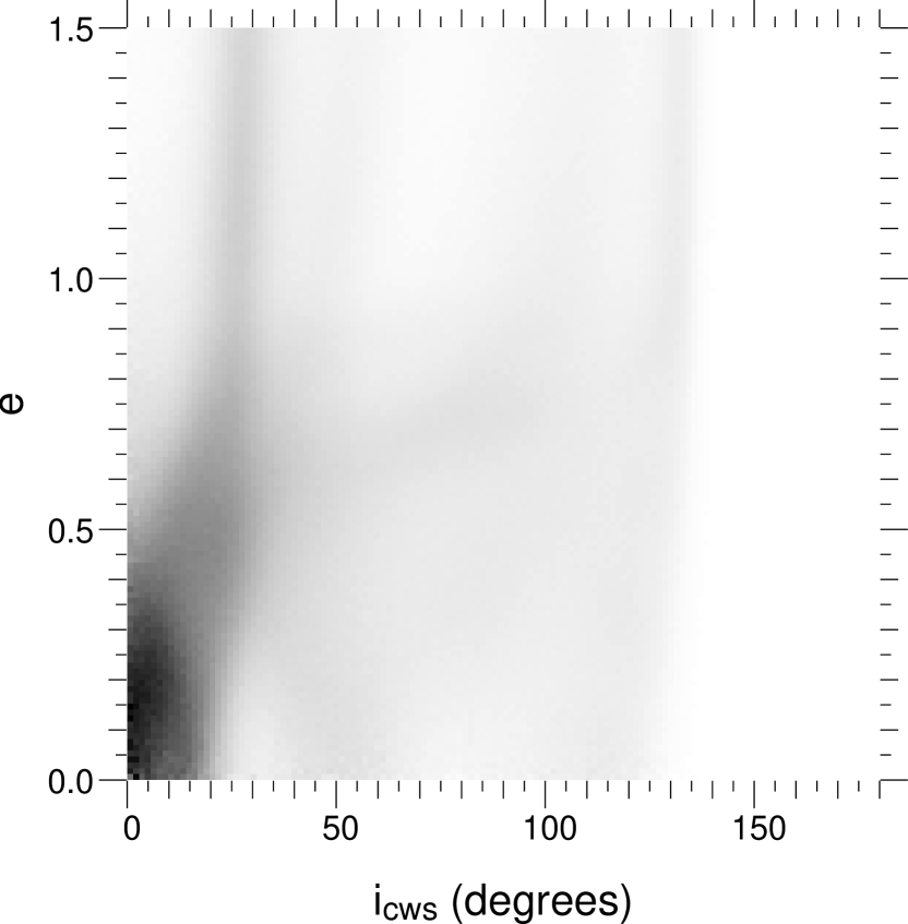
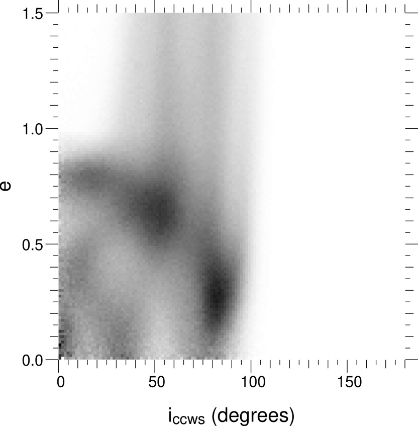
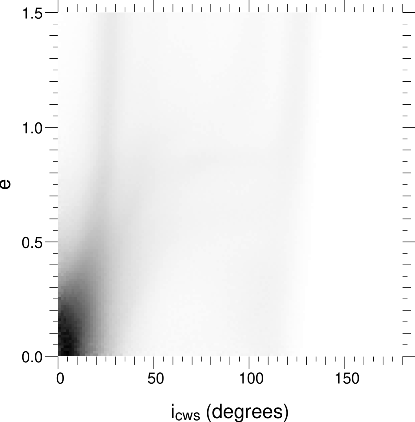
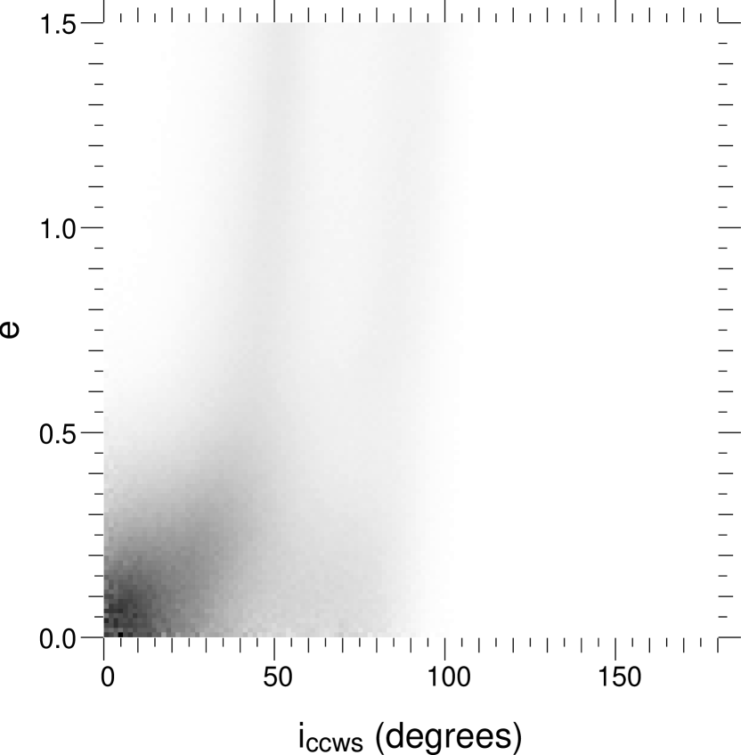
Figure 14: Co-added $e$ vs. $i_{\mathrm{(C)CWS}}$ 2D histograms $P(i_{\mathrm{(C)CW}},e)$ ($z$ uniformly distributed with $|z|<20\arcsec$, linear gray scale) for all stars in the following systems: real CWS and CCWS stars (top left and right; $p<8\arcsec$), artificial CWS and CCWS stars on circular orbits (bottom left and right). The real and artificial CWS maps are quite similar whereas the CCWS ones are very different from each other.

Figure 14 shows the sums of the histograms of all stars for each one of the CWS and CCWS, for both the real data and artificial data in which all stars are on circular motion. These co-added $e$ vs. $i_{\mathrm{(C)CW}}$ histograms yield a striking result: whereas the map for the CWS much resembles the corresponding artificial data set that assumes circular motion, with a maximum towards $(e=0,i_{\mathrm{CWS}}=0\arcdeg)$, this is not the case for the CCWS: for this system, the most prominent feature of the map is a (quarter of) ring running from $(e=0.8,i_{\mathrm{CCW}}=0\arcdeg)$ to $(e=0,i_{\mathrm{CCW}}=80\arcdeg)$. Such a ring-like structure on the 2D histogram of a star is the sign that this star can either be on the disk ($i_{\mathrm{(C)CW}}=0$) or on a circular orbit ($e=0$), but not both at the same time. Since indeed most of the maps of CCWS stars exhibit this ring, and since they can not be all at high inclination, we can already conclude that CCWS have typically high eccentricities.

From these maps, we can go further and estimate the eccentricity for each star. To do so, we simply compute (for each star) the distribution

$$P(e)=\int_{\mathrm{i(C)CW}}P(i_{\mathrm{(C)CW}},e)P(i_{\mathrm{(C)CW}})\mathrm{d}i_{\mathrm{(C)CW}}$$ (C1)

where $P(i_{\mathrm{(C)CW}})$ which is known a priori: a Gaussian centered on 0 and of width 14° and 19° respectively for the CWS and CCWS. We then fit a Gaussian on this distribution, and take the centroid as the best estimate, and the width of the Gaussian as the uncertainty.

It must be understood that the histograms are sometimes not nearly Gaussian. The method gives reasonable estimates given the quoted error bars, though.

Appendix D Likelihood that IRS 13E is a background fluctuation

In Sect. 3.3.1 we use stellar counts to show that IRS 13E is not a background density fluctuation. The first step is to determine the background density. We have made the approximation that, given ${\Lambda}$ the number of stars observed in the outside field of surface $A_{\mathrm{out}}$, the probability $P_{N}$ that the actual background density of stars is indeed $N$ per such area is given by a Poisson law of parameter ${\Lambda}$. In our case, $\Lambda=115$ to a limiting magnitude of $m_{H}=20.4$ ($69$ to $m_{H}=19.4$) and $A_{\mathrm{out}}=8.79$ arcsec².

Given $N$, the probability $P_{N\mathrm{in}|N}$ to find $N_{\mathrm{in}}=46$ (26) stars in the circular aperture of surface $A_{\mathrm{in}}=1.45$ arcsec² is also given by a Poisson law, of parameter $N\,A_{\mathrm{in}}/A_{\mathrm{out}}$. The probability, given our observations, that IRS 13E is but a spike in the Poisson noise of the background density of stars (i.e. a chance alignment) is given by the sum

$$\int_{N=0}^{+\infty}P_{N}P_{N\mathrm{in}|N}\mathrm{d}N\simeq\sum_{N=0}^{+\infty}P_{N}P_{N\mathrm{in}|N}\;.$$ (D1)

We find that the probability to find just by chance such a concentration of star at any randomly selected line-of-sight in the central parsec is $2\times 10^{-6}$ ($2\times 10^{-4}$). The over-density in IRS 13E is significant at the $4.5\sigma$ ($3.5\sigma$) level. Of course, if one selects a large number of lines-of-sight, the probability that one of these lines will be associated with such a chance over-density is higher than these numbers. The question thus arises whether the choice of the location of IRS 13E can be considered as random with respect to the problem of chance alignment of stars. As discussed in Sect. 3.3, the properties of IRS 13E make this source unique in the central parsec. However, one of the criteria for the selection of this field was the presence of three stars. Therefore, inasmuch as we subtract these three stars from our count numbers, we can consider the aperture around IRS 13E as randomly chosen. Given the number of stars that remain after having subtracted these three, the probability that the observed over-density associated with IRS 13E is but a chance alignment remains $2\times 10^{-5}$ ($2\times 10^{-3}$).

Appendix E Stellar Population Synthesis

We used the synthesis code developed by Schaerer & Vacca (1998). They distinguished several subtypes of Wolf-Rayet (WR) stars from O (and Of) stars. They defined any star burning H in its core and having effective temperatures larger than 33,000 K as an O star. Here we are more generally interested in a population of hot stars (O I–V + B I). We therefore modify their definition of an ‘O’ star to include the B supergiants, but not the B dwarfs, which we have not detected. In addition to this, the effective temperature of O stars has recently been revised downward (Martins et al. 2002, 2005; Crowther et al. 2002; Markova et al. 2004; Massey et al. 2005). In order to satisfy both points, we have considered as an ‘O star’ in the code every star with $T_{\mathrm{eff}}>23,000$ K and $\log L/L_{\sun}>5.2$. We used Geneva evolutionary tracks with rotation (Meynet & Maeder 2003; Maeder & Meynet 2004) for both solar and twice solar metallicity. We chose the minimum masses for WR stars according to the predictions of Meynet & Maeder (2003). An initial mass function with a minimum mass of $0.8M_{\sun}$ and a maximum mass of $100M_{\sun}$ was used, and we varied the slope between $-2.35$ (Salpeter) and $-1.35$ (top-heavy). We computed models for an instantaneous burst of star formation, an extended burst (2 Myr) and a constant formation rate.

Appendix F Determination of $T_{\mathrm{eff}}$ and $M_{K}$

Accurate $T_{\mathrm{eff}}$s are usually derived through detailed modeling of the spectra with atmosphere codes. This is a very long process, but first insights can be obtained with ‘effective temperature scales’ (c.f. Martins et al. 2005). In this way we were able to assign a spectral type to most of the stars observed so far. Absolute K band magnitudes can be easily computed from the observed K magnitudes, the distance to the Galactic Center and an estimate of the extinction. We used the currently best Galactic Center distance ($7.62\pm 0.32$ kpc, Eisenhauer et al. 2005). We applied the extinction map of Scoville et al. (2003) to estimate the K-band extinction $A_{K}$. To convert the V-band extinction $A_{V}$ into $A_{K}$, we have used the approximate relation $A_{K}\simeq 0.1A_{V}$. The resulting absolute magnitudes (and their ${1\sigma}$ uncertainties) are given in the last two columns of Table 2. For the 8 kpc distance adopted for the rest of this paper magnitudes would be increased by $\simeq 0.1$ mag. We applied the effective temperature scale of Martins et al. (2005) for O stars. For B stars we relied on the relations of Schmidt-Kaler (1982). In practice, for a star classified as 09–B1 I, we have chosen the effective temperature of a B0 supergiant as representative and the most likely range of values was chosen by adopting $T_{\mathrm{eff}}$s for a O9 and a B1 supergiant as limiting values.

References

- (1) Alexander, T. & Livio, M. 2004, ApJ, 606, L21
- (2) Alexander, T. 2003, in ‘The Galactic black hole’, eds. H.Falcke & F.W.Hehl, (Bristol: Inst. of Physics), 246
- (3) Alexander, T. 2005, Phys. Reports, 419, 65
- (4) Allen, D.A., Hyland, A.R. & Hillier, D.J. 1990, MNRAS, 244, 706
- (5) Aller, L.H. et al. 1982, in Landolt-Börnstein numerical data and relationships in science and technology, New Series, volume 2, subvolume b, Astronomy and astrophysics: Stars and star clusters, (Berlin: Springer), 382
- (6) Baganoff, F.K. et al. 2003, ApJ, 591, 891
- (7) Becklin, E.E., & Neugebauer, G. 1975, ApJ, 200, L71
- (8) Beloborodov, A. M., & Levin, Y. 2004, ApJ, 613, 224
- (9) Blum, R.D., Sellgren, K., & DePoy, D.L. 1995, ApJ, 440, L17
- (10) Blum, R.D., Sellgren, K., & DePoy, D.L. 1996, AJ, 112, 1988
- (11) Blum R.D., Ramirez, S.V., Sellgren, K., & Olsen, K. 2003, ApJ, 597, 323
- (12) Bonnet, H. et al. 2003, Proc. SPIE, 4839, 329
- (13) Bonnet, H. et al. 2004, The ESO Messenger, 117, 17
- (14) Collin, S., & Hure, J.-M. 1999, A&A, 341, 385
- (15) Clenet, Y. et al. 2004, A&A, 417, L15
- (16) Crowther, P.A., Hillier, D.J., & Smith, L.J. 1995, A&A, 293, 403
- (17) Crowther, P.A., Hillier, D.J., Evans, C.J., Fullerton, A.W., DeMarco, O., & Willis, A.J. 2002, ApJ, 579, 774
- (18) Davidson, J.A., Werner, M.W., Wu, X., Lester, D.F., Harvey, P.M., Joy, M., & Morris, M. 1992, ApJ, 387, 189
- (19) Davies, M.B., & King, A. 2005, ApJ, 624, L25
- (20) DePoy, D.L., Pepper, J., Pogge, R.W., Stutz, A., Personneault, M., & Sellgren, K. 2004, ApJ, 617, 1127
- (21) Dessart, L., Crowther, P. A., Hillier, D. J., Willis, A. J., Morris, P. W., & van der Hucht, K. A., 2000. MNRAS, 315, 407
- (22) Diolaiti, E., Bendinelli, O., Bonaccini, D., Close, L., Currie, D., & Parmeggiani, G. 2000, A&A Suppl., 147, 335
- (23) Eisenhauer, F., Schödel, R., Genzel, R., Ott, T., Tecza, M., Abuter, R., Eckart, A., & Alexander, T. 2003a, ApJ, 597, L121
- (24) Eisenhauer, F. et al. 2003b, The ESO Messenger, 113, 17
- (25) Eisenhauer, F. et al. 2003c, Proc. SPIE, 4814, 1548
- (26) Eisenhauer, F. et al. 2005, ApJ, 628, 246
- (27) Ekers, R.D., van Gorkum, J.H., Schwarz, U.J., & Goss, W.M. 1983, A&A, 122, 143
- (28) Figer, D.F., McLean, I.S., & Najarro, F. 1997, ApJ, 486, 420
- (29) Figer, D. F., Kim, S.S., Morris, M., Serabyn, E, Rich, R.M., & McLean, I.S. 1999, ApJ, 525, 750
- (30) Figer, D. 2003, Astr. Nachr. Suppl., 324, 255
- (31) Forrest, W.J., Shure, M.A., Pipher, J.L., & Woodward, C.A. 1987, in AIP Conference 155, The Galactic Center, ed. D. Backer (New York), 153
- (32) Genzel, R., & Townes, C.H. 1987, ARAA, 25, 377
- (33) Genzel, R., Thatte, N., Krabbe, A., Kroker, H., & Tacconi-Garman, L.E. 1996, ApJ, 472, 153
- (34) Genzel, R., Pichon, C., Eckart, A., Gerhard, O., & Ott, T., 2000, MNRAS, 317, 348
- (35) Genzel, R. et al. 2003, ApJ, 594, 812
- (36) Gerhard, O. 2001, ApJ, 546, L39
- (37) Gezari, S., Ghez, A.M., Becklin, E.E., Larkin, J., McLean, I.S., & Morris, M. 2002, ApJ, 576, 790
- (38) Ghez, A.M. et al. 2003, ApJ, 586, L127
- (39) Ghez, A.M. et al. 2004, ApJ, 601, L159
- (40) Ghez, A.M., Salim, S., Hornstein, S.D., Tanner, A., Morris, M., Becklin, E.E., & Duchene, G. 2005, ApJ, 620, 744
- (41) Goldreich, P., & Sari, R., 2003, ApJ, 585, 1024
- (42) Goodman, J. 2003, MNRAS, 339, 937
- (43) Goodman, J., & Tan, J. C. 2004, ApJ, 608, 108
- (44) Gould, A., & Quillen, A.C. 2003, ApJ, 592, 935
- (45) Gürkan, M.A., & Rasio, F.A., 2005, ApJ, 628, 236
- (46) Gürkan, M.A., Freitag, M., & Rasio, F.A., 2004, ApJ, 604, 632
- (47) Hall, D.N.B., Kleinmann, S.G., & Scoville, N.Z. 1982, ApJ, 260, L53
- (48) Hansen, B. M. S., & Milosavljevic, M., 2003, ApJ, 593, L77
- (49) Hanson, M.M., Conti, P.S., & Rieke, M.J. 1996, ApJ Suppl., 107, 281
- (50) Hanson, M.M., Kudritzki, R.P., Kenworthy, M.A., Puls, J., & Tokunaga, A.T.2005, ApJ Suppl., 161, 154
- (51) Herrero, A., Kudritzki, R.P., Vilchez, J.M., Kunze, D., Butler, K., & Haser, S. 1992, A&A, 261, 209
- (52) Horrobin, M. et al. 2004, Astr. Nachr., 325, 88
- (53) Jackson, J. M., Geis, N., Genzel, R., Harris, A. I., Madden, S., Poglitsch, A., Stacey, G. J., & Townes, C. H. 1993, ApJ, 402, 173
- (54) Kim, S. S., & Morris, M, 2003, ApJ, 597, 312
- (55) Kim, S. S., Figer, D. F., & Morris, M. 2004, ApJ, 617, L123
- (56) Krabbe, A., Genzel, R., Drapatz, S., & Rotaciuc, V. 1991, ApJ, 382, L19
- (57) Krabbe, A. et al. 1995, ApJ, 447, L95
- (58) Lacy, J.H., Townes, C.H., Geballe, T.R., & Hollenbach, D.J. 1980, ApJ, 241, 132
- (59) Langer, N. 1992, A&A, 265, L17
- (60) Lejeune, T., & Schaerer, D. 2001, A&A, 366, 538
- (61) Levin, Y., & Beloborodov, A.M. 2003, ApJ, 590, L33
- (62) Levin, Y., Wu, A.S.P., & Thommes, E.W. 2005, ApJ, 635, 341
- (63) Lin, D. N. C., & Pringle, J. E., 1987, MNRAS, 225, 607
- (64) Lissauer, J.J. 1987, Icarus, 69, 249
- (65) Liszt, H.S. 2003, A&A, 408, 1009
- (66) Lu, J.R., Ghez, A.M., Hornstein, S.D., Morris, M., & Becklin, E.E. 2005, ApJ, 624, L51
- (67) Maeder, A., & Meynet, G. 2004, A&A, 422, 225
- (68) Maillard, J.-P., Paumard, T., Stolovy, S. R., & Rigault, F. 2004, A&A, 423, 155
- (69) Markova, N., Puls, J., Repolust, T., & Markov, H. 2004, A&A, 413, 693
- (70) Martins, F., Schaerer, D. & Hillier, D.J. 2002, A&A, 382, 999
- (71) Martins, F., Schaerer, D. & Hillier, D.J. 2005, A&A, 436, 1049
- (72) Mas-Hesse, J.M., & Kunth, D. 1991, A&A Suppl., 88, 399
- (73) Massey, P., Puls, J., Pauldrach, A.W.A., Bresolin, F., Kudritzki, R.P., & Simon, T. 2005, ApJ, 627, 477
- (74) McMillan, S. L. W., & Portegies Zwart, S. F., 2003, ApJ, 596, 314
- (75) Meynet, G., & Maeder, A. 2003, A&A, 404, 975
- (76) Mezger, P.G., Duschl, W., & Zylka, R. 1996, A&A Rev., 7, 289
- (77) Milosavljevic, M., & Loeb, A. 2004, ApJ, 604, L45
- (78) Mokiem, M.R., de Koter, A., Puls, J., Herrero, A., Najarro, F., & Villamariz, M.R. 2005, A&A, 441, 711
- (79) Morisset, C., Schaerer, D, Bouret, J.C., & Martins, F. 2004, A&A, 415, 577
- (80) Morris, M. 1993, ApJ, 408, 496
- (81) Morris, M. & Serabyn, E. 1996, ARAA, 34, 645
- (82) Morris, P.W., Eenens, R.P.J., Hanson, M.M., Conti, P.S., & Blum, R.D. 1996, ApJ, 470, 597
- (83) Muno, M.P., Pfahl, E., Baganoff, F.K., Brandt, W.N., Ghez, A., Lu, J., & Morris, M.R. 2005, ApJ, 622, L113
- (84) Najarro, F., Hillier, D.J., Kudritzki, R.P., Krabbe, A., Genzel, R., Lutz, D., Drapatz, S., & Geballe, T.R. 1994, A&A, 285, 573
- (85) Najarro, F., Krabbe, A., Genzel, R., Lutz, D., Kudritzki, R.P., & Hillier, D.J. 1997, A&A, 325, 700
- (86) Nayaksin, S., & Cuadra, J.J. 2005, A&A, 437, 437
- (87) Nayakshin, S., & Sunyaev, R. 2005, MNRAS, 364, L23
- (88) Nayakshin, S., Dehnen, W., Cuadra, J., & Genzel, R., MNRAS, submitted
- (89) Ouellette, J. A., & Pritchet, C. J. 1998, AJ, 115, 2539
- (90) Ott, T., Eckart, A., & Genzel, R. 1999, ApJ, 523, 248
- (91) Paumard, T., Maillard, J.-P., Morris, M., & Rigaut, F. 2001, A&A, 366, 466
- (92) Paumard, T., Genzel, R., Maillard, J.-P., Ott, T., Morris, M. R., Eisenhauer, F., & Abuter, R., 2004a, in Young Local Universe, Proceedings of the XXXIXth Rencontres de Moriond, ed. Chalabaev, A., Fukui, T., Montmerle, T., & Tran-Thanh-Van, J. (Paris: Éditions Frontières), 377, http://www-laog.obs.ujf-grenoble.fr/ylu/ylu_vgr/
- (93) vgr_index.html
- (94) Paumard, T., Maillard, J.-P., & Morris, M. 2004b, A&A, 426, 81
- (95) Portegies Zwart, S. F., & McMillan, S. L. W., 2002, ApJ, 576, 899
- (96) Portegies Zwart, S. F., McMillan, S. L. W., & Gerhard, O. 2003, ApJ, 593, 352
- (97) Reid, M.J., & Brunthaler A. 2004, ApJ, 616, 872
- (98) Revnivtsev, M. G., et al. 2004, A&A, 425, L49
- (99) Sanders, R.H. 1998, MNRAS, 294, 35
- (100) Schaerer, D., & Schmutz, W. 1994, A&A, 288, 231
- (101) Schaerer, D., Contini, T., Kunth, D., & Meynet, G. 1997, ApJ, 481, L75
- (102) Schmidt-Kaler, T., 1982, in Landoldt-Brnstein, New Series Group, VI, Vol. 2, ed. K. Schaifers & H.H. Voigt (Berlin: Springer-Verlag), 1
- (103) Schödel, R. et al., 2002, Nature, 419, 694
- (104) Schödel, R., Ott, T., Genzel, R., Eckart, A., Mouawad, N., & Alexander, T. 2003, ApJ, 596, 1015
- (105) Schödel, R., Eckart, A., Iserlohe, C., Genzel, R., & Ott, T. 2005, ApJ, 625, 111
- (106) Scoville, N.Z., Stolovy, S.R., Rieke, M., Christopher, M., & Yusef-Zadeh, F. 2003, ApJ, 594, 294
- (107) Shakura, N. I., & Sunyaev, R. A. 1973, A&A, 24, 337
- (108) Shields, J.C., & Ferland, G.J. 1994, ApJ, 439, 236
- (109) Smith, L.J., Norris, R.P.F., & Crowther, P.A. 2002, MNRAS, 337, 1309
- (110) Sternberg, A. 1998, ApJ, 506, 721
- (111) Sternberg, A., Hoffmann, T. L., & Pauldrach, A. W. A. 2003, ApJ, 599, 1333
- (112) Stolte, A., Brandner, W., Grebel, E.K., Lenzen, R., & Lagrange, A.M. 2005, ApJ, 628, L113
- (113) Svensson, R., & Zdziarski, A. 1994, ApJ, 436, 599
- (114) Tamblyn, P., & Rieke, G.H. 1993, ApJ, 414, 573
- (115) Tamblyn, P., Rieke, G.H., Hanson, M.M., Close, L.M., McCarthy, D.W., & Rieke, M.J. 1996, ApJ, 456, 206
- (116) Tanner, A. et al. 2006, ApJ, in press
- (117) Thompson, T. A., Quataert, E., & Murray, N. 2005, ApJ, 630, 167
- (118) Toomre, A. 1964, AJ, 139, 1217
- (119) Trippe, S. et al. 2006, A&A, in press
- (120) Trundle, C., & Lennon, D.J. 2005, A&A, 434, 677
- (121) Vacca, W.D., & Conti, P.S. 1992, ApJ, 401, 543
- (122) Wallace, L., & Hinkle, K. 1997, ApJ Suppl., 111, 445
- (123) Weinberg, N. N., Miloslavljevic, M., & Ghez, A. 2005, ApJ, 622, 878
- (124) Zhao, J.H., & Goss, W.M. 1998, ApJ, 499, L163