Structure formation in modified gravity models alternative to dark energy

Abstract

We study structure formation in phenomenological models in which the Friedmann equation receives a correction of the form $H^{\alpha}/r_{c}^{2-\alpha}$, which realize an accelerated expansion without dark energy. In order to address structure formation in these model, we construct simple covariant gravitational equations which give the modified Friedmann equation with $\alpha=2/n$ where $n$ is an integer. For $n=2$, the underlying theory is known as a 5D braneworld model (the DGP model). Thus the models interpolate between the DGP model ($n=2,\alpha=1$) and the LCDM model in general relativity ($n\to\infty,\alpha\to 0$). Using the covariant equations, cosmological perturbations are analyzed. It is shown that in order to satisfy the Bianchi identity at a perturbative level, we need to introduce a correction term $E_{\mu\nu}$ in the effective equations. In the DGP model, $E_{\mu\nu}$ comes from 5D gravitational fields and correct conditions on $E_{\mu\nu}$ can be derived by solving the 5D perturbations. In the general case $n>2$, we have to assume the structure of a modified theory of gravity to determine $E_{\mu\nu}$. We show that structure formation is different from a dark energy model in general relativity with identical expansion history and that quantitative features of the difference crucially depend on the conditions on $E_{\mu\nu}$, that is, the structure of the underlying theory of modified gravity. This implies that it is essential to identify underlying theories in order to test these phenomenological models against observational data and, once we identify a consistent theory, structure formation tests become essential to distinguish modified gravity models from dark energy models in general relativity.

I Introduction

The discovery of cosmic acceleration presents a deep puzzle for cosmology SN . A conventional way to explain this fact is to introduce a tiny cosmological constant or dark energy in the context of general relativity. However, it is also possible to think that the standard Friedmann equation which determines the expansion of the universe is modified. There have been many attempts to modify the Friedmann equation either empirically or based on a modified 4-dimensional action T and study observational constraints coming from the expansion history of the universe.

One example of the explicit realization of the modified Friedmann equation is provided by the Dvali-Gabadadze-Porrati (DGP) brane-world model Dvali:2000rv , in which gravity leaks off the 4-dimensional brane into the 5-dimensional “bulk” Minkowski spacetime at large scales. The energy conservation equation remains the same as in general relativity, but the Friedman equation is modified:

$${H\over r_{c}}=H^{2}-{8\pi G\over 3}\rho\,.$$ (1)

The modified Friedman equation (1) shows that at late times we have $H\to H_{\infty}=1/r_{c}$. Since $H_{0}>H_{\infty}$, in order to achieve acceleration at late times, we require $r_{c}\gtrsim H_{0}^{-1}$, and this is confirmed by fitting SN observations Deffayet:2002sp . Although it has been shown that the DGP model suffers from serious theoretical problems, such as the existence of a ghost in de Sitter solutions of Eq. (1) and the strong coupling problem problems ; problems2 , the DGP model is the simplest covariant theory for modified gravity which gives accelerated expansion of the universe without dark energy. In addition, the DGP model allows us to determine how modified gravity affects various cosmological observations other than the modified expansion history of the universe. It is important to stress that in the DGP model the modification to the Friedman equation is derived from a covariant 5-dimensional action and junction conditions across the brane. Thus it is possible to derive 4-dimensional covariant effective equations which govern the dynamics of gravity on the brane.

The expansion history of the DGP model is quite different from the LCDM model. The expansion history of the DGP is equivalent to that in dark energy models with an equation of state $w(a)=-1/(1+\Omega_{m}(a))$ where $\Omega_{m}(a)$ is the density parameter for matter Lue:2004rj . This connection between $w$ and $\Omega_{m}$ can be used to impose strong constraints on the models. If $\Omega_{m}(a_{0})\sim 0.3$, the expansion history of the DGP is equivalent to that of dark energy models with $w>-1$. Given the fact that the present SNe data favors LCDM or even prefers $w<-1$, the expansion history alone may be enough to falsify the DGP model. Indeed, Ref. Fairbairn showed that, combining the data from Supernova Legacy Survey (SNLS) and the baryon acoustic peak in the Sloan Digital Sky Survey data, the DGP model is not compatible with a spatially flat universe. This is confirmed by Ref. Alam where it is shown that the same data sets exclude the flat DGP model at $3\sigma$. On the other hand, Ref. Alam also showed that if we use the ’Gold’ data for supernovae, the flat DGP model is still acceptable at $2\sigma$ level. Together with the current status of measurements for $\Omega_{m}$ from galaxy surveys, it may be too early to reject the flat DGP model from observations. However, it is true that the flat DGP model is in tension with the data purely from the background dynamics.

Then it is tempting to consider models that give different expansion histories from the DGP, like the quintessence models in general relativity. Inspired by the DGP model, the modified Friedmann equation of the form

$${H^{\alpha}\over r_{c}^{2-\alpha}}=H^{2}-\frac{8\pi G}{3}\rho.$$ (2)

is proposed by Dvali and Turner DT . This is the simplest generalization of the idea of the self-accelerating universe where there exists a single dimensionfull parameters $r_{c}$. Thus for a given $\alpha$, the model still has the same number of parameters as LCDM. Ref. Fairbairn also reported the constraint on $\alpha$ ($-0.8<\alpha<0.3$ at $1\sigma$) from SNLS data. A problem of these phenomenological approaches is that it is difficult to discuss the full observational consequences. If we modify the Friedmann equation in the background, it is natural to think that behaviour of perturbations around this background is different from that in general relativity. However, without specifying self-consistent models that implement the modification of the Friedmann equation, it is difficult to study perturbations in a consistent way.

The aim of this paper is moderate and we do not try to construct the underlying models. Instead, we study how the consistency of the gravitational equations can constrain the behaviour of perturbations around the modified Friedmann equation (2). For this purpose it is desirable to derive effective covariant equations which reproduce the modified Friedmann equation in the cosmological background. We construct the simplest possible covariant gravitational equations by extending the covariant effective equations in the DGP model derived in Ref. Maeda:2003ar based on the method proposed by Ref. Shiromizu:1999wj . A proposed covariant equation is written in the form

$$G_{\mu\nu}=\kappa_{(n)}^{4}{}^{(n)}\Pi_{\mu\nu}-E_{\mu\nu},$$ (3)

where ${}^{(n)}\Pi_{\mu\nu}$ is a $n$-th power function of $\kappa_{4}^{-2}G_{\mu\nu}-T_{\mu\nu}$ and

$$\kappa_{(n)}^{4}=4r_{c}^{2(n-1)}\kappa_{4}^{2n},$$ (4)

where $\kappa_{4}^{2}=8\pi G$. We assume that the conservation of the energy-momentum tensor holds, $\nabla^{\mu}T_{\mu\nu}=0$. The $E_{\mu\nu}$ tensor is necessary to satisfy the Bianchi identity.

The structure of this paper is as follows. In section II, we show that, in the cosmological background, the effective equations reproduce the modified Friedmann equation (1) with $\alpha=2/n$ where $n$ is an integer. In the background spacetime, it is possible to satisfy the Bianchi identity without $E_{\mu\nu}$. In section III, it is shown that, at a perturbative level, we need perturbations of $E_{\mu\nu}$ to satisfy the Bianchi identity. Without an underlying model, the perturbation of $E_{\mu\nu}$ cannot be determined. Hence, at this point, we have to allow ourselves an assumption about the structure of the theory of modified gravity. In section IV, we discuss two possibilities. One possibility is to assume that Birkoff’s law is respected, as is discussed in Ref. birkoff . We will show that this assumption can be translated into conditions on $E_{\mu\nu}$. In this paper, we also consider a different possibility. Since the theory contains the DGP model as a special case $n=2$, where the conditions on $E_{\mu\nu}$ are known KR , the same conditions on $E_{\mu\nu}$ as the DGP may be applied for general $n>2$. Then it turns out that the resultant theory has a very similar structure for the quasi-static sub-horizon perturbations to the DGP model. We comment on a potential danger of having a ghost in this case as in the DGP model. Then in section V we discuss how different forms of the modified theory of gravity predict different structure formation with the identical background expansion histories of the universe. Section VI is devoted to conclusions.

II Covariant effective equations for modified Friedmann equation

We begin with the DGP model where the covariant effective theory is well known. In the DGP model, the effective gravitational equations are given by Maeda:2003ar

$$G_{\mu\nu}=\kappa_{(2)}^{4}{}^{(2)}\Pi_{\mu\nu}-E_{\mu\nu},$$ (5)

where ${}^{(2)}\Pi_{\mu\nu}$ is

$${}^{(2)}\Pi_{\mu\nu}=-\frac{1}{4}\tilde{T}_{\mu\alpha}\tilde{T}_{\nu}^{\alpha}+\frac{1}{12}\tilde{T}^{\alpha}_{\alpha}\tilde{T}_{\mu\nu}+\frac{1}{24}\left[3\tilde{T}_{\alpha\beta}\tilde{T}^{\alpha\beta}-(\tilde{T}^{\alpha}_{\alpha})^{2}\right]g_{\mu\nu}\,,$$ (6)

$$\tilde{T}_{\mu\nu}=\kappa_{4}^{-2}G_{\mu\nu}-T_{\mu\nu}\,,$$ (7)

and $\kappa^{2}_{(2)}$ is given by the five-dimensional Newton constant $\kappa^{2}_{(2)}=8\pi G_{5}$. $E_{\mu\nu}$ is a projection of the 5-dimensional Weyl tensor and it is traceless. The Bianchi identity imposes

$$\nabla^{\mu}E_{\mu\nu}=\kappa_{(2)}^{4}\nabla^{\mu}{}^{(2)}\Pi_{\mu\nu},$$ (8)

while the energy momentum tensor satisfies

$$\nabla^{\mu}T_{\mu\nu}=0.$$ (9)

In a homogeneous and isotropic background, the energy momentum tensor is written as

$$T^{\mu}_{\>\>\nu}=\mbox{diag}(-\rho,P,P,P).$$ (10)

From the definition of $\tilde{T}_{\mu\nu}$, Eq. (7), we get

$$T^{\mu}_{\>\>\nu}=\mbox{diag}(-\tilde{\rho},\tilde{P},\tilde{P},\tilde{P}),$$ (11)

where

$$\tilde{\rho}=\frac{3}{\kappa_{4}^{2}}H^{2}-\rho,\quad\tilde{P}=-\frac{1}{\kappa_{4}^{2}}(2\dot{H}+3H^{2})-P.$$ (12)

Then ${}^{(2)}\Pi_{\mu\nu}$ is calculated as

$${}^{(2)}\Pi^{\mu}_{\>\>\nu}=\frac{1}{12}\left(\begin{array}[]{cc}-\tilde{\rho}^{2}&0\\ 0&(\tilde{\rho}^{2}+2\tilde{P}\tilde{\rho})\delta^{i}_{\>\>j}\\ \end{array}\right).$$ (13)

We can show that this expression satisfies $\nabla^{\mu}{}^{(2)}\Pi_{\mu\nu}=0$, thus we can set $E_{\mu\nu}=0$ consistently in the background. In fact, it is known that non-zero $E_{\mu\nu}$ corresponds to the existence of a black hole in the bulk and we can consistently set the black hole mass zero as a boundary condition in the bulk. The $(0,0)$ component of the effective equations gives

$$H^{2}=r_{c}^{2}\left(H^{2}-\frac{\kappa_{4}^{2}}{3}\rho\right)^{2}.$$ (14)

Then we arrive at the Friedmann equation,

$$\frac{H}{r_{c}}=H^{2}-\frac{\kappa_{4}^{2}}{3}\rho,$$ (15)

where we have chosen the sign so that the solution yields a late time acceleration. In the DGP model, this corresponds to the choice of the embedding of the brane in 5-dimensional spacetime.

Now we extend this covariant equation to general $n$. We can construct a covariant expression for ${}^{(n)}\Pi_{\mu\nu}$ that yields

$${}^{(n)}\Pi^{\mu}_{\>\>\nu}=\frac{1}{4\times 3^{n-1}}\left(\begin{array}[]{cc}-\tilde{\rho}^{n}&0\\ 0&\Big{[}(n-1)\tilde{\rho}^{n}+n\tilde{P}\rho^{n-1}\Big{]}\delta^{i}_{\>\>j}\\ \end{array}\right),$$ (16)

in the background (see Appendix). Again $\nabla^{\mu}{}^{(n)}\Pi_{\mu\nu}=0$ is satisfied and we can set $E_{\mu\nu}=0$ consistently. Then the $(0,0)$ component of the effective equations gives

$$H^{2}=r_{c}^{2(n-1)}\left(H^{2}-\frac{\kappa_{4}^{2}}{3}\rho\right)^{n},$$ (17)

and the Friedmann equation is obtained as

$$\left(\frac{H^{2}}{r_{c}^{2(n-1)}}\right)^{1/n}=H^{2}-\frac{\kappa_{4}^{2}}{3}\rho.$$ (18)

It is useful to note that using the Friedmann equation, $\tilde{\rho}$ and $\tilde{P}$, defined in Eq (12) are rewritten as

$$\tilde{\rho} = -\frac{3H^{2}}{\kappa_{4}^{2}}(Hr_{c})^{-2(n-1)/n},\quad$$

$$\tilde{P} = \frac{3H^{2}}{\kappa_{4}^{2}}\left(1+\frac{2\dot{H}}{3nH^{2}}\right)(Hr_{c})^{-2(n-1)/n}.$$ (19)

III perturbations

Now we consider the perturbations. In this paper, we concentrate our attention on the scalar perturbations which are relevant for structure formation. We take the perturbed energy-momentum tensor as

$$T^{\mu}_{\>\>\nu}=\left(\begin{array}[]{cc}-\delta\rho&a\delta q_{,i}\\ -a^{-1}\delta q^{,i}&\delta P\delta^{i}_{\>\>j}+\delta\pi^{i}_{\>\>j}\\ \end{array}\right),$$ (20)

where

$$\delta\pi^{i}_{j}=\delta\pi^{,i}_{,j}-\frac{1}{3}\delta^{i}_{j}\delta\pi^{,k}_{,k}.$$ (21)

Let us begin with the DGP model. The perturbed ${}^{(2)}\Pi^{\mu}_{\>\>\nu}$ is calculated as

$$\delta{}^{(2)}\Pi^{\mu}_{\>\>\nu}=\frac{1}{12}\left(\begin{array}[]{cc}-2\tilde{\rho}\delta\tilde{\rho}&2a\tilde{\rho}\delta\tilde{q}_{,i}\\ -2a^{-1}\rho\delta\tilde{q}^{,i}&2\left\{(\tilde{\rho}+\tilde{P})\delta\tilde{\rho}+\tilde{\rho}\delta\tilde{P}\right\}\delta^{i}_{\>\>j}-(\tilde{\rho}+3\tilde{P})\delta\tilde{\pi}^{i}_{\>\>j}\\ \end{array}\right),$$ (22)

where

$$\delta\tilde{\rho} = \delta\rho+\frac{1}{\kappa_{4}^{2}}\delta G^{0}_{0},\quad\delta\tilde{q}_{,i}=\delta q_{,i}-\frac{1}{a\kappa_{4}^{2}}\delta G^{0}_{i},$$ (23)

$$\delta\tilde{P} = \delta P-\frac{1}{\kappa_{4}^{2}}\delta G^{T},\quad\delta\tilde{\pi}=\delta\pi-\frac{1}{\kappa_{4}^{2}}\delta G^{L}.$$ (24)

and we decomposed the $(i,j)$ component of the perturbed Einstein tensor as

$$\delta G^{i}_{j}=\delta G^{L}\delta^{i}_{j}+\delta G^{T,i}_{\>\>\>\>,j}-\frac{1}{3}\delta^{i}_{j}\delta G^{T,k}_{\>\>\>\>,k}.$$ (25)

Perturbations of the divergence of ${}^{(2)}\Pi_{\mu\nu}$ are calculated as

$$\delta(\nabla^{\mu}{}^{(2)}\Pi_{\mu 0})=0,$$ (26)

$$\delta(\nabla^{\mu}{}^{(2)}\Pi_{\mu i})=\frac{(\tilde{\rho}+\tilde{P})}{6}\left(\delta\tilde{\rho}-3aH\delta\tilde{q}+k^{2}\delta\tilde{\pi}\right)_{,i},$$ (27)

where the energy-momentum conservation equations

$$\dot{\delta\rho}+3H(\delta\rho+\delta P)+3(\rho+P)\dot{\Phi}-a^{-1}k^{2}\delta q=0,$$ (28)

$$\dot{\delta q}+4H\delta q+a^{-1}\left[(\rho+P)\Psi+\delta P-\frac{2}{3}k^{2}\delta\pi\right]=0.$$ (29)

are used and the Longitudinal gauge metric is adopted,

$$ds_{4}^{2}=-(1+2\Psi)dt^{2}+a^{2}(1+2\Phi)\delta_{ij}dx^{i}dx^{j}.$$ (30)

It is clear that the Bianchi identity Eq. (8) cannot be satisfied without perturbations of $E_{\mu\nu}$. We can parameterize the scalar perturbations of $E_{\mu\nu}$ as an effective fluid,

$$\delta E^{\mu}_{\nu}=\left(\begin{array}[]{cc}-\delta\rho_{E}&a\delta q_{E,i}\\ -a^{-1}\delta q_{E}^{,i}&\delta P_{E}\>\delta_{ij}+\delta\pi^{i}_{Ej}\\ \end{array}\right).$$ (31)

Then the Bianchi identity yields constraint equations for $\delta E_{\mu\nu}$ as

$$\dot{\delta\rho}_{E}+3H(\delta\rho_{E}+\delta P_{E})-a^{-1}k^{2}\delta q_{E}=0,$$ (32)

$$\dot{\delta q}_{E}+4H\delta q_{E}+a^{-1}\left(\delta P_{E}-\frac{2}{3}k^{2}\delta\pi_{E}\right)=-\frac{2}{3}r_{c}\frac{\dot{H}}{H}\left\{\delta\tilde{\rho}-3Ha\delta\tilde{q}+k^{2}\delta\tilde{\pi}\right\},$$ (33)

where background equations are used to rewrite $\tilde{\rho}$ and $\tilde{P}$.

For general $n$, the covariant expression ${}^{(n)}\Pi_{\mu\nu}$ yields

$$\delta{}^{(n)}\Pi^{\mu}_{\>\>\nu}=\frac{1}{4\times 3^{n-1}}\left(\begin{array}[]{cc}-n\tilde{\rho}^{n-1}\delta\tilde{\rho}&na\tilde{\rho}^{n-1}\delta\tilde{q}_{,i}\\ -na^{-1}\tilde{\rho}^{n-1}\delta\tilde{q}^{,i}&n\left\{(n-1)\tilde{\rho}^{n-2}(\tilde{\rho}+\tilde{P})\delta\tilde{\rho}+\rho^{n-1}\delta\tilde{P}\right\}\delta^{i}_{\>\>j}+f_{n}(\tilde{\rho},\tilde{P})\delta\pi^{i}_{\>\>j}\\ \end{array}\right),$$ (36)

where $f_{n}(\tilde{\rho},\tilde{P})$ is not determined by the requirement that the background ${}^{(n)}\Pi_{\mu\nu}$ is given by Eq. (16). Again, the $0$-component of the divergence of ${}^{(n)}\Pi_{\mu\nu}$ satisfies

$$\delta(\nabla^{\mu}{}^{(n)}\Pi_{\mu 0})=0,$$ (37)

automatically, but the $i$-component is non-zero. Thus we have to introduce perturbations of $E_{\mu\nu}$ and the Bianchi identity gives constraint equations for $E_{\mu\nu}$. In this paper, we will demand that $f_{n}(\tilde{\rho},\tilde{P})$ is of the form $f_{n}(\tilde{\rho},\tilde{P})=b_{1}\tilde{\rho}^{n-1}+b_{2}\tilde{\rho}^{n-2}\tilde{P}$ like the other components. This requirement fixes $f(\tilde{\rho},\tilde{P})$ as

$$f_{n}(\tilde{\rho},\tilde{P})=n\left(-\frac{3}{2}n+\frac{5}{2}\right)\tilde{\rho}^{n-1}-\frac{3}{2}n(n-1)\tilde{\rho}^{n-2}\tilde{P}.$$ (38)

We have explicitly checked this formula for $n=3,4$ and $5$ (see Appendix).

Now we can write down the perturbed Einstein equations;

$$\left[1-\frac{1}{n\alpha(Hr_{c})}\right]\delta G^{0}_{0}=-\kappa_{4}^{2}\delta\rho+\frac{\kappa_{4}^{2}}{n\alpha(Hr_{c})}\delta\rho_{E},$$ (39)

$$\left[1-\frac{1}{n\alpha(Hr_{c})}\right]\delta G^{0}_{i}=\kappa_{4}^{2}a\delta q_{,i}-\frac{\kappa_{4}^{2}}{n\alpha(Hr_{c})}a\delta q_{E,i},$$ (40)

$$\left[1-\frac{1}{n\alpha(Hr_{c})\left(1+\frac{n-1}{n}\frac{\dot{H}}{H}\right)}\right]\delta G^{T}=\kappa_{4}^{2}\delta\pi-\frac{\kappa_{4}^{2}\delta\pi_{E}}{n\alpha(Hr_{c})\left(1+\frac{n-1}{n}\frac{\dot{H}}{H}\right)},$$ (41)

where we defined

$$\alpha(Hr_{c})=(Hr_{c})^{2(n-1)/n}.$$ (42)

The constraint equations for $\delta E_{\mu\nu}$ are given by

$$\dot{\delta\rho}_{E}+4H\delta\rho_{E}-a^{-1}k^{2}\delta q_{E}=0,$$ (43)

$$\dot{\delta q}_{E}+4H\delta q_{E}+a^{-1}\left(\delta P_{E}-\frac{2}{3}k^{2}\delta\pi_{E}\right)=-\frac{2}{3}\frac{\dot{H}}{H^{2}}\alpha(Hr_{c})(n-1)a^{-1}F,$$ (44)

$$F=\frac{\rho\bigtriangleup}{1-n\alpha(Hr_{c})}+\frac{\delta\rho_{E}-3Ha\delta q_{E}}{n\alpha(Hr_{c})-1}+\frac{k^{2}\delta\pi_{E}}{n\alpha(Hr_{c})\left(1+\frac{n-1}{n}\frac{\dot{H}}{H}\right)-1},$$ (45)

where

$$\rho\bigtriangleup=\delta\rho-3Ha\delta q.$$ (46)

Together with the energy-momentum conservation Eqs. (28) and (29), these equations are the basis for the analysis of perturbations around the modified background Eq. (18).

IV Behaviour of perturbations

In this section, we study the behavior of the quasi-static perturbations on subhorizon scales. With this approximation, the constraint equations for $E_{\mu\nu}$ become

$$\delta q_{E}=0,\quad\delta P_{E}-\frac{2}{3}k^{2}\delta\pi_{E}=-\frac{2}{3}\frac{\dot{H}}{H^{2}}\alpha(Hr_{c})(n-1)a^{-1}F.$$ (47)

The key equations obtained from the perturbed Einstein equations are

$$\frac{k^{2}}{a^{2}}\Phi=\frac{\kappa_{4}^{2}}{2}\left(\frac{n\alpha(Hr_{c})}{n\alpha(Hr_{c})-1}\right)\left(\rho\bigtriangleup-\frac{\delta\rho_{E}}{n\alpha(Hr_{c})}\right),$$ (48)

$$\Phi+\Psi=\kappa_{4}^{2}\frac{1}{n\alpha(Hr_{c})\left(1+\frac{n-1}{n}\frac{\dot{H}}{H^{2}}\right)-1}\,a^{2}\delta\pi_{E}\,.$$ (49)

From energy-momentum conservation, the evolution equation for matter over-density is obtained as

$$\ddot{\bigtriangleup}+2H\dot{\bigtriangleup}=-\frac{k^{2}}{a^{2}}\Psi.$$ (50)

The effective equations are not closed and we need to assume equations of state for $E_{\mu\nu}$. Thus, at this point, we have to assume a structure of the theory of modified gravity. Within our approximations, we need two equations of state, such as

$$\delta P_{E}=W(Hr_{c})\delta\rho_{E},\quad\delta\rho_{E}=C(Hr_{c})k^{2}\delta\pi_{E},$$ (51)

to close the equations. In the following, we will consider two possibilities.

IV.1 Birkoff’s law

In the background, we set $E_{\mu\nu}=0$, thus it might be natural to consider conditions given by

$$\delta\rho_{E}=\delta P_{E}=0.$$ (52)

We should stress that it is impossible to take $\delta\pi_{E}=0$ due to the constraint Eq. (47). It is also important to mention that, in the DGP model, these conditions imply the divergent behaviour of perturbations in the bulk and so are unphyical. With these conditions, we can solve the constraint equations Eq. (47) to get

$$k^{2}\delta\pi_{E}=-(n-1)\left(\frac{\dot{H}}{H^{2}}\alpha(Hr_{c})\right)\frac{n\alpha(Hr_{c})\left(1+\frac{n-1}{n}\frac{\dot{H}}{H^{2}}\right)-1}{\left[n\alpha(Hr_{c})-1\right]^{2}}\rho\bigtriangleup.$$ (53)

Then from Eqs. (48) and (49), the solutions for metric perturbations are obtained as

$$\frac{k^{2}}{a^{2}}\Phi = \frac{\kappa_{4}^{2}}{2}\frac{n\alpha(Hr_{c})}{n\alpha(Hr_{c})-1}\rho\bigtriangleup,$$ (54)

$$\frac{k^{2}}{a^{2}}\Psi = \kappa_{4}^{2}\left\{-\frac{1}{2}\frac{n\alpha(Hr_{c})}{n\alpha(Hr_{c})-1}-(n-1)\frac{\dot{H}}{H^{2}}\frac{\alpha(Hr_{c})}{(n\alpha(Hr_{c})-1)^{2}}\right\}\rho\bigtriangleup.$$ (55)

Using the background equations for a dust dominated universe,

$$\dot{H}=\frac{3nH^{2}}{2}\frac{1-\alpha(Hr_{c})}{n\alpha(Hr_{c})-1},$$ (56)

the above solutions can be written as

$$\frac{k^{2}}{a^{2}}\Phi = \frac{\kappa_{4}^{2}}{2}g^{\prime}(x)\rho\bigtriangleup,$$ (57)

$$\frac{k^{2}}{a^{2}}\Psi = -\frac{\kappa_{4}^{2}}{2}\Big{[}g^{\prime}(x)+3xg^{\prime\prime}(x)\Big{]}\rho\bigtriangleup,$$ (58)

where $g(x)$ is defined from the modified Friedmann equation Eq. (18)

$$H^{2}=H_{0}^{2}g(x),\quad x=\frac{\kappa_{4}^{2}\rho}{3H_{0}^{2}}.$$ (59)

Then the evolution equation for over-density is given by

$$\ddot{\bigtriangleup}+2H\dot{\bigtriangleup}=\frac{\kappa_{4}^{2}}{2}\Big{[}g^{\prime}(x)+3xg^{\prime\prime}(x)\Big{]}\rho\bigtriangleup.$$ (60)

These solutions are the same as the results obtained in Ref. birkoff where Birkoff’s law is assumed to be respected. If Birkoff’s law is respected, the dynamics of a spherical symmetric collapsing dust shell with radius $r=R(t)$ can be derived from the Friedmann equation. The time derivative of the Friedmann equation yields

$$\frac{\ddot{a}}{a}=H_{0}^{2}\left[g(x)-\frac{3}{2}xg^{\prime}(x)\right],$$ (61)

which is valid also for non-flat 3-space. Then Birkoff’s law implies that the dynamics of $R(t)$ is given by

$$\frac{\ddot{R}(t)}{R(t)}=H_{0}^{2}\left[g(x)-\frac{3}{2}xg^{\prime}(x)\right],$$ (62)

where

$$x=\frac{\kappa_{4}^{2}\rho_{shell}}{3H_{0}^{2}},\quad\rho_{shell}=\frac{3M}{4\pi R(t)^{3}},$$ (63)

and $M$ is the total mass contained in the shell. The over-density is defined by

$$\Delta=\frac{\rho_{shell}-\rho}{\rho}.$$ (64)

Initially, the shell is expanding just due to the expansion of the universe, so at an initial time $R(t)=a(t)R_{0}$ and $\rho_{shell}=\rho$. The conservation of mass in the shell means that $R(t)$ and $\bigtriangleup$ are related from the condition $R^{3}(t)\rho_{shell}=a^{3}R_{0}^{3}\rho$ as

$$R(t)=a(t)R_{0}\Big{[}1+\bigtriangleup(t)\Big{]}^{-1/3}.$$ (65)

Then the equation for $R(t)$ can be rewritten into the equation for $\bigtriangleup$. By linearizing the equation, we arrive at Eq. (60).

IV.2 DGP-like model

In the DGP model, correct conditions for $E_{\mu\nu}$ are obtained by solving the 5D perturbations and imposing the regularity condition in the bulk KR . The conditions are obtained as

$$\delta P_{E}=\frac{1}{3}\delta\rho_{E},\quad\delta\rho_{E}=2k^{2}\delta\pi_{E},$$ (66)

where the former condition comes from the fact that $E_{\mu\nu}$ is a projection of 5D Weyl tensor and it is traceless. Let us apply these conditions for general $n$. Solving the constraint equations Eq. (47), we get

$$\delta\rho_{E}=\frac{2\left[n\alpha(Hr_{c})\left(1+\frac{n-1}{n}\frac{\dot{H}}{H^{2}}\right)-1\right]}{3\left[n\alpha(Hr_{c})\left(1+\frac{2(n-1)}{3n}\frac{\dot{H}}{H^{2}}\right)-1\right]}\rho\bigtriangleup.$$ (67)

Then the solutions for metric perturbations are obtained as

$$\frac{k^{2}}{a^{2}}\Phi = \frac{\kappa_{4}^{2}}{2}\left(1-\frac{1}{3\beta}\right)\rho\triangle$$ (68)

$$\frac{k^{2}}{a^{2}}\Psi = -\frac{\kappa_{4}^{2}}{2}\left(1+\frac{1}{3\beta}\right)\rho\triangle$$ (69)

where

$$\beta=1-n\alpha(Hr_{c})\left(1+\frac{2(n-1)\dot{H}}{3nH^{2}}\right).$$ (70)

The evolution equation for the linear over-density is given by

$$\ddot{\bigtriangleup}+2H\dot{\bigtriangleup}=\frac{\kappa_{4}^{2}}{2}\left(1+\frac{1}{3\beta}\right)\rho\bigtriangleup\,.$$ (71)

For $n=2$, these results reproduce those obtained in Ref. Lue:2004rj .

Linearized perturbations are described by a scalar tensor theory with the Brans-Dicke (BD) coupling given by

$$\omega=\frac{3}{2}(\beta-1),$$ (72)

where the scalar field originates from the scalar polarization of the graviton. Unfortunately, this shows a potentially serious problem of the model. In the Einstein frame where kinetic terms for the spin-2 graviton and the scalar mode are diagonalized, the scalar mode has a wrong sign for its kinetic term if

$$\omega+\frac{3}{2}=\frac{3}{2}\beta<0.$$ (73)

We can show that $\beta$ is always negative in a phyical situation, thus this indicates that we have a ghost-like excitation. This can be confirmed more rigorously in the DGP model if the brane is purely de Sitter spacetime. In this case, the condition for $\beta<0$ implies $1/2<Hr_{c}$ and this is precisely the condition to have a ghost derived in Ref. problems2 . We will come back to this problem in the conclusion.

V Structure formation

In general, the linear growth factor is determined by Eqs. (48), (49) and (50). It is manifest that the growth factor crucially depends on $\delta\rho_{E}$ and $\delta\pi_{E}$. Hence the structure of the modified gravity, which is described by the equations of state of $E_{\mu\nu}$, is encoded in the linear growth factor. In order to have an insight into how the different structures of the modified gravity change the linear growth factor, we show the linear growth factor for the Birkoff’s law models and the DGP-like models studied in the previous section (Fig.1). We also compare them with the growth factor in dark energy models with identical expansion histories. As seen from Fig.2, the growth factor is different from the one in dark energy models with identical expansion histories. This fact can be used to distinguish between modified gravity models and dark energy models Lue:2004rj , birkoff , Linder , wrong .

Figure 1: The growth history $g(a)=\bigtriangleup(a)/a$ is shown for $n=2$ (left panel) and $n=3$ (right panel). From top to bottom, the lines show the growth history of dark energy models with identical expansion history, the Birkoff’s law model and the DGP model. We set the density parameter for matter today as $\Omega_{m0}=0.3$.

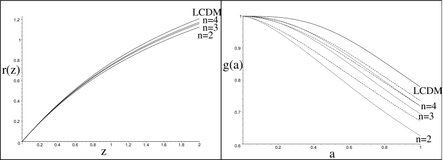
Figure 2: In the left panel, the expansion histories $r(z)=\int^{z}_{0}dzH(z)^{-1}$ are shown for LCDM, $n=4$, $n=3$ and $n=2$ from top to bottom. In the right panel, the growth factor $g(a)=\bigtriangleup(a)/a$ is shown. The solid lines are LCDM, DGP-like models for $n=4$, $n=3$ and $n=2$ from top to bottom and the dotted lines show corresponding dark energy models with the identical expansion histories

The linear growth factor is the basis for tests of modified gravity against structure formation observations. But one also needs the metric perturbations KR . In the Birkoff’s law models,

$$\frac{k^{2}}{a^{2}}(\Phi+\Psi) = -\kappa_{4}^{2}(n-1)\frac{\dot{H}}{H^{2}}\frac{\alpha(Hr_{c})}{[n\alpha(Hr_{c})-1]^{2}}\rho\bigtriangleup,$$ (74)

$$\frac{k^{2}}{a^{2}}(\Phi-\Psi) = \kappa_{4}^{2}\left[\frac{n\alpha(Hr_{c})}{n\alpha(Hr_{c})-1}+(n-1)\frac{\dot{H}}{H^{2}}\frac{\alpha(Hr_{c})}{(n\alpha(Hr_{c})-1)^{2}}\right]\rho\bigtriangleup.$$ (75)

On the other hand, in the DGP-like models,

$$\frac{k^{2}}{a^{2}}(\Phi+\Psi) = -\kappa_{4}^{2}\frac{1}{3\beta}\rho\bigtriangleup,$$ (76)

$$\frac{k^{2}}{a^{2}}(\Phi-\Psi) = \kappa_{4}^{2}\rho\bigtriangleup.$$ (77)

Equations (75) and (77) basically determine the integrated Sachs-Wolfe (ISW) and weak lensing effects. In the Birkoff’s law model, this equation receives an additional correction from the modified gravity compared with general relativity birkoff . Thus the growth factor is not enough to predict the ISW effects and weak lensing effects. Fig. 3 shows $k^{2}(\Phi-\Psi)/a^{2}\kappa_{4}^{2}\rho\bigtriangleup$. Although for $n>2$, the growth factor is almost identical in both models, the ISW effects and weak lensing effects are different due to the time variation of the functions in Eq. (75) in the Birkoff’s law model. This manifests the need for full solutions for the metric perturbations in order to predict structure formation in modified gravity models.

Figure 3: $k^{2}(\Phi-\Psi)/a^{2}\kappa_{4}^{2}\rho\bigtriangleup$ is shown for $n=2$, $n=3$, $n=4$ in the Birkoff’s law models. $k^{2}(\Phi-\Psi)/a^{2}\kappa_{4}^{2}\rho\bigtriangleup=1$ in the DGP-like models and dark energy models in general relativity.

VI conclusion

In this paper, we studied structure formation in phenomenological models in which the modified Friedmann equaiton is given by Eq. (18). In order to study the perturbations around this modified background, we constructed simple covariant equations which reproduce the modified Friedmann equation in the cosmological background. By requiring that the Bianchi identity is satisfied, a possible form of the effective equations is restricted. At a perturbative level, we have to introduce an unknown term $E_{\mu\nu}$ in the effective equations to satisfy the Bianchi identity. The Bianchi identity imposes the constraint equations for $E_{\mu\nu}$, but they are not closed. Thus the structure of the modified theory of gravity is encoded in the additional conditions on $E_{\mu\nu}$, which are needed to close the effective equations.

In this paper, we analyze the quasi-static sub-horizon perturbations relevant for structure formation. We consider two possibilities. One is a model in which Birkoff’s law is respected and the other is a model in which the perturbations can be described by scalar-tensor gravity as in the DGP model. These models are realized by particular choices of the equation of state for $E_{\mu\nu}$. We demonstrate how the growth factor depends on the assumed structure of the modified gravity. Interestingly, in models with $n>2$, the two models give almost identical growth factor. However, this does not imply the observational consequences are the same. The growth factor is determined by the solutions for $\Psi$, but the ISW and weak lensing effects are determined by the combination $\Phi-\Psi$. We find that the two models predict different behaviours of $\Phi-\Psi$. This manifests the need for knowledge of metric perturbations in order to address structure formation in modified gravity models $-$ the parameterization of the growth factor is not enough.

In this paper, we only consider linear perturbations. It is crucial to study non-linear perturbations since the solar system constraints require that the theory must be close to general relativity at solar system scales. In the Birkoff’s law model, it is shown that below the scale $r_{*}=(r_{g}/H_{0}^{2})^{1/3}$, the deviation from general relativity is small and the solar system constraints can be evaded birkoff . This is also true in the DGP model nonlinear . Thus we suspect the non-linear recovery of general relativity is quite generic in these phenomenological models. Detailed features of the transition from modified gravity to general relativity depend on the structure of the modified theory of gravity. If we can extract an information on the transition from linear theory to non-linear theory from observations such as weak lensing and cluster mass function, this also provides an interesting probe of the structure of the modified gravity. The effective equations are valid for non-linear physics, but we have to generalize the conditions on $E_{\mu\nu}$ to non-linear physics. It would be interesting to study the non-linear dynamics such as a spherical collapse based on the effective equations and we will leave this issue as a future work.

The obvious outstanding issue is to find a fundamental theory that reproduces the effective equations in this paper. Only the underlying theoretical model is capable of fixing unambiguously the conditions for $E_{\mu\nu}$ and hence the growth rate . Moreover, in a self-accelerating universe in the DGP model, the additional suppression of the growth rate compared with a dark energy model is tightly connected with the pathology of the model. In this model, the scalar mode of the graviton behaves like a ghost. This is the origin of the additional suppression of the growth rate, because the ghost gives a repulsive force and this prevents the CDM over-density from collapsing. Our analysis may indicate a possibility of avoiding the ghost by changing the boundary condition for $E_{\mu\nu}$, because the conclusion of having a theory with a negative BD parameter comes from a specific condition on $E_{\mu\nu}$ based on regularity in the bulk. This modification may be achieved by an introduction of a second brane in the bulk tanaka . The growth rate is sensitive to this modification. Hence it is crucial to develop a consistent theory for the modified gravity and, once we have a consistent theory, structure formation measures become essential to test the theory against observations.

Acknowledgments: We would like to thank R. Maartens for discussions and a careful reading of this manuscript. KK is supported by PPARC.

Appendix A Construction of covariant tensor ${}^{(n)}\Pi_{\mu\nu}$

In this appendix, we construct an expressions for ${}^{(n)}\Pi_{\mu\nu}$. We first construct ${}^{(n)}\Pi_{\mu\nu}$ as a function of $T_{\mu\nu}$ and then replace $T_{\mu\nu}$ by $\tilde{T}_{\mu\nu}$. We start from the simplest case where ${}^{(n)}\Pi_{\mu\nu}$ is a quadratic function of the energy-momentum tensor $T_{\mu\nu}$. In this case the answer is known from the effective equations in the DGP model, i.e. Eq. (6), but it is instructive to reconstruct this expression. The general form of ${}^{(2)}\Pi_{\mu\nu}$ is given by

$${}^{(2)}\Pi^{\mu}_{\>\>\nu}=A_{1}T_{\mu\alpha}T^{\alpha}_{\>\>\nu}+A_{2}TT^{\mu}_{\>\>\nu}+A_{3}T_{\alpha\beta}T^{\alpha\beta}\delta^{\mu}_{\>\>\nu}+A_{4}T^{2}\delta^{\mu}_{\>\>\nu},$$ (78)

where $T=T^{\alpha}_{\>\>\alpha}$. In the homogeneous and isotropic universe, we require that ${}^{(2)}\Pi^{0}_{\>\>0}\propto\rho^{2}$ and ${}^{(2)}\Pi_{\mu\nu}$ satisfies

$$\nabla^{\nu}{}^{(2)}\Pi_{\mu\nu}=0.$$ (79)

Then ${}^{(2)}\Pi_{\mu\nu}$ must be of the form

$${}^{(2)}\Pi^{\mu}_{\>\>\nu}=\left(\begin{array}[]{cc}B_{1}\rho^{2}&0\\ 0&(B_{2}\rho^{2}+B_{3}P\rho)\delta^{i}_{\>\>j}\\ \end{array}\right).$$ (80)

This requirement is sufficient to determine the coefficients $A_{1},A_{2},A_{3}$ and $A_{4}$ up to an overall normalization;

$$A_{1}=6A_{4},\quad A_{2}=-2A_{4},\quad A_{3}=-3A_{4}.$$ (81)

Then ${}^{(2)}\Pi_{\mu\nu}$ is given by

$${}^{(2)}\Pi^{\mu}_{\>\>\nu}=C_{2}\left(\begin{array}[]{cc}-\rho^{2}&0\\ 0&(\rho^{2}+2P\rho)\delta^{i}_{\>\>j}\\ \end{array}\right),$$ (82)

where $C_{2}=-2A_{4}$. Interestingly, the Bianchi identity $\nabla^{\mu}{}^{(2)}\Pi_{\mu 0}=0$ is automatically satisfied.

For $n=3$, the general form of ${}^{(3)}\Pi_{\mu\nu}$ is given by

$${}^{(3)}\Pi^{\mu}_{\nu}=A_{1}T^{\mu}_{\alpha}T^{\alpha}_{\beta}T^{\beta}_{\nu}+A_{2}T^{\alpha}_{\beta}T^{\beta}_{\alpha}T^{\mu}_{\nu}+A_{3}TT^{\mu}_{\alpha}T^{\alpha}_{\nu}+A_{4}T^{2}T^{\mu}_{\nu}+A_{5}T^{\alpha}_{\beta}T^{\beta}_{\gamma}T^{\gamma}_{\alpha}\delta^{\mu}_{\nu}+A_{6}TT^{\alpha}_{\beta}T^{\beta}_{\alpha}\delta^{\mu}_{\nu}+A_{7}T^{3}\delta^{\mu}_{\nu}.$$ (83)

The same requirement as Eq. (80) fixes the parameters as

$$A_{1}=6A_{2}-54A_{7},\;\;A_{3}=9A_{7},\;\;A_{4}=-A_{2}+3A_{7},\;\;A_{5}=-6A_{2}+45A_{7},\;\;A_{6}=2A_{2}-18A_{7}.$$ (84)

Then ${}^{(3)}\Pi^{\mu}_{\nu}$ is determined by

$$\Pi^{\mu}_{\>\>\nu}=C\left(\begin{array}[]{cc}-\rho^{3}&0\\ 0&(2\rho^{3}+3P\rho^{2})\delta^{i}_{\>\>j}\\ \end{array}\right),$$ (85)

where $C=2A_{2}-14A_{7}$. Again the Bianchi identity is automatically satisfied. Now let us consider the perturbations. Non-trivial components are calculated as

$$\delta{}^{(3)}\Pi^{0}_{\>\>i} = (6A_{2}-42A_{7})\rho^{2}\delta q_{,i},$$

$$\delta{}^{(3)}\Pi^{i}_{TT\;j} = \Big{[}(12A_{2}-81A_{7})P^{2}+(6A_{2}-36A_{7})\rho P+3A_{7}\rho^{2}\Big{]}\delta\pi^{i}_{\>\>j},$$ (86)

where $\delta{}^{(3)}\Pi^{i}_{TT\;j}$ is the transverse-traceless part of the $(i,j)$ component. In the main text, we demanded that

$$12A_{2}-81A_{7}=0.$$ (87)

This completely fixes all components except for an overall normalization and we can verify the formula Eq (38).

We can continue the same procedure for general $n$. We have checked the case for $n=4$ and $n=5$. We do not explicitly show the results because the formula is very lengthy. For $n=4$, there are $12$ coefficients in the general form and for $n=5$, there are $19$ coefficients. In all cases, a requirement similar to (80) is sufficient to determine the form of ${}^{(n)}\Pi_{\mu\nu}$ as

$${}^{(n)}\Pi^{\mu}_{\>\>\nu}=C_{n}\left(\begin{array}[]{cc}-\rho^{n}&0\\ 0&\Big{[}(n-1)\rho^{n}+nP\rho^{n-1}\Big{]}\delta^{i}_{\>\>j}\\ \end{array}\right).$$ (88)

The Bianchi identity $\nabla^{\mu}{}^{(n)}\Pi_{\mu 0}=0$ is automatically satisfied. Then we can compute the perturbations and get

$$\delta{}^{(n)}\Pi^{0}_{\>\>i} = nC_{n}\rho^{n-1}\delta q_{,i},$$

$$\delta{}^{(n)}\Pi^{i}_{TT\>j} = f_{n}(\rho,P)\delta\pi^{i}_{\>\>j}.$$ (89)

In this paper, we impose the constraint that

$$f_{n}(\rho,P)=b_{1}\rho^{n-1}+b_{2}\rho^{n-2}P.$$ (90)

This gives $n-1$ conditions. We checked that, for $n=4$ and $n=5$, these conditions can be imposed consistently and we get

$$f_{4}(\rho,P)=-C_{4}(14\rho^{3}+18\rho P),\quad f_{5}(\rho,P)=-C_{5}(25\rho^{4}+30\rho^{3}P).$$ (91)

These results can be summarized as

$$f_{n}(\rho,P)=C_{n}\left[n\left(-\frac{3}{2}n+\frac{5}{2}\right)\rho^{n-1}-\frac{3}{2}n(n-1)\rho^{n-2}P\right].$$ (92)

References

• (1) S. Perlmutter et. al., Astrophys. J. 517 565 (1999) .
• (2) see for example S. M. Carroll, V. Duvvuri, M. Trodden and M. S. Turner, Phys. Rev. D70 043528 (2004); K. Freese and M. Lewis, Phys. Lett. B 540 1 (2002).
• (3) G. R. Dvali, G. Gabadadze and M. Porrati, Phys. Lett. B 484, 112 (2000) [arXiv:hep-th/0002190].
• (4) C. Deffayet, Phys. Lett. B 502, 199 (2001) [arXiv:hep-th/0010186].
• (5) C. Deffayet, S. J. Landau, J. Raux, M. Zaldarriaga and P. Astier, Phys. Rev. D 66, 024019 (2002) [arXiv:astro-ph/0201164].
• (6) V. A. Rubakov, arXiv:hep-th/0303125; M. A. Luty, M. Porrati and R. Rattazzi, JHEP 0309 (2003) 029 [arXiv:hep-th/0303116].
• (7) A. Nicolis and R. Rattazzi, JHEP 0406 059 (2004) [arXiv:hep-th/0404159]; K. Koyama, Phys. Rev. D 72 123511 (2005) [arXiv:hep-th/0503191]; D. Gorbunov, K. Koyama and S. Sibiryakov, arXiv:hep-th/0512097.
• (8) A. Lue, R. Scoccimarro and G. D. Starkman, Phys. Rev. D 69, 124015 (2004) [arXiv:astro-ph/0401515]. See also A. Lue, arXiv:astro-ph/0510068;
• (9) M. Fairbairn and A. Goobar, arXiv:astro-ph/0511029.
• (10) U. Alam and V. Sahni, arXiv:astro-ph/0511473.
• (11) G. Dvali and M. S. Turner, arXiv:astro-ph/0301510.
• (12) T. Shiromizu, K. i. Maeda and M. Sasaki, Phys. Rev. D 62, 024012 (2000) [arXiv:gr-qc/9910076].
• (13) K. i. Maeda, S. Mizuno and T. Torii, Phys. Rev. D 68, 024033 (2003) [arXiv:gr-qc/0303039].
• (14) A. Lue, R. Scoccimarro and G. Starkman, Phys. Rev. D 69, 044005 (2004) [arXiv:astro-ph/0307034].
• (15) K. Koyama and R. Maartens, JCAP in press [arXiv:astro-ph/0511634].
• (16) E. V. Linder, Phys. Rev. D 72, 043529 (2005) [arXiv:astro-ph/0507263].
• (17) Y. S. Song, Phys. Rev. D 71, 024026 (2005) [arXiv:astro-ph/0407489]; L. Knox, Y. S. Song and J. A. Tyson, arXiv:astro-ph/0503644; M. Ishak, A. Upadhye and D. N. Spergel, arXiv:astro-ph/0507184; I. Sawicki and S. M. Carroll, arXiv:astro-ph/0510364.
• (18) C. Deffayet, G. R. Dvali, G. Gabadadze and A. I. Vainshtein, Phys. Rev. D 65 044026 (2002) [arXiv:hep-th/0106001]; A. Lue, Phys. Rev. D 66 043509 (2002) [arXiv:hep-th/0111168]; A. Gruzinov, New Astron.  10 311 (2005) [arXiv:astro-ph/0112246]; T. Tanaka, Phys. Rev. D 69 024001 (2004) [arXiv:gr-qc/0305031].
• (19) T. Tanaka, private communication.