Abstract

Gamma ray bursts are excellent candidates to constrain physical models which break the Lorentz symmetry. We consider deformed dispersion relations which break boost invariance and lead to an energy-dependent speed of light. In these models, simultaneously emitted photons from cosmological sources reach Earth with a spectral time delay that depends on the symmetry breaking scale. We estimate the possible bounds which can be obtained by comparing the spectral time delays with the time resolution of available telescopes. We discuss the best strategy to reach the strongest bounds. We compute the probability of detecting bursts that improve the current bounds. The results are encouraging, depending on the model, it is possible to build a detector that within several years will improve the present limits of 0.015 $m_{pl}$.

1 Introduction

One of the open questions of high energy physics is how to unify gravity with quantum physics. A lot of effort has been devoted to develop a theory of quantum gravity. This theory is likely to require a drastic modification of our current understanding of the space-time. At present there are two formal mathematical approaches : loop quantum gravity and superstring theory. Whatever might be the right description of the space-time at very short scales, there are some likely physical manifestations. It has been suggested, for instance, that such a theory would break what we believe to be basic symmetries of nature. In [1, 2], it was shown that Einstein Lagrangian allows for large fluctuations of the metric and the topology of the space-time on scales of order of the Planck length, creating a foam-like structure at these scales. It has been proposed that the propagation of particles in a foamy space-time is strongly affected on short scales. The medium responds differently depending on the energy of the particle, in analogy with the propagation through a conventional electromagnetic plasma [3, 4]. Thus space-time might exhibit a non-trivial dispersion relation in vacuum, violating therefore Lorentz invariance.

There are many different ways of breaking Lorentz symmetry; a background tensor field, like a magnetic field, breaks the vacuum rotational invariance, for instance. However, it has been shown that there are 46 different ways in which the standard model Lagrangian can be modified while remaining renormalizable, invariant under $SU(3)\times SU(2)\times U(1)$ and rotationally and translationally invariant in a preferred frame [5]. Among other effects, these terms cause the velocity of light to differ from the maximum attainable velocity of a particle, therefore changing the kinematics of particle decays. Modifying the dispersion relations of photons and electrons allows for new QED vertex interactions like photon splitting in vacuum, vacuum Čerenkov effect for electrons, photon decay, electron-positron annihilation to a single photon, etc. [6, 7].

In this work we consider only rotationally invariant deformations of the photon dispersion relation which produce an energy-dependent speed of light. If this effect is present in nature, it has to be absent below some energy scale, $\xi\,m_{pl}$, (where $m_{pl}$ is the Planck energy and $\xi$ a dimensionless constant), high enough to have been undetected so far. Traditionally this energy is believed to be the Planck energy which, at first, seems to make hopeless any experimental attempt to test these models. However, in 1997 Amelino-Camelia et al. [8] suggested that such models can be explored by studying the propagation of photons emitted from a distance source like a gamma ray burst (GRB) GRBs are short and intense pulses of soft gamma rays that arrive from cosmological distances from random directions in the sky. The bursts last from a fraction of a second to several hundred seconds. Most GRBs are narrowly beamed with typical energies around $10^{51}$ ergs, making them comparable to supernovae (for a recent review see [9, 10]). Because of the large distances traveled by the photons, these bursts are valuable tools to explore energies far beyond the reach of any laboratory on Earth.

If one considers photons with energies much smaller than the symmetry breaking scale, it is possible to expand the dispersion relation in powers of $E/\xi m_{pl}$. The first correction produces a tiny departure from the Lorentz invariant (LI) equations and we expect that the low energy limit of the deformed dispersion relation can be written generically as:

$$E^{2}-p^{2}c^{2}\simeq\epsilon\,E^{2}\left({E\over\xi m_{pl}}\right)^{n},$$ (1)

where $\epsilon=\pm 1$ takes into account the possibility of having either infraluminal or superluminal motion, the latter appearing in some models of quantum loop gravity [11, 12]. Photons simultaneously emitted from a GRB with different energies will travel at different speeds, and therefore will show on Earth a time delay. The goal of this paper is to explore these high energy Lorentz violation models by studying such time delays. We analyze the potential of detecting observational consequences of a modified dispersion relation like Eq. 1.

The paper is organized as follows; in section 2 we review cosmological photon propagation in the LI theory and show how these results are modified when a non LI term is introduced. We compute the travel time of cosmological photons and, as a check, compare it with the travel time obtained in the Newtonian approximation. In section 3 we turn to the observations and show how such models can be tested using GRB observations. We compare our method with previous works in section 5 and finally conclude in section 6.

2 Propagation of the photons

We consider first the propagation of a particle in a FRW universe, described by the metric $ds^{2}=-c^{2}\,dt^{2}+a(t)^{2}d\vec{x}^{2}$. The Hamiltonian of a relativistic particle is

$${\cal H}=\sqrt{m^{2}\,c^{4}+{p^{2}\,c^{2}\over a^{2}}}\;,$$ (2)

where $p$ is the comoving momentum and $m$ the mass. The Hamiltonian depends explicitly on $t$ through $a(t)$, expressing the fact that the momentum is redshifted due to the cosmological expansion. The trajectory of the particle is

$$x(t,p)=\int{p\,c^{2}\over a^{2}}{dt\over\sqrt{m^{2}\,c^{4}+{p^{2}\,c^{2}\over a^{2}}}}\;\;\;,\;\;\;p=\mbox{constant}\;.$$ (3)

For a massless particle, like a photon, Eq. 3 becomes

$$a\,\dot{x}=c\;.$$ (4)

Hence the speed of photons is an universal constant, $c$, which does not depend on the energy.

When Lorentz symmetry is broken this result is modified. As long as a theory of quantum gravity is not available, the high energy corrections to the Hamiltonian defined in Eq. 2 cannot be calculated. Here we will adopt a phenomenological approach, assuming that the Hamiltonian at high energy is an unknown function of the momentum, which reduces at low energies to Eq. 2. At small energies compared to the symmetry breaking scale, $E\ll\xi\,m_{pl}$, a series expansion is applicable. We will consider the first order correction to the LI theory.

We consider models which break boost invariance but keep rotational and translational invariance. Inspired by Eq. 2 we therefore postulate

$${\cal H}=\left[m^{2}c^{4}+{p^{2}c^{2}\over a^{2}}\left(1+\left({p\,c\over\xi m_{pl}\,a}\right)^{n}\right)\right]^{1/2},\;\;\;n=1,2,...\;\;\;.$$ (5)

Note that given Eq. 1 there is some arbitrariness in the choice of Eq. 5 concerning the $a^{-n}$ factor. We believe that this choice is physically the best motivated because any $p$ dependence should be redshifted due to the cosmic expansion.

We define the parameter $\mu$ as the ratio between the energy of the photon and the Planck energy,

$$\mu(a,p)={p\,c\over m_{pl}\,a}\;.$$ (6)

From Eq. 5 we deduce the new trajectory of a particle

$$x(t,p) \simeq \int_{t_{i}}^{t}\frac{p\,c^{2}}{a^{2}\sqrt{m^{2}c^{4}+{p^{2}c^{2}\over a^{2}}}}\left[1+{1\over 2}\,\mu^{n}\,\xi^{-n}\left(1+n+{m^{2}c^{4}\over m^{2}c^{4}+{p^{2}c^{2}\over a^{2}}}\right)\right]dt\;,$$

$$p = \mbox{constant}\;.$$ (7)

We made a linear expansion with respect to $\mu^{n}$ since Eq. 5 is only valid to linear order. The linear approximation used in equation 5 remains valid for $\mu<1$. Notice that in the limit when the symmetry breaking scale goes to infinity, $\xi\rightarrow\infty$, we recover Eq. 3 and the Lorentz symmetry is restored.

The main and striking difference with respect to the LI theory is that the speed of a massless particle depends on its momentum

$$a\,\dot{x}=c(1+{1\over 2}(1+n)\,\mu(a,p)^{n}\,\xi^{-n})\;.$$ (8)

2.1 Time delay

Because of the energy dependence of the speed of light in Eq. 8, two photons emitted at the same time from the same source with momenta $p_{1}$ and $p_{2}$, will reach Earth at times $t_{1}$ and $t_{2}$. The comoving distance traveled by both photons is the same

$$x(t_{1},p_{1}) = x(t_{2},p_{2})\;,$$ (9)

$$t_{2} = t_{1}+\Delta t\;.$$

Rewriting equation 7 in terms of the redshift and particularizing for photons, $m=0$, one obtains

$$x(z,p)={c\over H_{0}}\int_{0}^{z}\left(1+{1+n\over 2}\,\mu_{0}(p)^{n}\,\xi^{-n}\,(1+z)^{n}\right){dz\over\sqrt{\Omega_{m}(1+z)^{3}+\Omega_{\Lambda}}}\;,$$ (10)

where the cosmological parameters $H_{0}$, $\Omega_{m}$ and $\Omega_{\Lambda}$ are evaluated today [16] and we set $a_{0}=1$. Notice that

$$\mu(a,p)=\mu_{0}(p)\,(1+z)\;\;,\;\;\mu_{0}(p)\equiv\mu(a_{0},p)\;.$$ (11)

When $\xi\rightarrow\infty$, Eq. 10 becomes the standard definition of the cosmological distance, as it should.

Expanding Eq. 9 for small $\Delta t$, we obtain the time delay between two photons with momenta $p_{1}$ and $p_{2}$,

$$\Delta t_{\mbox{{\scriptsize del}}}\simeq{1+n\over 2H_{0}\,\xi^{n}}\,\Delta\mu^{n}\,{\sqrt{\Omega_{m}(1+z)^{3}+\Omega_{\Lambda}}\over\sqrt{\Omega_{m}+\Omega_{\Lambda}}}\int_{0}^{z}{(1+z)^{n}dz\over\sqrt{\Omega_{m}(1+z)^{3}+\Omega_{\Lambda}}}\;,$$ (12)

where $\Delta\mu^{n}=\mu_{0}^{n}(p_{2})-\mu_{0}^{n}(p_{1})$. Fig. 1 depicts the time delay as a function of the redshift and the momentum of the photon.

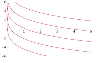
Figure 1: Curves of constant time delay as a tunction of the redshift of the source and the energy of the photon. In all the curves $n=1$ and $\xi=1$.

2.2 Newtonian approximation

It is instructive to compare the former results with those obtained in the Newtonian approximation. For small redshifts one can neglect the expansion of the universe and suppose that energy of the photons is constant. The delay between a low energy photon traveling at the standard speed of light $c$ and the a high energy photon traveling at the modified speed of light $v$ is

$$\Delta t\sim{d\over c}-{d\over v}\;,$$ (13)

where $v={dE/dp}$. In this approximation a linear relation between distance and redshift holds

$$d\simeq{c\over H_{0}}{z\over\sqrt{\Omega_{m}+\Omega_{\Lambda}}}\;.$$ (14)

Hence the time delay is

$$\Delta t\sim{1+n\over 2H_{0}}\,{z\over\sqrt{\Omega_{m}+\Omega_{\Lambda}}}\,\mu_{0}^{n}\,\xi^{-n}\;.$$ (15)

Comparing Eq. 15 and Eq. 12 we verify that the Newtonian analysis agrees to first order with its relativistic counterpart, Eq. 12.

3 Observational Detection of Lorentz Violation

To obtain an experimental bound on the symmetry breaking scale $\xi$, we need to compare the delay produced by the modified speed of light, Eq. 8, with the time resolution of the observing telescope. For a successful detection of a Lorentz violation, the delay has to be larger than the time resolution of the telescope:

$$\Delta t_{\mbox{{\scriptsize del}}}>\Delta t_{\mbox{{\scriptsize res}}}\;.$$ (16)

3.1 Telescope time resolution

The time resolution of a telescope depends on two factors. The first is the intrinsic detector minimal time resolution, $\Delta t_{\mbox{{\scriptsize detector}}}$, which is typically of order $10^{-3}-10^{-4}$s. The second factor, $\Delta t_{\mbox{{\scriptsize res}}}$, is inversely proportional to the photon detection rate which, in turn, depends on the detector effective area and on the luminosity, spectrum and distance of the source,

$$\Delta t_{\mbox{{\scriptsize res}}}\simeq{b\over A\,P_{\gamma}(E_{1},E_{2})}\;.$$ (17)

where $P_{\gamma}(E_{1},E_{2})$ is the photon peak flux in the energy band $(E_{1},E_{2})$ and $A$ is the detector effective area. The factor $b$ takes into account the minimum number of photons needed to resolve a peak. If the noise of the detector is negligible, $b$ is of order 5-10. In the following examples we consider an idealized detector with no noise and set $b=6$.

The overall time resolution is given by

$$\tilde{\Delta t_{\mbox{{\scriptsize res}}}}=\max(\Delta t_{\mbox{{\scriptsize res}}},\Delta t_{\mbox{{\scriptsize detector}}})\;.$$ (18)

The photon flux depends on the energy interval and therefore it is sensitive to the spectrum of the burst. A good phenomenological fit for the high energy GRB photon spectrum is

$$N({\cal E})=R_{1}\,{\cal E}^{-\beta}\;,$$ (19)

where ${\cal E}$ is the energy in the rest frame of the burst, and $N({\cal E})$ has units of photons keV^-1 s^-1. This fit is valid for energies higher than ${\cal E}_{0}$, where ${\cal E}_{0}$ is typically of order of a few hundred keV. In what follows, we will take ${\cal E}_{0}\sim$ 100 keV. For this spectrum the flux in the energy band $(E_{1},E_{2})$ is

$$P_{\gamma}(E_{1},E_{2})={1\over 4\pi d(z)^{2}}\,{R_{1}\over 1+z}\int^{E_{2}(1+z)}_{E_{1}(1+z)}{\cal E}^{-\beta}\,d{\cal E}.$$ (20)

The factors $(1+z)$ in the limits of the integral transform rest-frame energies into Earth measured energies, and there is an extra $(1+z)$ because of the cosmological time dilation; $d(z)$ is the cosmological distance.

Let us introduce the (isotropic equivalent) peak luminosity in the GRB rest frame is

$${\cal L}_{peak}=R_{1}\int^{\infty}_{{\cal E}_{0}}{\cal E}^{-\beta}\,{\cal E}\,d{\cal E}.$$ (21)

Combining Eq. 20 and Eq. 21 we obtain

$$\Delta t_{\mbox{{\scriptsize res}}}=b\,{4\pi d(z)^{2}\over A}\,{\beta-1\over\beta-2}\,{(1+z)^{\beta}\over{\cal L}_{peak}}\,{{\cal E}_{0}^{2-\beta}\over E_{1}^{1-\beta}-E_{2}^{1-\beta}}\;,$$ (22)

In the following sections we will also need to estimate the resolution from the photon energy flux $P(E_{1},E_{2})$ and from the luminosity of the bursts. Using

$$P(E_{1},E_{2})={R_{1}\over 4\pi d(z)^{2}\,(1+z)}\,\int^{E_{2}(1+z)}_{E_{1}(1+z)}{\cal E}^{-\beta}\,{\cal E}\,d{\cal E}\;,$$ (23)

the time resolution is obtained by combining Eq. 20, 22 and 23,

$$\Delta t_{\mbox{{\scriptsize res}}}\simeq{b\over A\,P(E_{1},E_{2})}\,{\beta-1\over\beta-2}\,(1+z)\,{E_{2}^{2-\beta}-E_{1}^{2-\beta}\over E_{2}^{1-\beta}-E_{1}^{1-\beta}}\;.$$ (24)

3.2 A bound on $\xi$

Comparing Eq. 12 and 22 we find that we can test symmetry breaking scales up to:

$$\xi^{n}<{AH_{0}\over 8\pi\,b\,c^{2}}\,{\beta-2\over\beta-1}\,{\cal E}_{0}^{\beta-2}\,{\cal L}_{peak}\,\left(1-\left(E_{2}\over E_{1}\right)^{1-\beta}\right)\,{\Delta\mu^{n}\over E_{1}^{\beta-1}}\,\,{\cal G}_{n}(z)\;,$$ (25)

where all the redshift dependence is contained in the function ${\cal G}_{n}(z)$ (remember that ${\cal L}_{peak}$ is defined in the rest frame of the burst).

For distant bursts, the limiting resolution is determined by the photon arrival rate and therefore $\tilde{\Delta t_{\mbox{{\scriptsize res}}}}=\Delta t_{\mbox{{\scriptsize res}}}$. In this case, the function ${\cal G}_{n}(z)$ is given by:

$${\cal G}_{n}(z) = (1+n){\sqrt{\Omega_{m}(1+z)^{3}+\Omega_{\Lambda}}\over\sqrt{\Omega_{m}+\Omega_{\Lambda}}}\,\int_{0}^{z_{0}}{(1+z)^{n}dz\over\sqrt{\Omega_{m}(1+z)^{3}+\Omega_{\Lambda}}}$$ (26)

$$\cdot\left(\int^{z}_{0}{dz\over\sqrt{\Omega_{m}\,(1+z)^{3}+\Omega_{\Lambda}}}\right)^{-2}\,(1+z)^{-\beta}\;.$$

On the other hand, for nearby bursts $\tilde{\Delta t_{\mbox{{\scriptsize res}}}}$ is limited by the detector resolution. Fig. 2 depicts the behavior of ${\cal G}_{n}(z)$. For small redshifts, ${\cal G}_{n}(z)$ increases from zero up to a maximum value where $\Delta t_{\mbox{{\scriptsize detector}}}=\Delta t_{\mbox{{\scriptsize res}}}$. ${\cal G}_{n}(z)$ is shown in this regime for $\Delta t_{\mbox{{\scriptsize detector}}}=10^{-4}$ s (upper branch) and $10^{-3}$ s (lower branch). For higher redshifts, $\tilde{\Delta t_{\mbox{{\scriptsize res}}}}$ is dominated by $\Delta t_{\mbox{{\scriptsize res}}}$. The function ${\cal G}_{n}(z)$ decreases then up to a minimum and finally increases again at high redshift (for $n=1$ the growth begins at $z>5$, which is too large to be experimentally interesting). As the limit on $\xi$ is proportional to ${\cal G}_{n}^{1/n}(z)$ the best limit is obtained at small redshifts, when $\Delta t_{\mbox{{\scriptsize res}}}=\Delta t_{\mbox{{\scriptsize detector}}}$.

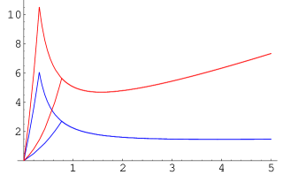
Figure 2: ${\cal G}_{n}(z)$ as a function of the redshift for $\beta=2.5$. For small redshifts ${\cal G}_{n}(z)$ has two branches, the upper one corresponds to $\Delta t_{\mbox{{\scriptsize detector}}}=10^{-4}$ s and the lower one corresponds to $\Delta t_{\mbox{{\scriptsize detector}}}=10^{-3}$ s.

This is a non intuitive result. One would expect that the best bound on $\xi$ is obtained from photons arriving from bursts at very high redshifts, which have significant larger delays than photons from nearby bursts. However the distance also dilutes the photons decreasing the time resolution. Moreover, due to the redshift of the energy, a fixed energy band on Earth corresponds to an intrinsically higher energy band which is more scarce in photons. These two combined effects overcome the improvement of the bound due to the larger delay. Thus, to obtain the tightest bound it is preferable to use low redshift bursts. As it can be seen in Fig. 2, low redshift means here $z<1$ (but this depends, of course, on the intrinsic detector resolution). Note that we have not yet taken into account the possible attenuation of the interstellar medium. This result is merely based on geometric considerations.

Let us turn our attention to the influence of the energy range in which we observe the burst. If we observe photons in the interval $(E_{1},E_{2})$, $\mu^{n}$ satisfies

$$\mu^{n}>\left(E_{1}\over m_{pl}\right)^{n}\;,$$ (27)

and the energy dependence in Eq. 25 is bounded by

$$E_{1}^{\,\,n+1-\beta}\,\left(1-\left(E_{2}\over E_{1}\right)^{1-\beta}\,\right)\;.$$ (28)

The exponent $n+1-\beta$ is positive for $n>\beta-1$. The parameter $\beta$ can vary between $1.6<\beta<5$ [23] (the lower limit of $\beta\sim 5$ corresponds, however, to bursts which do not have a high energy tail and are consequently not interesting for our purposes). For typical bursts $\beta\sim 2.5$. For $n\geq 2$ and $\beta\sim 2.5$ the exponent $n+1-\beta$ is positive and therefore the best bound is obtained by observing in the highest possible energy band. On the contrary, for $n=1$ and $\beta\sim 2.5$ the exponent is negative and it is advantageous to use the low energy bands. Note that this analysis is based on the assumption that the spectrum is given by Eq. 19, which is valid for energies higher than ${\cal E}_{0}$. We should therefore always observe at energies higher than ${\cal E}_{0}$.

Like the discussion about the optimal redshift, this is another non intuitive result. Contrary to what would be naively expected, we have shown that the optimal energy range is not necessarily the highest one, but depends on the model of symmetry breaking and on the burst spectrum. These results apply only for a given detector with a fixed collecting area. Observations in a higher energy band might be advantageous under different conditions, for instance, if they are made with a different telescope with a larger area. Finally, cosmic attenuation sets an upper limit on the energy range. We discuss this issue in the section 3.3.

From Eq. 28 is evident that the larger the ratio $E_{2}/E_{1}$, the better the bound (broadening the energy band increases the number of photons and consequently the telescope resolution); however, in order to avoid a large spread in the arrival times, the detected photons in each channel should have comparable energies.

The bound can be rewritten as

$$\xi_{n}>\sigma\left[{{\cal L}_{peak}\over{\cal L}_{*}}\,\,{\cal G}_{n}(z)\right]^{1/n}\;,$$ (29)

where

$$\sigma=\left[{AH_{0}\over 8\pi\,b\,m_{pl}^{n}\,c^{2}}\,{\beta-2\over\beta-1}\,{\cal L}_{*}\,{\cal E}_{0}^{\beta-2}\,E_{1}^{n+1-\beta}\left(1-\left(E_{2}\over E_{1}\right)^{1-\beta}\right)\right]^{1/n}\;.$$ (30)

We have introduced the quantity ${\cal L}_{*}=6.3\cdot 10^{51}$ erg s^-1, which will be useful later on when dealing with luminosity distributions. In Eq. 29 we have explicitly separated the redshift and burst luminosity and included all the numerical values and telescope dependent quantities in the constant $\sigma$,

$$\sigma\sim 10^{22{1-n-\beta\over n}}\left(\,{\beta-2\over\beta-1}\right)^{1/n}\,\left({A\over 2000\mbox{ cm}^{2}}\right)^{1/n}\,\left(E_{1}\over\mbox{MeV}\right)^{1+{1-\beta\over n}}\,\left(1-\left(E_{2}\over E_{1}\right)^{1-\beta}\right)^{1/n}.$$ (31)

We see again that for $n=1$ and $\beta>2$ going to high energies does not improve the bound.

The order of magnitude of achievable bounds for typical bursts obtained in Eq. 29 is $10^{-3}$ for $n=1$ and $3\cdot 10^{-13}$ for $n=2$ (for $\beta=2.5$ in both cases). This is in agreement with actual limits found for specific bursts in the literature. Ellis et al. [13] used a wavelet analysis to look for correlations between redshift and spectral time lags between the arrival times of flares at different energies, and obtained the bounds of $\xi_{1}>5.6\cdot 10^{-4}$ and $\xi_{2}>2.4\cdot 10^{-13}$ at a 95% of confiance level. Subsequently this result was improved [14] by using a more complete data set of transient sources with a broad spread in redshifts to correct for intrinsic time delays (we discuss intrinsic delays in section 5). A different approach was adopted by Boggs et al. [17], who considered a single and extremely bright burst, GRB 011206. This burst yielded the bounds of $\xi_{1}>0.015$ and $\xi_{2}>4.5\cdot 10^{-12}$ respectively.

3.3 Cosmic attenuation

At energies of TeV and higher, the universe becomes opaque due to the interaction of the gamma ray photons with the background light to create electron-positron pairs, $\gamma\gamma\rightarrow\mbox{e}^{-}\mbox{e}^{+}$. The cross section of this reaction is maximized when the product of the energies of both photons is $\sim(m_{e}c^{2})^{2}$. A photon of 10 TeV will interact with an infrared photon, for instance, creating an electron-positron pair.

For $n=1$ we are concerned with lower energies, from a few hundreds keV to a few MeV. A these energies we can safely neglect attenuation. Fig 3 shows the optical thickness of the extragalactic medium at 10 GeV [20]. As it can be seen, attenuation only becomes important at high redshift, $z>3$. Clearly, it is safe to ignore this effect at lower energies.

Figure 3: Optical thickness of the intergalactic medium at 10 GeV

3.4 A quantitative example : GRB 050603A

For an observed burst on Earth, we can skip Eq. 25 which depends on quantities defined in the rest frame of the burst (${\cal L}_{peak}$ and ${\cal E}_{0}$) and calculate the bound directly from the flux on Earth. The quantities usually measured are the energy flux $P(E_{1},E_{2})$ (in erg cm^-2 s^-1) or the photon flux $P_{\gamma}(E_{1},E_{2})$ (in photons cm^-2 s^-1).

GRB 050603A is a very bright burst with measured redshift $z=2.821$ observed with two satellites : Konus-Wind (area $\sim 200$ cm²) and Swift-BAT (area $\sim 5200$ cm²). The time-integrated spectrum is well fitted by a high energy photon index $\beta=2.15$. Konus measured a peak flux of $3.2\cdot 10^{-5}$ erg cm^-2 s^-1 in the (20 keV, 3 MeV) band. These values correspond to:

$\Delta t_{\mbox{{\scriptsize res}}}$ (20 keV, 3 MeV)		$\sim\;5\cdot 10^{-4}$ s
$n=1$	$\Delta t_{del}$ (20 keV)	$\sim\;9\cdot 10^{-6}/\xi\;$ s
$n=2$	$\Delta t_{del}$ (20 keV)	$\sim\;5\cdot 10^{-29}/\xi^{2}\;$ s

For the same burst Swift detected a peak flux of 31.8 photons cm^-2 s^-1 in the (15 keV, 350 keV) band. This implies

$\Delta t_{\mbox{{\scriptsize res}}}$ (15 keV, 350 keV)		$\sim\;4\cdot 10^{-5}$ s
$n=1$	$\Delta t_{del}$ (15 keV)	$\sim\;7\cdot 10^{-6}/\xi\;$ s
$n=2$	$\Delta t_{del}$ (15 keV)	$\sim\;3\cdot 10^{-29}/\xi^{2}\;$ s

If the time delays at these low energy bands were not contaminated with intrinsic spectral delays at the source, this burst could have led to the following limits:

	Konus	Swift
$n=1$	$\xi>0.02$	$\xi>0.2$
$n=2$	$\xi>3\cdot 10^{-13}$	$\xi>9\cdot 10^{-13}$

The time resolution used in this example, $4\cdot 10^{-5}$ s, is in fact below the limiting time resolution of Swift, 0.1 ms. Swift resolution would have led to a slightly weaker bound, $\xi_{1}>0.07$. Furthermore, we have considered here photons all the way down to 15 keV (Swift) or 20 keV (Konus). Limiting the discussion to photons above $\sim 100$ keV, for which Eq. 19 is accurate, would have reduced the limits further.

The numbers obtained here are clearly idealized and should serve only as an example of what can be achieved. In order to set an experimental bound, we need to observe the burst in two different energy channels and compare the arrival time in each one. An additional problem is posed by the observed intrinsic delay in the emission times of the photons at the source [13, 24] which we discuss in section 5.

4 Distribution of bursts

GRB 050603A could have given a very powerful bound on $\xi$. But how likely would it be to detect a burst yielding such a bound or a higher one ? From the results of the previous sections, the more luminous and closer the burst, the stronger the bound. In this section we estimate the probability of finding such a burst, given an empirical luminosity and space distribution of bursts.

To improve a bound, $\xi_{0}$, we need to detect a burst with a luminosity and a redshift such that

$$\sigma^{n}\,\,{{\cal L}\over{\cal L}_{*}}\,\,{\cal G}_{n}(z)>\xi_{0}^{n}\;\;.$$ (32)

Eq. 32 define a region in the luminosity and redshift space-phase (see Fig. 4). The probability for such a burst to happen is given by the integral of the probability of finding a burst over this region.

Figure 4: The luminosity and the redshift needed to give a bound of $\xi_{0}=0.2$ for $n=1$. Higher bounds are obtained above the curve.

Let us introduce the local peak luminosity function, $\Phi_{0}({\cal L})$, defined as the fraction of GRBs with luminosities in the interval $\log{\cal L}$ and $\log{\cal L}+d\log{\cal L}$, can be approximated by [18]:

$$\Phi_{0}({\cal L})=c_{0}\left\{\begin{array}[]{ll}({\cal L}/{\cal L}_{*})^{{\alpha_{1}}}&{\cal L}_{*}/\Delta_{1}<{\cal L}<{\cal L}_{*}\\ ({\cal L}/{\cal L}_{*})^{{\alpha_{2}}}&{\cal L}_{*}<{\cal L}<\Delta_{2}{\cal L}_{*}\end{array}\right.\;,$$ (33)

where $c_{0}$ is a normalization constant such that the integral over the luminosity function equals the unity.

There is a strong evidence that long GRBs follow the comoving star formation rate (SFR), $R_{SFR}(z)$. Namely, $R_{GRB}(z)$, the comoving GRB rate satisfies $R_{GRB}(z)\propto R_{SFR}(z)$. We employ the parametrization of Porciani et al. [19] for the comoving SFR distribution. From it we write

$$R_{GRB}(z)=\rho_{0}\frac{23\exp(3.4z)}{\exp(3.4z)+22}\,{\sqrt{\Omega_{m}(1+z)^{3}+\Omega_{\Lambda}}\over(1+z)^{3/2}}\;.$$ (34)

The luminosity function at redshift $z$ is therefore $\Phi(z,{\cal L})=\Phi_{0}({\cal L})\,R_{GRB}(z)$. Guetta et al. [25] used the BATSE peak flux distribution, to estimate the parameters $\rho_{0}$, $\alpha_{1}$ and $\alpha_{2}$. For long bursts they found two different fits:

	$\alpha_{1}$	$\alpha_{2}$	$\Delta_{1}$	$\Delta_{2}$	${\cal L}_{*}$ (erg s-1)	$\rho_{0}$ (Gpc-3 yr-1)
I	-0.1	-2	30	50	$6.3\cdot 10^{51}$	0.18
II	-0.6	-3	30	50	$1.6\cdot 10^{52}$	0.16

Short GRBs, which constitute about one quarter of the observed bursts, do not follow the SFR [26, 27] and will not be discussed here.

The probability of detecting a burst which sets a bound $\xi>\xi_{0}$ is

$$N(\xi>\xi_{0})=\int^{\infty}_{0}{R_{GRB}(z)\over 1+z}{dV(z)\over dz}dz\int^{\infty}_{\Lambda}\Phi_{0}({\cal L})d\log{\cal L},$$ (35)

where the factor $(1+z)^{-1}$ accounts for the cosmological time dilation and $V(z)$ is the comoving volume. The factor $\Lambda$ is defined as

$$\Lambda=\max\left({\xi_{0}^{n}\,{\cal L}_{*}\over\sigma^{n}{\cal G}_{n}(z)},{\cal L}_{min}\right),$$ (36)

where ${\cal L}_{min}$ is the minimal luminosity for a burst to be detected

$${\cal L}_{min}=4\pi\,d(z)^{2}\,(1+z)^{\beta}\,{\beta-1\over\beta-2}\,{{\cal E}_{0}^{2-\beta}\over E_{1}^{1-\beta}-E_{2}^{1-\beta}}\,{\cal N}_{min}.$$ (37)

${\cal L}_{min}$ depends on the sensitivity of the telescope, ${\cal N}_{min}$, which is the minimal photon flux necessary to trigger the instrument. We considered for $n=1$ an idealized detector, Det. I, with an area of 5200 cm² making observations in the energy band (500 keV, 2 MeV). For $n=2$, we focused on the forthcoming spatial observatory GLAST which will be launched in 2006. We considered the energy band (100 MeV, 1 GeV) where GLAST is expected to have an effective area of 8000 cm².

Integrating numerically Eq. 35 we find

	Det. I		GLAST
	$\;\;\;\;\xi_{1}$	rate (bursts yr-1)	$\xi_{2}\;\;\;\;\;\;\;$	rate (bursts yr-1)
GRB 021206	0.015	(7.4 - 6.9)$\cdot 10^{-1}$	${\bf 4.5\cdot 10^{-12}}$	9.4 - 12.8
	0.05	(2.8 - 3.1)$\cdot 10^{-1}$	$7\cdot 10^{-12}$	1.9 - 2.2
	0.1	(9.1 - 6.9)$\cdot 10^{-2}$	$10^{-11}$	(4.8 - 3.5)$\cdot 10^{-1}$
	0.5	(2.1 - 1.3)$\cdot 10^{-3}$	$2.5\cdot 10^{-11}$	(5.0 - 2.4)$\cdot 10^{-3}$
	1.0	(3.5 - 2.0)$\cdot 10^{-4}$	$5\cdot 10^{-11}$	(7.2 - 3.9)$\cdot 10^{-5}$

The values in the first row correspond to the bounds obtained from GRB 021206 [17]. To estimate ${\cal L}_{min}$, we assumed that the ideal detector, Det. I, has a sensitivity of ${\cal N}_{min}\sim$ 1 ph cm^-2 s^-1, which is comparable to the sensitivities estimated by Band [28] for several detectors in similar energy bands. For GLAST, we took ${\cal N}_{min}\sim 4\cdot 10^{-6}$ ph cm^-2 s^-1, which roughly means that the detector is very quiet at these energies and a detection of 6 photons during the whole duration of the burst ($\sim$ 3 minutes) is enough to identify it.

Finally we took into account the partial sky coverage of any real telescope to compute the number of bursts observed per year. GLAST opening angle will be $\sim$ 2 stereoradian; we used a similar opening angle for our idealized detector.

5 Comparison with other works

The idea of using GRBs to set experimental bounds on a possible violation of Lorentz symmetry was first suggested by Amelino-Camelia et al. [8]. Later on, several groups made use of it to explore these limits [13, 17, 14]. The current best bounds have been obtained by Boggs et al. [17] who used a very bright burst, GRB 021206, to set a limit on the symmetry breaking scale. The data consisted of light curves in six energy bands spanning 0.2 - 17 MeV. The redshift of this burst is not known, but an approximated redshift of $z\simeq 0.3$ was estimated from the spectral and temporal properties of the burst (this method involves, however, a very high uncertainty which can be as high as a factor of 2).

The observed fluence of GRB 021206 is $1.6\cdot 10^{-4}$ ergs cm² at the energy range of 25-100 kev [21]. This puts GRB 021206 as one of the most powerful bursts ever observed. GRB 021206 also shows a very atypical photon spectrum at the MeV range. Instead of decreasing with the energy following a power law with $\beta\sim 2.5$, it is almost flat from 1 MeV up to 17 MeV, namely $\beta\sim 0$ (this implies in particular that $F_{\nu}$ increases with $\nu$ in these energies). This flatness allows to resolve a fast flare and to determine its peak time and uncertainty in several bands. The analysis of the dispersion of these peak times yields to the lower bounds $\xi_{1}>0.015$ and $\xi_{2}>5\cdot 10^{-12}$ [17]. Applying our method on the energy band 15-350 keV using data from the GRB 050603A, we obtained a theoretical upper limit to the lower bounds of $\xi_{1}>0.2$ and $\xi_{2}>9\cdot 10^{-13}$. These numbers represent the best bounds that could be obtained if the time resolution of the detector was high enough ($\sim 5\cdot 10^{-5}$ s), the detector noise was negligible and we had at our disposal the light curves in at least two energy channels.

Our conclusions on the optimal redshift and energy band are based on a power law spectrum $E^{-\beta}$ with $\beta\geq 2$. They arise from comparing the time delay, which always increases with the energy, with the time resolution of the telescope. Comparing both energy dependencies, we found in section 3.2 that for $n=1$ and $\beta>2$ is better to observe at low energies. However if $\beta<2$, like in GRB 021206 in the MeV range, this conclusion does not hold and it is preferable to use the highest available energy band. In this case the GLAST Large Area Telescope will be a very powerful tool. It is expected to be sensitive from 20 MeV to 300 GeV with a peak effective area in the range 1-10 GeV of 8000 cm². Observing with GLAST in energy bands below 10 GeV where cosmic extinction is still negligible (see fig. 3) can improve dramatically our current bounds. At present little is known about GRB emission at energies higher than 50 MeV and therefore it is not possible to estimate how common are bursts with $\beta<2$. Taking advantage of atypical bursts to explore even higher energies is an exciting possibility to keep in mind, however at present it is difficult to design a strategy based only in these bursts.

As already mentioned, our bound must be interpreted as a theoretical one, i.e. the highest bound that could be set, were the best conditions achieved. We already commented on the necessity of observing in at least two energy channels and to take into account the real time resolution of the detector.

An additional serious problem is the intrinsic lack of simultaneity in the pulse emission in the keV regime [13, 24]. Soft emission has a time delay relative to high energy emission [22]. While the reason for this phenomenon is not understood, an anti-correlation between the spectral evolution timescale and the peak luminosity has been found [15]. There are two different ways to deal with the intrinsic delay. The first is to try to reduce it by choosing very luminous bursts and observing in MeV or higher, where the delay, if still exists, seems to be smaller. The second approach is based on the fact that the delays produced by a violation of Lorentz symmetry increase with the redshift of the source, whereas intrinsic time delays are independent of the redshift of the source [14]. Thus, a systematic comparison of a delays in a group of bursts with known redshifts could enable us to distinguish between intrinsic and redshift dependent delays. Using a sample of 35 bursts with known redshifts, Ellis et al. [14] established a lower limit of $\xi_{1}>7\cdot 10^{-4}$ on the symmetry breaking scale. These bounds are two orders of magnitude lower than our theoretical limits. This difference demonstrates the importance that intrinsic time delays, noise and the real instrumental resolution can have.

6 Conclusions

Our goal was to explore the potential of GRBs to set bounds on Lorentz violation and to find optimal techniques to do so. We modified the dispersion relation of photons by adding an extra term proportional to the photon momentum to the power $n+2$. We have shown that in models with $n=1$ it is possible to explore energies which are close to the Planck energy. When $n=2$, the energies explored are smaller, around $10^{7}$ GeV. These bounds are idealized and they do not take into account experimental limitations or the intrinsic time-structure of the $\gamma$-ray emission. They should serve as theoretical estimations of what can be achieved. The methodology we use here can be used to design future optimal experiments for observing this effect (or setting bounds on it).

We have modelled the burst high energy emission with a power law spectrum $E^{-\beta}$ with $\beta\geq 2$. This fits well the time integrated emission of most of the bursts. We found two non intuitive results: (i) The optimal redshift to set the strongest bound is less than 1. (ii) For $n=1$, low energy, rather than high energy emission is preferred. Both results are counter-intuitive since the Lorentz violation delay increases with the distance and with the energy. However, distance or observations at high energies (where the flux is lower) dilute the photons reducing the temporal resolution achieved on Earth. It turns out that this is the dominant effect.

In the models with $n=2$, going to higher energies always improves the bounds. Here the situation will be remarkably changed when the spatial observatory GLAST will become operational.

We have also investigated the probability of improving the current experimental bounds, given a phenomenological luminosity and space distribution of bursts. As we are discussing idealized bounds, this probability should only be trusted up to an order of magnitude.

References

- [1] J. A. Wheeler, Annals Phys. 2, 604 (1957).
- [2] S. W. Hawking Nucl. Phys. B 144, 349 (1978)
- [3] I. T. Drummond and S. J. Hathrell, Phys. Rev. D 22, 343 (1980).
- [4] J. I. Latorre, P. Pascual and R. Tarrach Nucl. Phys. B 437 60 (1995) [arXiv:hep-th/9408016].
- [5] S. R. Coleman and S. L. Glashow, Phys. Rev. D 59, 116008 (1999) [arXiv:hep-ph/9812418].
- [6] T. Jacobson, S. Liberati and D. Mattingly, Phys. Rev. D 67, 124011 (2003) [arXiv:hep-ph/0209264].
- [7] A. Kostelecky and M. Mewes Phys. Rev. D 66, 056005 (2002)
- [8] G. Amelino-Camelia, J. R. Ellis, N. E. Mavromatos, D. V. Nanopoulos and S. Sarkar, Nature 393, 763 (1998) [arXiv:astro-ph/9712103].
- [9] T. Piran, Rev. Mod. Phys. 76, 1143 (2004) [arXiv:astro-ph/0405503].
- [10] B. Zhang and P. Meszaros, Int. J. Mod. Phys. A 19, 2385 (2004) [arXiv:astro-ph/0311321].
- [11] R. Gambini and J. Pullin, Phys. Rev. D 59, 124021 (1999) [arXiv:gr-qc/9809038].
- [12] J. Alfaro, H. A. Morales-Tecotl and L. F. Urrutia, Phys. Rev. Lett. 84, 2318 (2000) [arXiv:gr-qc/9909079].
- [13] J. R. Ellis, N. E. Mavromatos, D. V. Nanopoulos and A. S. Sakharov, Astron. Astrophys. 402, 409 (2003) [arXiv:astro-ph/0210124].
- [14] J. Ellis, N. E. Mavromatos, D. V. Nanopoulos, A. S. Sakharov and E. K. G. Sarkisyan, [astro-ph/0510172]
- [15] J. P. Norris, G. F. Marani and J. T. Bonnell, [arXiv:astro-ph/9903233].
- [16] D. N. Spergel et al. [WMAP Collaboration], Astrophys. J. Suppl. 148, 175 (2003) [arXiv:astro-ph/0302209].
- [17] S. E. Boggs, and C. B. .Wunderer, K. Hurley and W. Coburn, Astrophys. J. 611, L77-L80 (2004) [astro-ph/0310307].
- [18] M. Schmidt, Astrophys. J. 523, L117-L120 (1999) [astro-ph/9908206].
- [19] C. Porciani and P. Madau, Astrophys. J. 548, L522-L531 (2001) [astro-ph/0008294]
- [20] J. R. Primack, J. S. Bullock and R. S. Somerville, AIP Conf. Proc. 745, 23 (2005) [arXiv:astro-ph/0502177].
- [21] K. Hurley et al., GCN Circ. 1727, 1728 (2002)
- [22] J. P. Norris, R. J. Nemiroff, J. T. Bonnell, J. D. Scargle, C. Kouveliotou, W. S. Paciesas, C. A. Meegan and G. J. Fishman, Astrophys. J. 459, L393-L531 (1996).
- [23] D. Band, J. Matteson, L. Ford, B. Schaefer, D. Palmer, B. Teegarden, T. Cline, M. Briggs, W. Paciesas, G. Pendleton, G. Fishman, C. Kouveliotou, C. Meegan, R. Wilson and P. Lestrade, Astrophys. J. 413, L281-L292 (1993).
- [24] T. Piran, “Gamma Ray Bursts as Probes of Quantum Gravity”, [arXiv:astro-ph/0407462].
- [25] D. Guetta, T. Piran and E. Waxman, Astrophys. J. 619, L412-L419 (2005) [arXiv:astro-ph/0311488].
- [26] D. Guetta, and T. Piran, Astron. & Astrophys., 435, 421, (2005)
- [27] D. Guetta, and T. Piran, submitted to Astron. & Astrophys., astro-ph/0511239, (2006)
- [28] D. L. Band, Astrophys. J. 588, 945 (2003) [arXiv:astro-ph/0212452].