Automated analysis of eclipsing binary lightcurves. I. EBAS — a new Eclipsing Binary Automated Solver with EBOP

Abstract

We present a new algorithm — Eclipsing Binary Automated Solver (EBAS), to analyse lightcurves of eclipsing binaries. The algorithm is designed to analyse large numbers of lightcurves, and is therefore based on the relatively fast EBOP code. To facilitate the search for the best solution, EBAS uses two parameter transformations. Instead of the radii of the two stellar components, EBAS uses the sum of radii and their ratio, while the inclination is transformed into the impact parameter. To replace human visual assessment, we introduce a new ’alarm’ goodness-of-fit statistic that takes into account correlation between neighbouring residuals. We perform extensive tests and simulations that show that our algorithm converges well, finds a good set of parameters and provides reasonable error estimation.

1 Introduction

The advent of large CCDs for the use of astronomical studies has driven a number of photometric surveys that have produced unprecedentedly large sets of lightcurves of eclipsing binaries (e.g., Alcock et al., 1997). The commonly used interactive way of finding the set of parameters that best fit an eclipsing binary lightcurve utilizes human guess for the starting point of the iteration, and further human decisions along the converging iteration (e.g., Ribas et al., 2000). Such a process is not always repeatable, and is impractical when it comes to the large set of lightcurves at hand.

The OGLE project, for example, yielded a huge photometric dataset of the SMC (Udalski et al., 1998) and the LMC (Udalski et al., 2000), which includes a few thousand eclipsing binary lightcurves (Wyrzykowski et al., 2003). This dataset allows for the first time a statistical analysis of the population of short-period binaries in another galaxy. A first effort in this direction was performed by North & Zahn (2003, hereafter NZ03), who derived the orbital elements and stellar parameters of 153 eclipsing binaries in the SMC in order to study the statistical dependence of the eccentricity of the binaries on their separation. In a following study, North & Zahn (2004, hereafter NZ04) analyzed another sample of 509 lightcurves selected from the 2580 eclipsing binaries discovered in the LMC by the OGLE team (Wyrzykowski et al., 2003). However, the OGLE LMC data contain many more eclipsing binary lightcurves. An automated algorithm would have made an analysis of the whole sample possible.

To meet the need for an algorithm that can handle a large number of lightcurves we developed EBAS — Eclipsing Binary Automated Solver, which is a completely automatic scheme that derives the orbital parameters of eclipsing binaries. Such an algorithm can be of use for the OGLE lightcurves, as we do in the next paper, and for the data of the many other large photometric surveys that came out in the last few years (e.g., EROS, MACHO, DIRECT, MOA). EBAS is specifically designed to quickly solve large numbers of lightcurves with $S/N$ typical of such surveys.

Wyithe & Wilson (2001, hereafter WW1) have already developed an automatic scheme to analyze the OGLE lightcurves detected in the SMC, in order to find eclipsing binaries suitable for distance measurements. However, whereas WW1 used the Wilson-Devinney (=WD) code, EBAS uses the EBOP code, which is admittedly less accurate than the WD code, but much simpler and faster. We used the EBOP (Popper & Etzel, 1981; Etzel, 1980) subroutines that generate an eclipsing binary lightcurve for a given set of orbital elements and stellar parameters, and rewrote a fully automated iterative code that finds the best parameters to fit the observed lightcurve.

As EBAS uses extensively the lightcurve generator for each system, we preferred EBOP over the WD code.

At the last stages of writing this paper another study with an automated lightcurve fitter — Detached Eclipsing Binary Lightcurve (DEBiL), was published (Devor, 2005). DEBiL was constructed to be quick and simple, and therefore has its own lightcurve generator, which does not account for stellar deformation and reflection effects. This makes it particularly suitable for detached binaries. The complexity of the EBOP lightcurve generator is in between DEBiL and the automated WD code of WW1.

To facilitate the search for the global minimum in the convolved parameter space, EBAS performs two parameter transformations. Instead of the radii of the two stellar components of the binary system, measured in terms of the binary separation, EBAS uses two other parameters, the sum of radii (the sum of the two relative radii), and their ratio. Instead of the inclination we use the impact parameter — the projected distance between the centres of the two stars during the primary eclipse, measured in terms of the sum of radii.

During the development of EBAS we found that some solutions with low $\chi^{2}$ could easily be classified as flawed by visual inspection that revealed correlation between neighbouring residuals. We have therefore developed a new ’alarm’ statistic, $\mathcal{A}$, to replace human inspection of the residuals. EBAS uses this statistic to decide automatically whether a solution is satisfactory.

The EBAS strategy consists of three stages. First, EBAS finds a good initial guess by a combination of grid searches, gradient descents and geometrical analysis of the lightcurve. Next, EBAS searches for the global minimum by a simulated annealing algorithm. Finally, we asses the quality of the solution with the new ’alarm’ statistic, and if necessary, perform further minimum searches.

To check our new algorithm we ran many simulations which demonstrated that the automated code does find the correct values of the orbital parameters. We also used simulations to estimate the error induced by two of our simplifying assumptions, namely mass ratio of unity and negligible third light. We then checked the code against the results of NZ04, and found that our code performed as well as their interactive scheme, except for very few systems. Finally, we checked our code against four LMC eclipsing binaries that were solved by González et al. (2005) using photometry and radial-velocity data.

Section 2 presents the EBAS parameters and compares them with the EBOP ones. Section 3 details how the algorithm finds the global minimum of the $\chi^{2}$ function, and Section 4 describes our new alarm statistic. In Section 5 and Section 6 we check and discuss the performance of EBAS.

2 The EBAS Parameters

EBAS is based on the the EBOP code (Popper & Etzel, 1981; Etzel, 1980), which consists of two main components. The first component generates a lightcurve for a given set of orbital elements and stellar parameters, while the second finds the parameters that best fit the observational data. We only used the lightcurve generator, and wrote our own code to search for the best-fit elements.

Like all other model fitting algorithms, EBAS searches for the global minimum of the $\chi^{2}$ function in the space spanned by the parameters of the model. The natural parameters of an eclipsing binary model include the radii of the two stars relative to the orbital semi-major axis, the relative surface brightness of the two stars, $J_{s}$, the orbital parameters of the system, $P$, $T_{0}$, $e$ and $\omega$, and some parameters that characterize the shape of the two stars and the light distribution over their surface, such as limb and gravity darkening coefficients.

Finding the global minimum can be quite difficult, because the parameter space of the model is complex and convoluted, causing the $\chi^{2}$ function to have many local minima. Therefore, the choice of parameters might be of particular importance, as a change of variables can substantially modify the topography of the goodness-of-fit function. Smart choices of the variables can allow for a better initial guess of the parameter values, as well as more efficient performance of the minimization algorithm.

This approach was already recognized by the writers of EBOP (Etzel, 1980) who transformed the variables $e$ (eccentricity) and $\omega$ (longitude of periastron), which have a clear Keplerian meaning, into $e\cos\omega$ and $e\sin\omega$. This approach is beneficial because $e\cos\omega$ corresponds closely to the difference in phase between the primary and secondary eclipses, the two most prominent features of the lightcurve.

Following this approach, we chose to transform the two most fundamental parameters of the stellar components of the binary system — the two relative radii, $r_{p}=R_{p}/a$ and $r_{s}=R_{s}/a$, where $R_{p}$ and $R_{s}$ are the radii of the primary and the secondary and $a$ is the orbital semi-major axis. Instead, we used the sum of radii $r_{t}=(R_{p}+R_{s})/a$ and $k=R_{s}/R_{p}$, because the sum of radii can be well determined from the lightcurve, much better than $r_{p}$ or $r_{s}$. With the same reasoning we chose to parameterize the lightcurve by the impact parameter, $x$, which measures the projected distance between the centres of the two stars in the middle of the primary eclipse (i.e. at phase zero), in terms of the sum of radii $r_{t}$:

$$x=\frac{\cos i}{r_{t}}\frac{1-e^{2}}{1+e\sin\omega}.$$ (1)

Thus, $x=0$ when $i=\pi/2$ and $x=1$ when the components are grazing but not yet eclipsing. We found that the impact parameter is directly associated with the shape of the two eclipses, and can therefore be determined much better than $i$, the more conventional parameter.

The EBOP lightcurve generator models the stellar shapes by simple biaxial and similar ellipsoids, instead of calculating the actual shapes of the two binary components. This means that systems with components which suffer from strong tidal deformation are poorly modelled. Furthermore, unphysical parameters sets, with stars larger than their Roche lobes, for example, are permissible by EBOP. We therefore limit ourselves to stars which are likely to be significantly smaller than their Roche lobes.

Using the formula in Eggleton (1983):

$$R_{RL}/a=\frac{0.49\,q^{2/3}}{0.6\,q^{2/3}+\ln(1+q^{1/3})}\ ,$$ (2)

which reduces for $q=1$ (see below) to $R_{RL}/a=0.379$, we do not accept solutions with $(R_{p}+R_{s})/a>0.65(1-e\cos\omega)$.

The bolometric reflection of the two stars are varied in EBAS by $A_{p}$ and $A_{s}$. When $A_{p}=1$, the primary star reflects all the light cast on it by the secondary. Together with the tidal distortion of the two components, which is mainly determined by the mass ratio of the two stars, the reflection coefficients $A_{p}$ and $A_{s}$ determine the light variability of the system outside the eclipses. Note, however, that the EBOP manual (Etzel, 1980) stresses that the model at the basis of the programme is a crude approximation to the real variability outside the eclipses. Therefore, the EBOP manual warns against the reliability of the reflection parameters derived by the code. Nevertheless, we decided to vary $A_{p}$ and $A_{s}$, in order to fit the out-of-eclipse variability, even with an improbable (but not physically impossible) model for some cases. By doing that we could allow the algorithm to find the value of the other parameters that best fit the actual shape of the two eclipses. The reflection coefficients should be viewed as two extra free parameters of the fit, and not as physical quantities determined by the lightcurve.

The EBOP manual defines the primary as the component eclipsed at phase $0$, probably because the general practice assigns this phase to the deeper eclipse. However, this definition leaves the freedom to change the zero phase of the lightcurve and therefore interchange between the primary and the secondary in the resulting solution. To prevent such ambiguity, we chose the primary as being the star with the higher surface brightness. Consequently, if the solution showed $J_{s}>1$, we switched the components. Accordingly, in EBAS the primary is the star with the higher surface brightness, and not necessarily the larger star. In special cases with eccentric orbits, the primary might not even be the star which is eclipsed at the deeper eclipse.

All relevant parameters of EBAS in this work are listed in Table 1.

Table 1: EBAS parameters

Symbol	Parameter
$J_{s}$	Surface brightness ratio (secondary/primary)
$r_{t}$	Fractional sum of radii
$k$	Ratio of radii (secondary/primary)
$x$	Fractional impact parameter
$e\cos\omega$	Eccentricity times the cosine of the longitude of periastron
$e\sin\omega$	Eccentricity times the sine of the longitude of periastron
$A_{p}$	Primary bolometric reflection coefficient
$A_{s}$	Secondary bolometric reflection coefficient
$T_{0}$	Time of primary eclipse
$P$	Period

The present embodiment of EBAS is aimed at solving lightcurves from surveys such as the OGLE LMC and SMC studies. Many of these lightcurves have low $S/N$ ratio, and therefore the mass ratio and limb and gravity darkening can not be found reliably. We therefore decided not to vary these parameters, and adopted here a unity value for the value of the mass ratio, and 0.18 and 0.35 for the values of limb and gravity darkening coefficients, respectively, for both the primary and the secondary. The last two values are suitable for early-type stars, which form the major part of the OGLE eclipsing binary sample of the LMC and SMC. This does not mean that EBAS (through EBOP) does not model tidal distortion and limb and gravity darkening, but only that in all cases shown in this paper, optimization is not performed on these parameters. In other implementations of EBAS, more parameters could be varied.

Table 2 brings the full list of EBOP parameters we use to generate the lightcurves, as they appear in the EBOP manual (Etzel, 1980), which describes them in detail. The table also explains how to derive the EBOP parameters which are not used as EBAS parameters in the present version. The $L_{p}$ and $L_{s}$ terms in the formulae for $A_{p}$ and $A_{s}$ are the EBOP parameters for the contribution of the primary and secondary to the total light of the system. See the EBOP manual (Etzel, 1980) for more detail.

Table 2: EBOP lightcurve generator parameters

Symbol	Parameter	Calculation from EBAS parameters
$J_{s}$	Surface brightness ratio (secondary/primary)
$r_{p}$	Fractional radius of primary	$r_{t}k$
$k$	Ratio of radii (secondary/primary)
$u_{p}$	Limb darkening coefficient of primary	constant: 0.18
$u_{s}$	Limb darkening coefficient of secondary	constant: 0.18
$i$	Inclination	$\cos i=r_{t}x\frac{1+e\sin\omega}{1-e^{2}}$
$e\cos\omega$	Eccentricity and longitude of periastron
$e\sin\omega$	Eccentricity and longitude of periastron
$y_{p}$	Gravity darkening coefficient of primary	constant: 0.35
$y_{s}$	Gravity darkening coefficient of secondary	constant: 0.35
$S_{p}$	Reflected light from primary	$0.4L_{s}r_{p}^{2}A_{p}$
$S_{s}$	Reflected light from secondary	$0.4L_{p}r_{s}^{2}A_{s}$
$q$	Mass ratio	constant: 1
$t$	Tidal lead/lag angle	constant: 0
$L_{3}$	Third light (blending)	constant: 0
$T_{0}$	Time of primary eclipse
$SFACT$	Luminosity scaling factor	Linear factor - solved analytically

Note that two more EBOP parameters are not varied in the present version of EBAS: the tidal lead/lag angle, $t$, and the light fraction of a possible third star, $L_{3}$. Both elements are put to zero. We estimate the implication of the latter assumption in Section 5. On the other hand, the orbital period, which is a fitted parameter of EBAS, is not included in the EBOP list of parameters. EBOP assumes the period is known and therefore all observing timings are given in terms of the orbital phases. EBAS partly follows this approach and does not perform an initial search for the best period. However, EBAS does try to improve on the initial guess of the period after solving for all the other parameters. For this purpose, the timings of the observational data points need to be given, and not only their phases. Note that this approach requires the original guess for the period to be close to the real one.

3 Searching for the $\chi^{2}$ minimum

The search for the global $\chi^{2}$ minimum is performed in two stages. We first find a good initial guess, and then use a simulated annealing algorithm to find the global minimum. While the first stage is merely aimed at finding an initial guess for the next stage, in most cases it already converges to a very good solution.

The initial guess search starts by fitting the lightcurve with a small number of parameters, and then adding more and more parameters, till the full set of parameters is reached. The smaller number of parameters in the first steps makes this process converge quickly and efficiently. The values of the parameters as determined in each step are very preliminary, and are useful only to facilitate the next steps. This is done in five steps:

1. Finding $T_{0}$ by identifying the primary eclipse and the phase of its centre.

2. Fitting a lightcurve to the primary eclipse only, with $r_{t}$, $k$, $x$, and $T_{0}$ as free parameters.

3. Finding $e\cos\omega$ by determining the phase of the centre of the secondary eclipse.

4. Fitting the whole lightcurve with two additional parameters, $J_{s}$ and $e\sin\omega$.

5. Finding the nearest $\chi^{2}$ local minimum, allowing all parameters to vary.

The searches for the best parameters are first done over a grid of the pertinent parameters, followed by optimization with the Levenberg-Marquardt algorithm (Marquardt, 1963), implemented by the matlab minimization routine lsqnonlin.

Having found an initial guess, EBAS proceeds to improve the model by using a variation of the matlab downhill simplex routine fminsearch. Following Press et al. (1992), we combine this procedure with the simulated annealing technique, allowing it to ’roll’ uphill occasionally and leave local minima.

Fig 1 demonstrates the EBAS procedure by showing the five steps of finding the initial guess and the final solution of OGLE053312.82-700702.5. The values of the parameters in each of the five steps are given in Table 3. The last column of the table brings the $\chi^{2}$ value of the solution. This is done only for the steps which fit the whole lightcurve.

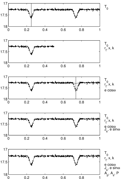
Figure 1: The five steps of obtaining the best initial guess for OGLE053312.82-700702.5. The values of the parameters in each step are given in Table 3. The line in the first panel is a smoothing of the data, performed by a running mean smoothing algorithm. The rest of the lines are EBAS models in the different steps of the algorithm. Note that the bottom panel presents the best initial guess and not the final solution. The vertical lines in the first and the third panels are EBAS best estimate for the centres of the two eclipses.

Table 3: The five steps of obtaining the initial guess for OGLE053312.82-700702.5.

Stage	$T_{0}\ \ \$	$r_{t}$	$x\ \ \$	$k$	$e\cos\omega$	$J_{s}$	$e\sin\omega$	$A_{p}$	$A_{s}\$	$P$	$\chi^{2}\$
1	729.87
2	729.85	0.2805	0.4911	0.6810
3	729.85	0.2805	0.4911	0.6810	-0.0184						2103.5
4	729.85	0.2805	0.4000	1.0000	-0.0184	1.0000	0.0000				323.9
5	729.85	0.2771	0.3806	0.9996	-0.0136	1.0213	-0.0003	0.9834	0.9998	5.394410	267.6
final	729.85	0.2697	0.3185	1.5087	-0.0134	1.0414	0.0143	0.3948	0.9927	5.394382	263.9

To estimate the uncertainties of the derived parameters, EBAS uses the Monte-Carlo bootstrap method, as described in Press et al. (1992). For each solution, we generated a set of 25 simulated lightcurves by using the values of the model at the original data points, with added normally distributed noise. The amplitude of the noise is chosen to equal the uncertainty of the data points. EBAS then proceeds to solve each of these lightcurves, using the simulated (”true”) values of $r_{t}$, $T_{0}$, $P$ and $e\cos\omega$ as initial guesses. EBAS sets the error of each parameter to be the standard deviation of its values in the sample of generated solutions. Section 5 analyses the performance of EBAS and finds that its error estimation is correct to a factor of about 2.

4 A new ’alarm’ statistic to assess the solution goodness-of-fit

During the development of EBAS we found that some solutions with low $\chi^{2}$ might be unsatisfactory. Fig 2 presents such a system solution, OGLE051331.74-691853.5, obtained manually by NZ04. While the value of $\chi^{2}$ is reasonable, the model deviates from the observations at the edges of the eclipses, as a visual inspection of the residuals, plotted as a function of phase, can reveal. This case shows that the $\chi^{2}$ statistic, while being the unchallenged goodness-of-fit indicator, can be low even for solutions which are not quite satisfactory. For such cases, human interaction is needed to improve the fit, or to otherwise decree the solution unsatisfactory. In order to allow an automated approach, an automatic algorithm must replace human evaluation.

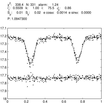
Figure 2: Lightcurve, solution and elements for OGLE051331.74-691853.5, as derived by NZ04. The solution is not optimal, as visual scrutiny of the edges of the eclipses may reveal.

We therefore defined a new estimator which is sensitive to the correlation between adjacent residuals of the measurements relative to the model. This feature is in contrast to the behaviour of the $\chi^{2}$ function, which measures the sum of the squares of the residuals, but is not sensitive to the signs of the different residuals and their order. For an estimator to be sensitive to the number of consecutive residuals with the same sign, one might use some kind of run test (e.g., Kanji, 1993). In such a test, the whole lightcurve is divided into separate sequential runs, where a ’run’ is defined as a maximal series of consecutive residuals (in the folded lightcurve) with the same sign. For example, if the residuals are $\{1,2,1,-3,-4,5,-2,-3\}$ (written in order of increasing phase) the four runs would be $\left\{\{1,2,1\},\{-3,-4\},\{5\},\{-2,-3\}\right\}$. Long runs might indicate that the residuals are not randomly distributed. For example, in Fig 2 a run of 13 negative residuals exists around phase $0.4$, and a run of 17 positive residuals exists around phase $0.65$.

Different approaches for residual diagnostics based on run tests may be found in the literature (e.g., Kanji, 1993). Lin’s cumulative residuals (Lin et al., 2002) is one example. We chose to define a new estimator which is sensitive both to the length of the runs and to the magnitude of the residuals, in units of their uncertainties.

Denoting by $k_{i}$ the number of residuals in the $i$-th run, we define the ’alarm’ $\mathcal{A}$ as:

$$\mathcal{A}=\frac{1}{\chi^{2}}\sum_{i=1}^{M}{\left(\frac{r_{i,1}}{\sigma_{i,1}}+\frac{r_{i,2}}{\sigma_{i,2}}+\cdots+\frac{r_{i,k_{i}}}{\sigma_{i,k_{i}}}\right)^{2}}-(1+\frac{4}{\pi})\ \ ,$$ (3)

where $r_{i,j}$ is the residual of the $j$-th measurement of the $i$-th run and $\sigma_{i,j}$ is its uncertainty. The sum is over all the measurements in a run and then over the $M$ runs. The $\chi^{2}$ is the known function:

$$\chi^{2}=\sum_{i=1}^{N}{\left(\frac{r_{i}}{\sigma_{i}}\right)^{2}}\ \ ,$$ (4)

where the sum is over all $N$ observations. Dividing by $\chi^{2}$ assures that, in contrast to $\chi^{2}$ itself, $\mathcal{A}$ is not sensitive to a systematic overestimation or underestimation of the uncertainties.

It is easy to see that $\mathcal{A}$ is minimal when the residuals alternate between positive and negative values, and that long runs with large residuals increase its value. The minimal value of the summation is exactly $\chi^{2}$, and therefore the minimal value of $\mathcal{A}$ is $-4/\pi$.

For $N$ uncorrelated Gaussian residuals, the expectation value for $\mathcal{A}$ can be calculated under the assumptions that $\chi^{2}=N$, and that $N$ is large enough to make the length of the runs be distributed geometrically for all practical purposes. According to this calculation, the expectation value of $\mathcal{A}$ as defined above vanishes.

To explore the behaviour of the new statistic we simulated residuals of normal random noise composed of 200, 500 and 1000 points, each of which for 100,000 times, and plotted in Fig 3 histograms of the $\mathcal{A}$ values. The solution of Fig 2 has indeed an ${\mathcal{A}}$ value of $1.24$, which is too high, as can be seen in Fig 3.

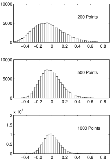
Figure 3: The distribution of $\mathcal{A}$ for normally distributed 200, 500 and 1000 random points.

When a solution shows high $\mathcal{A}$, EBAS performs additional simulated annealing searches with different initial guesses. In most cases, a few iterations that start in the parameter space not far away from the previously found minimum are sufficient to find a substantially better minimum. We stop this process when EBAS finds a new solution with low enough $\mathcal{A}$. If this approach does not lead to a solution with low enough $\mathcal{A}$, EBAS calls for visual inspection, and manually initialized optimization may be attempted. Our experience with the OGLE LMC data indicated that some systems simply cannot be modelled by the EBOP subroutines, either because the lightcurve is not of an eclipsing binary, or because EBOP is insufficiently accurate to model the light modulation.

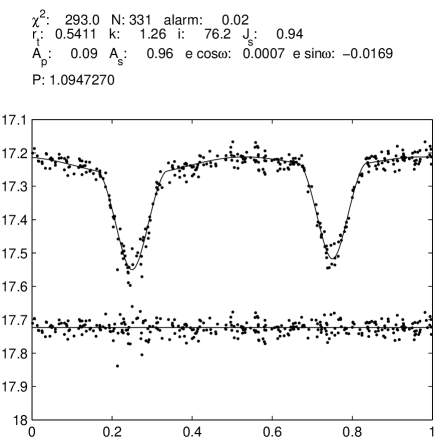
Figure 4: An improved solution relative to the one of Fig 2, with lower $\chi^{2}$ and $\mathcal{A}$.

Fig 4 shows the lightcurve of Fig 2 with its EBAS solution. Clearly, the code found a model with lower $\chi^{2}$ and better $\mathcal{A}$ value of $0.02$.

5 Testing the algorithm

To check the reliability of EBAS when applied to OGLE-like data, we performed a few tests. We analyzed a large sample of simulated lightcurves of eclipsing binaries, checked the obtained $\chi^{2}$ against the inserted noise, and examined the derived elements and their uncertainties versus the correct elements. The advantage of a simulated sample of lightcurves is the knowledge of the “true” elements, a feature that is missing, unfortunately, in real data. We also used simulations to estimate the sensitivity of the EBAS results to the assumption that there is no contribution of light from a third star, and to the assumption that the mass ratio is unity. We then compared the parameters derived by EBAS for real 509 OGLE LMC systems with the elements obtained manually by NZ04 with the EBOP code. The goal of this comparison was to find out how well EBAS performs as compared with manual finding of the elements with the same code. Finally, we compared our results with the recently derived elements of four eclipsing binaries in the LMC by González et al. (2005, hereafter GOMoM05), who analysed OGLE and MACHO photometry and a few radial-velocity measurements. The goal of this comparison was to compare the elements found by EBAS with elements found by using extra information on the same systems. This comparison is of particular interest because GOMoM05 used for their analysis not only lightcurves in three passbands, but also radial velocities, and they interpreted their data with the more sophisticated WD code.

5.1 Simulated lightcurves — comparison with the “true” elements

To check EBAS against simulated lightcurves we generated a sample of lightcurves with the EBOP subroutines and solved them with EBAS. To obtain an OGLE-like sample, the elements were taken from the NZ04 set of solutions for the OGLE LMC data, with $k$, the ratio of radii, chosen randomly from a uniform distribution between $0.5$ and $1$ (the NZ04 solutions had $k=1$, except for the relatively few systems with clearly total eclipses). For each simulated system we created a lightcurve with the original OGLE observational timings, and added random Gaussian noise, with an amplitude equal to the rms of the actual residuals relative to the NZ04 solution of that system. In total, 423 simulated lightcurves were created and solved.

To assess the goodness-of-fit of the solutions we calculated for each system the normalized $\chi^{2}$ of the EBAS solution, which is the sum of squares of the residuals, scaled by the uncertainty of each point, divided by the number of degrees of freedom of each solution. We compared this value with the “original $\chi^{2}$” of each lightcurve, which is the average of the sum of squares of the inserted errors around the original calculated lightcurve, again scaled by the uncertainty of each point. Fig 5 shows the $\chi^{2}$ of the solution versus the original one. The continuous line is the locus of points for which the two $\chi^{2}$s are equal. The figure shows that most points lie next to the line, which means that for each lightcurve the algorithm found a set of parameters that fit the data with residuals which are close, on the average, to the original scatter. While one can not be sure that global minima were found for all lightcurves, the fact that none of the solutions showed substantially large normalized $\chi^{2}$ is reassuring.

Figure 5: Simulation results: the derived vs. original normalized $\chi^{2}$.

Fig 6 shows the values of six of the derived elements of the simulated sample as a function of the original values. In order not to turn the plot too dense, we randomly choose only 100 systems for the display. The figure shows that the sum of radii, $r_{t}$, is reproduced quite well by the code, and so is $e\cos\omega$. For $x$, $e\sin\omega$ and $J_{s}$, EBAS produced slightly less accurate, but still quite good results. The parameter $k$ seems more difficult to determine, and its derived values coincide with the original ones only for lightcurves of high $S/N$ ratio. Still, the correlation between the original and derived $k$ values for the whole sample is 0.6, and we feel that allowing $k$ to vary is meaningful, except perhaps for very noisy lightcurves.

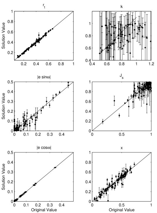
Figure 6: Simulation results: the derived vs. “true” elements.

It is well known that lightcurves of only one colour include degeneracy between few parameters. The values of those parameters deviate together from their true values, yielding almost as good solutions as the ones with the true values. To estimate the magnitude of this effect, we consider the deviations of the derived elements from their true values in our simulations and estimate the correlations between those deiviations. Fig 7 shows the correlation between the deviation of the $x$ parameter — $\Delta x$, and three other parameter deviations. The figure shows a small but somewhat significant correlation with $\Delta e\sin\omega$ and $\Delta k$, and high correlation with $\Delta r_{t}$. However, as the deviations of most of the $r_{t}$ values are quite small, we still suggest that the derived values of $r_{t}$ are valid. The figure also shows that there is no correlation between $\Delta J_{s}$ and $\Delta k$.

Figure 7: Correlation between the deviations from true values for four pairs of elements. The value of the corresponding correlation appears in each panel.

To explore the reliability of our uncertainty estimate we consider for each parameter $p$ the scaled error $\delta p=(p_{derived}-p_{original})/{\sigma_{p}}$, which measures the actual error, i.e. the difference between the derived and original values of $p$, divided by the uncertainty, $\sigma_{p}$, as estimated by EBAS. We plotted in Fig 8 histograms of scaled errors for eight parameters. With correct uncertainties, the distributions of the scaled errors should all have Gaussian shape and variance of unity. Wide distribution indicates that our estimate for the error might be too small. We can see that all distributions — except that of $\delta k$, the most problematic parameter — are close to have a Gaussian shape and width of unity, even though asymmetry and outliers increase the rms value by up to a factor of two.

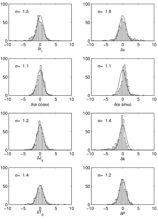
Figure 8: Simulation results: the distribution of the scaled errors for eight EBAS parameters. For comparison, Gaussian distributions with unity variance are plotted. The rms of each distribution is given in each panel.

5.2 The sensitivity of the elements to two simplifying assumptions

The present embodiment of EBAS assumes that $L_{3}$ is zero and the mass ratio is unity. The former assumption implies that all the light of the system is coming from the two components of the binary. This is not necessarily the case, as a third star, either a background star or a distant companion of the system, could also contribute to the total light of the system. Failure to realize the contribution of a third star could result in underestimation of the depth of the eclipses, which induces further systematic errors in the derivation of the binary elements. To estimate the error induced by the value assigned to the light of a third star, we generated lightcurves identical to the ones of the previous simulation, except that we set $L_{3}=0.1$ for all of them. We then solved them using EBAS as before, assuming $L_{3}=0$. The comparison between the solutions and the original values for three elements — the sum of radii, the impact parameter and the ratio of radii, is plotted in Fig 9.

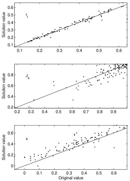
Figure 9: Simulation results: the effect of the assumption $L_{3}=0$. The derived values of the parameters, assuming $L_{3}=0$ vs. the true values for systems with $L_{3}=0.1$.

The sum of radii, which is mainly sensitive to the eclipse shape, is almost not affected by the different value of $L_{3}$. On the other hand, the values of the surface brightness ratio show a relatively large spread relative to the “true” values. However, this spread is not larger than the corresponding one in Fig 6. This means that the assumption $L_{3}=0$ did not increase substantially the error of the derived values of the surface brightness ratios. The impact parameter values show the clearest effect. The derived values are systematically larger than the true values, in order to account for the shallower eclipses interpreted by EBAS, because of the $L_{3}=0$ assumption.

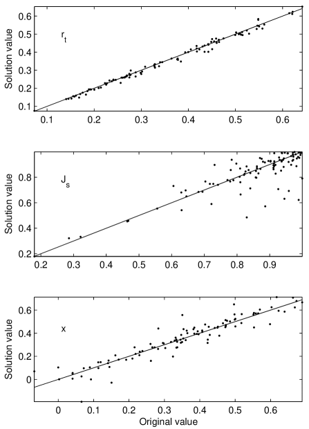
Figure 10: Simulation results: the effect of the assumption that the mass ratio is unity. The derived values of the parameters, assuming $q=1.0$ vs. the true values for systems with $q=0.8$.

We performed similar simulation to estimate the effect of the assumption that $q=1$. The results are plotted in Fig 10. The simulations show that the assumption of $q=1$ does not affect substantially the derived values of the sums of radii, the surface brightness ratios and the impact parameters.

5.3 The real OGLE LMC lightcurves — comparison with manual solutions

As another test of EBAS, we applied our algorithm to the OGLE LMC lightcurves solved by NZ04 using manual iterations with EBOP. Note that we compare here the “manual” fits by NZ04 with those of EBAS for the real systems, while Fig 5 compares the original scatter of simulated lightcurves with that resulting from the fit.

After discarding 58 solutions with high alarm or high $\chi^{2}$, we were left with 451 binaries. To compare EBAS solutions with those of NZ04, we derive for each EBAS solution a normalized $\chi^{2}$, which is equal to the unnormalized one, given by Eqn. 4, divided by the number of observed points minus the number of fitted parameters. Fig 11 plots a histogram of the NZ04 normalized $\chi^{2}$’s minus those of EBAS.

The comparison shows that the two sets of solutions are comparable. In fact, NZ04 achieved better solutions for 156 systems, out of which only 2 systems, which can be seen in the figure, had smaller normalized $\chi^{2}$ by more than 3%. On the other hand, EBAS solved 295 systems with lower $\chi^{2}$, out of which 156 solutions had smaller normalized $\chi^{2}$ by more than 3%. We therefore suggest that EBAS found slightly better solutions for most of the binaries analysed by NZ04.

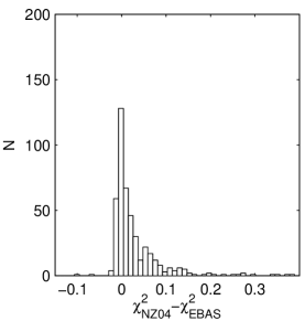
Figure 11: Histogram of difference between NZ04 solutions $\chi^{2}$ and EBAS solutions $\chi^{2}$.

5.4 Four eclipsing binaries analysed by GOMoM05 — comparison with the WD solutions

Very recently, GOMoM05 derived absolute parameters for eight eclipsing binaries in the LMC, using photometric data from MACHO (Alcock et al., 1997) together with a few radial-velocity measurements. OGLE data is available for four of these systems, and GOMoM05 used these data as well. To compare the values of GOMom05 with EBAS, we solved for these four systems and plotted their solutions in Fig 12.

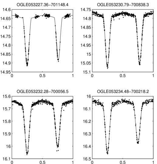
Figure 12: The EBAS solutions for the OGLE lightcurves of the four binaries analysed by GOMoM05.

Before comparing the results of the two solutions, a word of caution is needed. GOMoM05 used the WD code, derived the temperature ratio from the spectroscopic data, and used lightcurves of three different colours for each of the four systems. Our solution is based on the OGLE $I$-band data only. We therefore choose to compare only the geometric parameters of the systems, namely the sum of radii, the inclination, the ratio of radii and the eccentricity. Table 4 brings the detailed comparison. For each of the four systems, the first line in the table gives the GOMoM05 elements, while the second line gives EBAS’s. It is reassuring that despite all the differences in the derivation of the two sets of elements, all values of all geometric elements agree within $1$–$2$ $\sigma$ of each other. Indeed, the large differences in the values of the ratio of radii of OGLE051804.81-694818.9 and OGLE052235.46-693143.4 are only caused by a switch between the primary and the secondary in the GOMoM05 solution. The reciprocal GOMoM05’s values are within 1$\sigma$ of the EBAS results.

Table 4: Elements of four binaries: comparison between GOMoM05 (first row) and EBAS (second row) solutions.

System	$r_{t}$	$i$	$k$	$e$
OGLE052232.68-701437.1	$0.426\pm 0.018$	$78.0\pm 0.8$	$0.84\pm 0.10$	$0.025\pm 0.006$
	$0.458\pm 0.007$	$77.0\pm 0.4$	$0.99\pm 0.07$	$0.044\pm 0.014$
OGLE050828.13-684825.1	$0.458\pm 0.009$	$77.9\pm 0.8$	$0.80\pm 0.20$	$0.043\pm 0.006$
	$0.475\pm 0.003$	$77.3\pm 0.2$	$0.84\pm 0.12$	$0.043\pm 0.001$
OGLE051804.81-694818.9	$0.498\pm 0.010$	$81.3\pm 0.8$	$0.75\pm 0.08$	0
	$0.496\pm 0.004$	$81.0\pm 0.3$	$1.49\pm 0.04$	$0.003\pm 0.004$
OGLE052235.46-693143.4	$0.485\pm 0.017$	$80.1\pm 1.4$	$0.73\pm 0.09$	0
	$0.490\pm 0.007$	$80.4\pm 0.8$	$1.49\pm 0.25$	$0.015\pm 0.010$

6 Discussion

We have shown that it is possible to solve lightcurves of eclipsing binaries with a fully automated algorithm which is based on the EBOP code. Our simulations have shown that the results of EBAS are close to the “real” ones and that EBAS results for most cases have a quality which is better than is achieved with human interaction.

Although the EBOP code does not include the sophistications offered by, e.g., the widely used Wilson-Devinney programme, it has the advantage of being simple and of producing parameters closely related to the real information content of the lightcurve (e.g., surface brightness instead of effective temperature). In addition, it does take into account not only reflection effects, but also tidal deformation of components (even though in a primitive way), so that it remains useful for systems with moderate proximity effects. Comparison with the recent work of GOMoM05 who used the WD code to analyse three colour photometry, radial-velocity and spectroscopic data of four systems shows that the present version of EBAS recovers quite well the sum of radii, the inclination and the ratio of radii.

It is interesting to compare the speed of the present version of EBAS with the very fast automated DEBiL algorithm (Devor, 2005), which was used to derive the elements of almost 10,000 eclipsing binaries in the Galactic bulge. On the average, it took EBAS 50 seconds CPU time to solve one orbit on an AMD Opteron, 250 2.46GHz, 64-bit machine, while error estimation took another 100 seconds. This is about 3 times longer than it took Devor to solve an orbit with his DEBiL with a SUN UltraSPARC5 333MHz. Applying EBAS to 10,000 systems is therefore feasible.

EBAS uses two redundant techniques to ensure the finding of the global minimum — a search for the minimum with simulated annealing and consultation with the new alarm $\mathcal{A}$. The simulated annealing technique causes heavy computation load on EBAS, and if the number of lightcurves is too large, the demanding parameters of the annealing can be slightly relaxed, since we can rely on the alarm to warn us if the global minimum is not reached.

In the next papers we plan to apply EBAS to the sample of the LMC (Mazeh, Tamuz & North 2005, Paper II) and SMC OGLE data. Obviously, when EBAS is applied to real data, one should carefully examine the implication of the specific choices done for the nonvariable parameters, the values of the mass ratio, the fractional light of a possible third star and the values for the limb and gravity darkening. However, the goal of applying EBAS to such large datasets is not to derive the exact parameters of a particular system. Instead, the aim is to study statistical features of the short-period binaries, like their frequency and period distribution. In that sense, the set of data points we use includes the photometry obtained for all the eclipsing binaries found in the sample. For the OGLE LMC data, this is about 300 points for more than 2000 systems, which adds up to about 0.6 millions points, admittedly with low $S/N$ ratio. Such a huge dataset should allow us to study some statistical features of the short-period binaries.

An obvious extension of EBAS would be to allow for automated derivation of the mass ratio, the light of a third star, and even the limb and gravity darkening. This can not be done with OGLE data of the LMC, but would be possible for systems with better data and more than one colour photometry. For close binaries with strong proximity effects we plan to allow EBAS to use the WD code. In principle, the approach should be the same, with the same procedure to find the best initial guess, the same simulated annealing search and the same error estimation. The development of these capacities of EBAS are deferred to a later paper.

Finally, we plan to construct an automated algorithm to derive the masses of the two stars in each eclipsing binary in the LMC, in a similar approach to the one presented by J. Devor in the “Close Binaries in the 21st Century: New Opportunities and Challenges” meeting. Our approach relies on the fact that we know the distance to all the binaries in our neighbouring galaxy, up to a few percent, and therefore know the absolute magnitude of the LMC OGLE systems. OGLE data includes some measurements in the $V$ band for each star in the LMC, and therefore the available absolute magnitude information includes two colours. Furthermore, MACHO data (Alcock et al., 1997) is also available for most of these systems. This should suffice to derive a crude estimate of the masses and ages of all the eclipsing binaries in the OGLE LMC dataset.

References

- Alcock et al. (1997) Alcock C., Allsman R. A., Alves D., Axelrod T. S., Becker A. C., 1997, AJ, 114, 326
- Devor (2005) Devor J., 2005, ApJ accepted (astro-ph/0504399)
- Eggleton (1983) Eggleton P. P., 1983, ApJ, 268, 368
- Etzel (1980) Etzel P. B., 1980, EBOP User’s Guide. Dep. of Astronomy, Univ. of California, third edn
- González et al. (2005) González J. F., Ostrov P., Morrell N., Minniti D., 2005, ApJ, 624, 946
- Kanji (1993) Kanji G. F., 1993, 100 Statistical Tests. Sage Publications, London
- Lin et al. (2002) Lin E. Y., Wei L. J., Ying Z., 2002, Biometrics, 58, 1
- Marquardt (1963) Marquardt D. W., 1963, Journal of the Society for Industrial and Applied Mathematics, 11, 431
- North & Zahn (2003) North P., Zahn J.-P., 2003, A&A, 405, 677
- North & Zahn (2004) North P., Zahn J.-P., 2004, New Astronomy Review, 48, 741
- Popper & Etzel (1981) Popper D. M., Etzel P. B., 1981, AJ, 86, 102
- Press et al. (1992) Press W. H., Teukolsky S. A., Vetterling W. T., Flannery B. P., 1992, Numerical recipes in FORTRAN. The art of scientific computing. Cambridge: University Press, —c1992, 2nd ed.
- Ribas et al. (2000) Ribas I., Guinan E. F., Fitzpatrick E. L., DeWarf L. E., Maloney F. P., Maurone P. A., Bradstreet D. H., Giménez Á., Pritchard J. D., 2000, ApJ, 528, 692
- Udalski et al. (1998) Udalski A., Soszynski I., Szymanski M., Kubiak M., Pietrzynski G., Wozniak P., Zebrun K., 1998, Acta Astronomica, 48, 563
- Udalski et al. (2000) Udalski A., Szymanski M., Kubiak M., Pietrzynski G., Soszynski I., Wozniak P., Zebrun K., 2000, Acta Astronomica, 50, 307
- Wyithe & Wilson (2001) Wyithe J. S. B., Wilson R. E., 2001, ApJ, 559, 260
- Wyrzykowski et al. (2003) Wyrzykowski L., Udalski A., Kubiak M., Szymanski M., Zebrun K., Soszynski I., Wozniak P. R., Pietrzynski G., Szewczyk O., 2003, Acta Astronomica, 53, 1