Absolute measurement of the unresolved cosmic X-ray background
in the 0.5–8 keV band with CHANDRA

Abstract

We present the absolute measurement of the unresolved 0.5–8 keV cosmic X-ray background (CXB) in the Chandra Deep Fields (CDFs) North and South, the longest observations with Chandra (2 Ms and 1 Ms, respectively). We measure the unresolved CXB intensity by extracting spectra of the sky, removing all point and extended sources detected in the CDF. To model and subtract the instrumental background, we use observations obtained with ACIS in stowed position, not exposed to the sky. The unresolved signal in the 0.5–1 keV band is dominated by diffuse Galactic and local thermal-like emission. We find unresolved intensites in the 0.5–1 keV band of $(4.1\pm 0.3)\times 10^{-12}$ ergs cm^-2 s^-1 deg^-2 for CDF-N and $(5.0\pm 0.4)\times 10^{-12}$ for CDF-S. In the 1–8 keV band, the unresolved spectrum is adequately described by a power law with a photon index $\Gamma=1.5^{+0.5}_{-0.4}$ and normalization $2.6\pm 0.3$ photons cm^-2 s^-1 keV^-1 sr^-1 at 1 keV. We find unresolved CXB intensities of $(1.04\pm 0.14)\times 10^{-12}$ ergs cm^-2 s^-1 deg^-2 for the 1–2 keV band and $(3.4\pm 1.7)\times 10^{-12}$ ergs cm^-2 s^-1 deg^-2 for the 2–8 keV band. Our detected unresolved intensities in these bands significantly exceed the expected flux from sources below the CDF detection limits, if one extrapolates the $\log{N}/\log{S}$ curve to zero flux. Thus these background intensities imply either a genuine diffuse component, or a steepening of the $\log{N}/\log{S}$ curve at low fluxes, most significantly for energies $<$2 keV. Adding the unresolved intensity to the total contribution from sources detected in these fields and wider-field surveys, we obtain a total intensity of the extragalactic CXB of $(4.6\pm 0.3)\times 10^{-12}$ ergs cm^-2 s^-1 deg^-2 for 1–2 keV and $(1.7\pm 0.2)\times 10^{-11}$ ergs cm^-2 s^-1 deg^-2 for 2–8 keV. These totals correspond to a CXB power law normalization (for $\Gamma=1.4$) of 10.9 photons cm^-2 s^-1 keV^-1 sr^-1 at 1 keV. This corresponds to resolved fracations of $77\pm 3$% and $80\pm 8$% for 1–2 and 2–8 keV, respectively.

1. Introduction

Measurement of the cosmic X-ray background (CXB) has been a major effort in X-ray astronomy since it was first discovered in rocket flights in the 1960’s (Giacconi et al., 1962). The total spectrum of the CXB has been studied at energies up to 50 keV by HEAO–1 and rocket experiments (e.g., Marshall et al., 1980; McCammon et al., 1983; Garmire et al., 1992; Revnivtsev et al., 2005); for a review of pre-ROSAT results, see McCammon & Sanders (1990). It was later studied in different parts of the 0.5–10 keV interval by ROSAT (e.g., Snowden et al., 1995; Georgantopoulos et al., 1996; Kuntz et al., 2001), ASCA (e.g., Gendreau et al., 1995; Chen et al., 1997; Miyaji et al., 1998; Ueda et al., 1999; Kushino et al., 2002), BeppoSAX (e.g., Parmar et al., 1999; Vecchi et al., 1999), XMM-Newton (Lumb et al., 2002; De Luca & Molendi, 2004, hereafter DM04) and RXTE (Revnivtsev et al., 2003). Deep observations with Chandra were used to study the component of the 0.5–8 keV CXB that resolves into point sources (e.g., Brandt et al., 2001b; Giacconi et al., 2002, and later works). Markevitch et al. (2003) used Chandra ACIS-S to study the diffuse components at 0.5–2 keV. For $E<1$ keV, the CXB is due to extragalactic and local discrete sources, as well as diffuse (Galactic and possibly Solar System) components (e.g., Kuntz & Snowden, 2000; Cravens, 2000). Above 1 keV, the CXB is primarily extragalactic in origin, and is well fit by a power law with a photon index of 1.4.

As X-ray telescopes have improved in angular resolution, more and more of the CXB above 1 keV has been resolved into point sources, mostly active galactic nuclei (see Brandt & Hasinger, 2005, for a review). However there still remains unresolved CXB flux of unknown origin and uncertain intensity. Moretti et al. (2003, hereafter M03) added the contributions of detected point sources from a variety of narrow and wide-field X-ray surveys, and found resolved fractions of the extragalactic CXB of $94\pm 7$% for the 0.5–2 keV band and $89^{+8}_{-7}$% for the 2–10 keV band. Worsley et al. (2005) performed a similar study to find the fraction of the CXB that is resolved as a function of energy, using the detected sources from Chandra and XMM-Newton observations, and total CXB estimates from the XMM-Newton study of DM04. They found that the resolved fraction of the extragalactic background decreases significantly at higher energies, from $\sim$80% at $\sim$1 keV to $\sim$60% at 7 keV. This leaves room for a possible population of faint sources that have yet to be detected, as well as truly diffuse components, including exotic ones such as emission from dark matter particle decay (e.g., Abazajian et al., 2001). There remains a great deal of uncertainty in the resolved fraction, largely due to uncertainty in the absolute flux of the CXB, and to cross-calibration uncertainties between different measurements.

Due to its angular resolution, Chandra is by far the best instrument for detecting point sources to very low fluxes and resolving the CXB. This study uses Chandra ACIS-I for an absolute measurement of the intensity of the unresolved X-ray background in the energy range 0.5–8 keV, after the exclusion of sources down to the lowest fluxes detectable in the deepest current exposures. We use data from the Chandra Deep Fields (CDFs, e.g., Brandt et al., 2001b; Giacconi et al., 2002), which were designed specifically to resolve as much of the extragalactic CXB as possible. As a byproduct of our measurement, we add our unresolved flux to the contributions from known sources (from the CDFs and other observations) to obtain the total intensity of the CXB. This measurement has not previously been performed with Chandra because of difficulties in determining the instrumental ACIS backgrounds. Recent calibration using the ACIS detectors stowed out of the focal plane have made this study possible. Throughout this paper we will define the power law photon index as $\Gamma$, where the photon flux $F\propto E^{-{\Gamma}}$, and we will use 68% errors.

2. Data and strategy

We use two of the deepest observations of the X-ray sky ever performed, the Chandra Deep Fields North and South (CDF-N and CDF-S), which have total exposure times of $\sim$2 Ms and 1 Ms, respectively. These fields are located in regions of low $N_{\rm H}$, away from any bright features in the Galactic emission. Each CDF data set is made up of a number of observations from different epochs covering approximately the same field. We use all observations taken after 2000 January 21 when the ACIS focal plane temperature was set at $-120$ ^∘C; this is the period for which the detector backgound calibration is applicable. The observations are listed in Table 1.

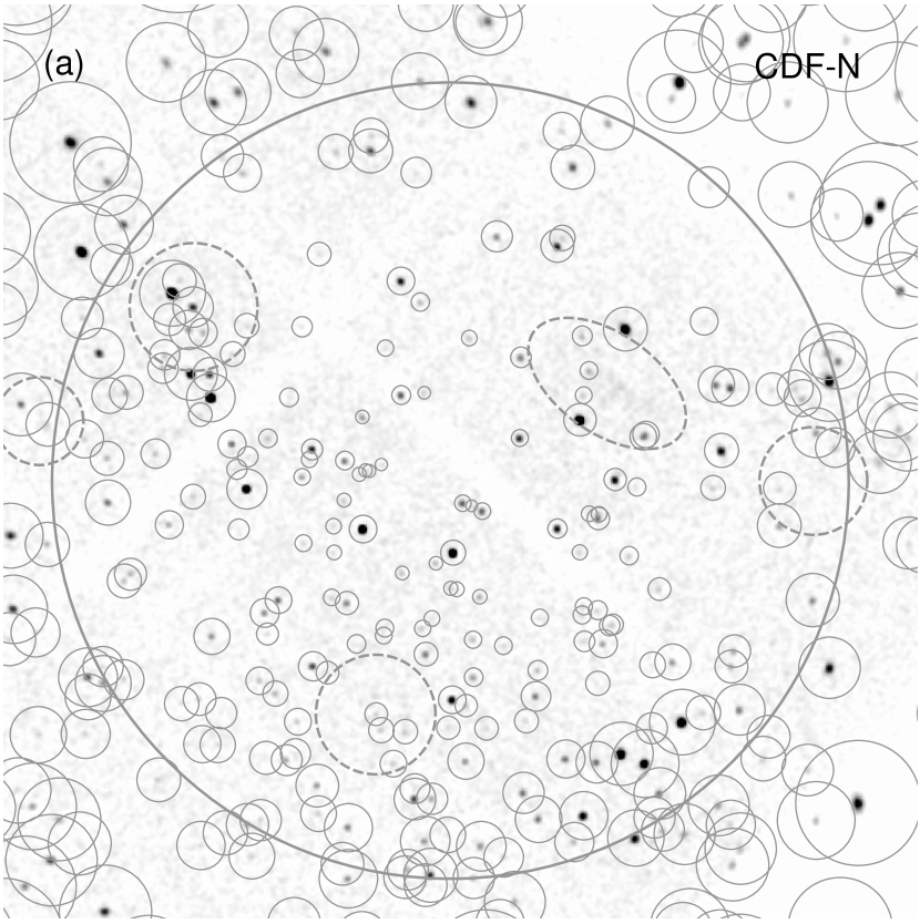
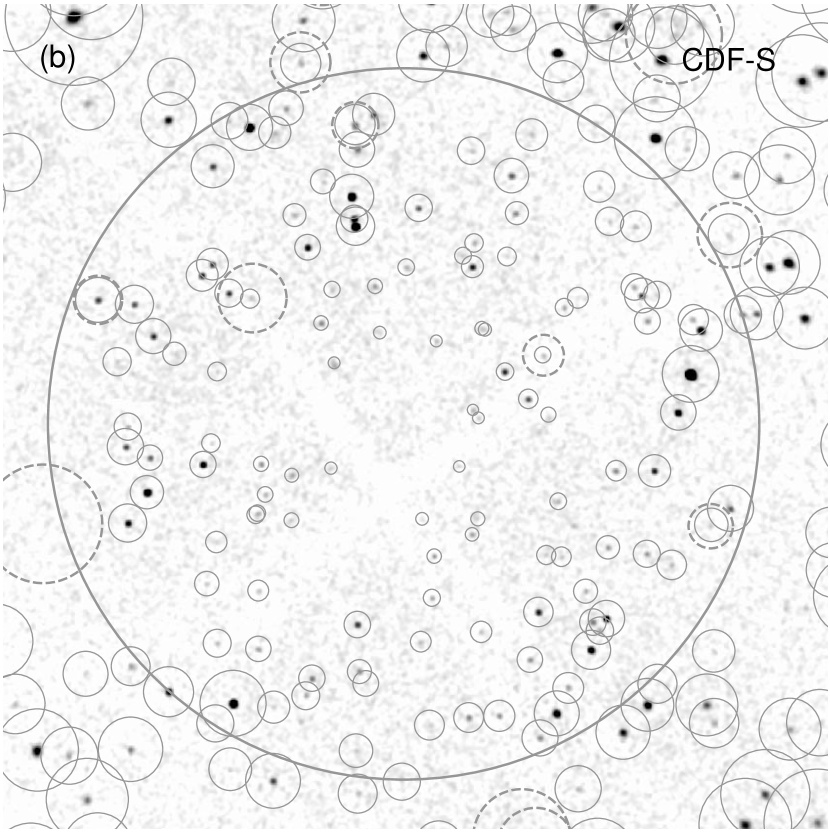
Figure 1.— Full (1.9 Ms and 0.8 Ms) 0.5–8 keV images for (a) CDF-N and (b) CDF-S. Point source exclusion regions, with source positions and fluxes taken from A03 are shown (for illustration, we use regions for the particular aimpoints of ObsIDs 3294 and 582). Diffuse source exclusion regions are shown as dashed lines. The central 5′ radii around the aimpoints (the regions used in our analysis) are shown as thick lines.

Table 1Chandra Deep Field exposures used for spectral analysis

ObsID	Obs. start date	ACIS mode	Total exp. (ks)	Clean exp. (ks)	RA	Dec
CDF-N
1671	2000-11-21	F	168.1	97.4	12 37 04.30	+62 13 04.2
2344	2000-11-24	F	93.3	0.0	12 37 04.17	+62 13 03.5
2232	2001-02-19	F	131.8	102.7	12 36 35.96	+62 14 37.4
2233	2001-02-22	F	64.7	37.3	12 36 35.66	+62 14 35.5
2423	2001-02-23	F	69.8	59.1	12 36 35.66	+62 14 35.7
2234	2001-03-02	F	167.2	127.6	12 36 34.70	+62 14 28.8
2421	2001-03-04	F	63.2	47.7	12 36 34.39	+62 14 26.2
Total CDF-N F	$\cdots$	F	758.0	471.7	$\cdots$	$\cdots$
3293	2001-11-13	VF	161.4	113.0	12 36 51.77	+62 13 03.2
3388	2001-11-16	VF	49.6	0.0	12 36 51.80	+62 13 03.5
3408	2001-11-17	VF	67.7	37.3	12 36 51.78	+62 13 03.1
3389	2001-11-21	VF	125.6	0.0	12 36 51.70	+62 13 04.5
3409	2002-02-12	VF	82.5	62.2	12 36 36.93	+62 14 41.1
3294	2002-02-14	VF	170.8	107.8	12 36 36.92	+62 14 41.1
3390	2002-02-16	VF	164.7	94.4	12 36 36.92	+62 14 41.0
3391	2002-02-22	VF	164.7	122.4	12 36 36.93	+62 14 41.1
Total CDF-N VF	$\cdots$	VF	986.9	537.1	$\cdots$	$\cdots$
CDF-S
441	2000-05-27	F	57.1	20.7	03 32 26.84	-27 48 17.9
582	2000-06-03	F	132.2	94.3	03 32 26.91	-27 48 16.6
2406	2000-12-10	F	30.7	20.7	03 32 28.41	-27 48 38.3
2405	2000-12-11	F	60.5	30.1	03 32 28.88	-27 48 45.3
2312	2000-12-13	F	125.3	84.0	03 32 28.34	-27 48 38.8
1672	2000-12-16	F	96.3	74.7	03 32 28.78	-27 48 46.3
2409	2000-12-19	F	70.2	55.0	03 32 28.09	-27 48 40.4
2313	2000-12-21	F	131.8	97.5	03 32 28.10	-27 48 40.4
2239	2000-12-23	F	132.2	91.2	03 32 28.10	-27 48 40.3
Total CDF-S	$\cdots$	F	836.5	568.0	$\cdots$	$\cdots$

To exclude point sources down to as low fluxes as possible, we will in effect use the full (2 or 1 Ms) exposures (including several observations prior to 2000 January 21), by utilizing the source lists from Alexander et al. (2003, hereafter A03), who performed detailed source detection for these fields. For CDF-S, the A03 catalog has the same flux limits and is almost identical to the catalog of Giacconi et al. (2002), although with more accurate source positions. For each observation we only use the central 5′ radius around the aimpoint, where the source detection flux limits are lowest and the Chandra point-spread function (PSF) has a radius $\simeq$1″–3$\farcs$5, narrow enough to effectively separate source and background photons.

The main difficulty in such studies with ACIS (and with XMM-Newton, for that matter) is subtracting the detector background, which consists of quiescent and flare components. As we will see in this paper, the quiescent background is $\sim$5 and $\sim$25 times larger than the unresolved sky signal for the 1–2 keV and 2–8 keV bands, respectively, and so requires very careful subtraction. We model the quiescent background using the ACIS stowed background calibration, which was performed from 2002 to 2005.

The CDF data were taken with ACIS-I, which is better suited than ACIS-S for absolute CXB measurements, due to a lower and much more stable detector background. At our present level of understanding, difficulty in removing the detector background flares makes this study impossible with ACIS-S (Markevitch et al., 2003), but it is possible to clean flares out to very high precision for ACIS-I. To remove low-level flares, we use time filtering with much stricter criteria than those normally used for extended source analysis, discarding 39% of the total CDF exposure (see § 4.2). Since the ACIS stowed dataset is currently only 236 ks long, this does not limit our accuracy which is dominated by the statistical and systematic uncertainties of the stowed dataset.

For our measurements we divide the CDF data into three subsets: the more recent CDF-N observations taken in Very Faint (VF) ACIS mode (see § 3.3), the earlier Faint (F) mode CDF-N observations, and the CDF-S data, also in F mode, hereafter CDF-N VF, CDF-N F, and CDF-S. The most reliable measurement in the 2–8 keV band comes from the CDF-N VF subset, which were taken within a year of the earliest stowed observations, after which we can say with reasonable confidence that the quiescent background did not change (§ 4.1.2). We will find, however, that the two earlier datasets give results in good agreement with CDF-N VF, so we will average all three.

3. Data preparation

For each observation, our processing of the X-ray event lists is almost identical to the standard CIAO pipeline Level 2 processing. The only minor difference is that in removing bad columns, we do not also exclude adjacent columns as in the standard pipeline.

3.1. Coordinate registration

For the purpose of this work we require the individual exposures of each of the CDF fields to be aligned as accurately as possible. We register the reference frame of each exposure by first detecting point sources using a wavelet detection algorithm (Vikhlinin et al., 1998). We then translate the images to align the brightest 20–50 detected sources over the entire field of view, with 0.5–8 keV fluxes between $5\times 10^{-4}$ and 0.02 counts s^-1, to the corresponding RA, Dec positions in the A03 catalog. The A03 positions were themselves registered using comparison to accurate radio positions. We verify the accuracy of our registration by eye for each observation. Simple translation of the images, by not more than 2$\farcs$6 for any observation, is sufficient to register the positions to better than $0\farcs 5$.

3.2. Source exclusion

For each of the exposures in Table 1, we extract spectra of the sky excluding point and diffuse sources. We use the catalog of A03, after running our own source detection (described later in § 7.1) and obtaining essentially identical source catalogs. The A03 flux limits at the aimpoint for CDF-N are $2.5\times 10^{-17}$ ergs cm^-2 s^-1 and $1.4\times 10^{-16}$ ergs cm^-2 s^-1 for 0.5–2 and 2–8 keV, and for CDF-S are a factor of 2 higher. We include only the central 5′ around the aimpoint, because at greater off-axis angles the Chandra PSF becomes too large for our purposes. Around each point source we define a circular exclusion region. An estimate for the 90% encircled energy radius (at $E=1.5$ keV) as a function of the off-axis angle $\theta$ is given approximately by:

$$r_{90}\simeq 1\arcsec+10\arcsec(\theta/10\arcmin)^{2}.$$ (1)

To be sure to fully exclude source photons from the wings of the PSF, we multiply $r_{90}$ by a factor that varies depending on the flux of the excluded source. We find that it is sufficient to use exclusion radii of 4.5, 6, and 9 times $r_{90}$ for sources with $<100$, $100-1000$, and $>1000$ total source photons, respectively, in the 0.5–8 keV energy band. Because the aimpoints of the observations differ by up to 4′, we define the exclusion regions separately for each observation. Using a model for the ${\it Chandra}$ PSF (from the Chandra CALDB), we find that after such source exclusion, the “missed” source flux due to PSF scattering is $<$0.1% of the total source flux. This will correspond to only $\lessapprox$5% of the unresolved background intensity (§ 6.1).

We also exclude detectable extended sources. For CDF-N we use the diffuse source regions given in Table 1 of Bauer et al. (2002), multiplying the dimensions by a factor of 1.5 to ensure that diffuse source photons on the edges are excluded. For CDF-S we use the sources in Table 5 of Giacconi et al. (2002), and multiply the FWHM values by 5 to obtain the exclusion radii. The surface brightness of these extended sources is 2–3 times lower than the unresolved CXB brightness that we will obtain, so the details of source exclusion regions should not be important; we verify this assumption in § 7.1. In Fig. 1 we show images with exposures of 1.9 Ms and 0.8 Ms (after cleaning) of the CDF-N and CDF-S fields for 0.5–8 keV, with the point source and extended source exclusion regions.

3.3. VF mode background filtering

Seven of the CDF-N exposures (Table 1) were taken in VF ACIS telemetry mode, for which the detector background can be reduced significantly by rejecting events with signal above the split threshold in any of the outer pixels of the 5 x 5 pixel event island, after an approximate correction for the charge transfer inefficiency (CTI, Vikhlinin, 2002). This makes the instrumental background lower (by $\sim$20% for the 2.3–7.3 keV band for the front-illuminated (FI) chips such as ACIS-I) more spatially uniform, and more stable (see § 4.1.2). This filtering makes the CDF-N VF observations the most reliable for measurements for $E>2$ keV. The stowed dataset was taken in VF mode, so the same additional filtering is applied when appropriate.

The CDF-N VF data were taken with an onboard upper telemetry cutoff of 3025 PHA channels. This means that any events with a PHA_RO (the value of PHA before gain correction) $>$ 3025 ADU, corresponding to $\sim$12 keV, will not appear in the event lists. Therefore some events with energies $<$ 12 keV after gain correction, but with PHA_RO $>$ 3025, will be missing from the observed 9–12 keV count rate. Because we use the 9–12 keV count rate to normalize the stowed background, which does not have such a cutoff (§ 4.1.3), this effect may impact our results.

We tested for the effects of the PHA cutoff by examining telemetered data that does not have such a cutoff, including some sky observations as well as the stowed exposures. In all cases, a cut of PHA_RO $<$ 3025 produces a 1% difference in the 9–12 keV count rate for the full ACIS-I field of view. However, the missing events are found near the edges of the I-array, because the CTI correction, which moves energy upwards, is less strong there. The difference is negligible in the central 5′ region for which we extract spectra and normalize the background. Therefore, the upper telemetry cutoff has a no significant effect on our results.

4. Instrumental background

The total observed background spectrum for ACIS-I consists of four separate components: (1) the real cosmic background signal, (2) quiescent and (3) flaring detector backgrounds due mainly to particles of different energies, and (4) a readout artifact from the sources in the field of view due the finite readout time of the ACIS detectors, which for our purposes can be treated as a background. Accurate removal of the detector backgrounds is the key aspect of this analysis, so we discuss this in detail.

4.1. Quiescent background

The quiescent instrumental background of the ACIS detectors is due to interactions of the CCDs and surrounding materials with high-energy particles, and has been measured first by studying data taken in Event Histogram mode (that does not telemeter imaging information) with ACIS stowed inside the detector housing (Biller et al., 2002), later by briefly observing the dark Moon, and finally by taking long exposures in full imaging mode with ACIS stowed. For the latter measurement, the ACIS position inside the housing was selected to minimize the flux from the internal calibration source spectral lines. The satellite was in a regular region of the orbit where science observations are performed (i.e., not in the radiation belts) during these observations. The detector housing blocks celestial X-rays and low-energy particles that cause flares (§ 4.2) but does not affect the quiescent background rate by any detectable amount, as we shall see from comparison with the dark Moon data (§ 4.1.1).

Thus the ACIS-stowed dataset, which we use here, accurately represents the quiescent background in ACIS sky exposures. As of fall 2005, a total of 236 ks of stowed background data are available, accumulated during 2002–2005. Due to telemetry limitations, the stowed data were taken only with chips I0, I2, I3, S1, S2, and S3; the stowed background for the I1 chip is a slightly scaled and reprocessed copy of the I0 data. As we discuss in § 7.2, this has no significant effect on the results.

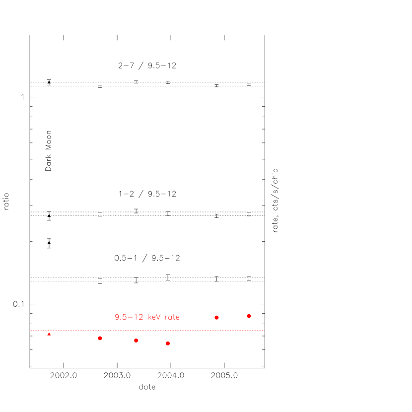
Figure 2.— Ratios of count rates in various bands to the 9.5–12 keV count rate (shown at bottom) for ACIS-I dark Moon (triangles) and stowed observations. Pairs of lines are $\pm$2%. A deviation in the 0.5–1 keV Moon data is an astrophysical signal (Wargelin et al., 2004).

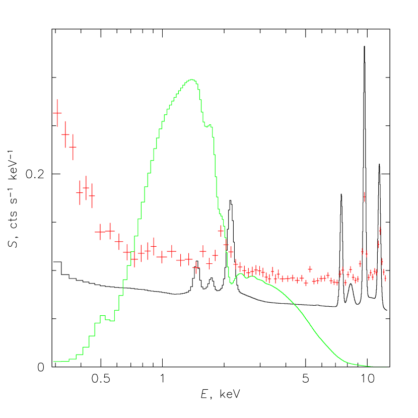
Figure 3.— Spectral shape of the ACIS-I quiescent background (solid dark line), along with a typical power-law sky spectrum (solid gray) and the average spectrum of the most common ACIS-I flare species (crosses). The flares and quiescent background are normalized to have the same 9–12 keV count rate.

The overall intensity of the quiescent background varies at the 10–20% level (showing a correlation with the solar cycle), but its spectral shape is remarkably stable. Fig. 2 shows the ratios of rates in three interesting bands to that in the 9.5–12 keV band (dominated by the fluorescent gold lines, see Fig. 3), for separate $\sim$50 ks exposures included in the ACIS-stowed dataset, and for the 14 ks dark Moon dataset.

4.1.1 Absence of any blocked component in the stowed background

The first important thing to note from Fig. 2 is that the dark Moon spectrum is the same as the stowed background for $E>1$ keV; the 2–7/9.5–12 keV rate ratios are consistent for the two datasets. For chips I2 and I3, the ratio for the dark Moon is $1.01\pm 0.03$ times that for the corresponding stowed data (note that in Fig. 2, chips I2 and I3 for the Moon are compared to chips I0, I2, and I3 for the stowed data, hence a small difference). From a separate Moon observation taken 2 months earlier, the ratio for chip S2, also an FI chip, is $0.99\pm 0.04$ times that for the S2 stowed data (not used in this analysis). The average of these factors is $1.00\pm 0.02$, which indicates that any possible quiescent sky background component not present in the stowed background is essentially zero for FI chips. For S3, a back-illuminated (BI) chip which is more strongly affected by flares, the Moon 2–7/9.5–12 keV ratio is $1.04\pm 0.03$ times the stowed ratio, consistent with low-level residual flares present in the S3 sky data. The same is true for the 1–2 keV band, where the ratio for the Moon data is $0.97\pm 0.05$ times that for the stowed background for chips I2 and I3, $0.97\pm 0.06$ for chip S2, and $1.01\pm 0.04$ for chip S3.

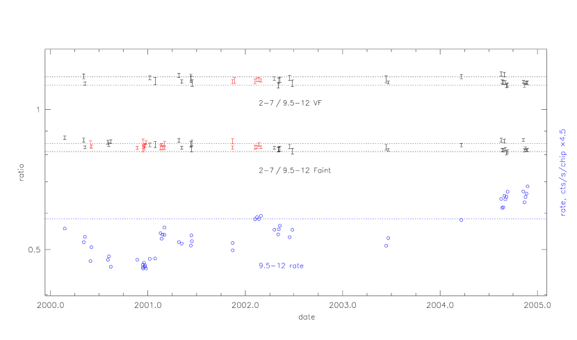
Figure 4.— Similar plot to Fig. 2 but for sky observations included in the blank-sky datasets, approximately corrected for the unresolved sky signal. The top points show the ratio with VF cleaning, the middle points with no VF cleaning, circles show the arbitrarily scaled 9.5–12 keV count rate. The pairs of dotted lines show $\pm$2% around the averages for 2001–2004. Dates of some points are shifted for clarity. Red points show the CDF observations. For CDF-N VF data, the ratios were corrected for the 1% effect of the upper 3025 ADU PHA cutoff (§ 3.3). Note that we use the energy range 9–12 keV for normalizing the background spectrum (§ 4.1.3), here we show the 9.5–12 keV band, for applicability to analysis of fields including brighter sources, which can have significant sky flux in the range 9–9.5 keV.

4.1.2 Constancy of the spectral shape

Another important fact seen from Fig. 2 is that while the total background rate is very different (lower data points), the ratios stay within a $\pm$2% rms, some of which is statistical scatter. The exception is an excess at $E<1$ keV from the dark Moon, which is an astrophysical signal (Wargelin et al., 2004). The same conclusion on the constancy of the background spectral shape within $\pm$2% rms was reached from looking at variability of the Event Histogram mode data (Markevitch et al., 2003).

The comparison of a larger number of sky observations included in the ACIS blank-sky background datasets, which span the 2000-2004 period, also shows an rms scatter of not more than 2% in the 2–7 keV to 9.5–12 keV background flux ratio (Fig. 4). The observations included in this plot are cleaned of background flares (using a less rigorous criterion than we will use in the work below, see § 4.2), and the detectable point sources are removed. Because of different exposures (30–160 ks), they include different contributions of unresolved CXB, which we approximately subtract using the results obtained in § 7.1 (Fig. 10) and assuming a uniform CXB over the sky, before dividing by the 9.5–12 keV rate. This correction is small in the 2–7 keV band but at lower energies the residual sky flux is too great, so we can only use these observations for checking the detector background variability at high energies. Most of the observations are in VF mode, so we show the ratios both for VF-cleaned and uncleaned (i.e., equivalent to F mode) data. Earlier observations were obtained in F mode so we cannot apply VF cleaning to them.

We note that VF-uncleaned ratios may show some downward trend during 2000 at a 2% level, which is probably related to the slowly changing CTI in the FI chips. The CTI and time-dependent gain corrections are calibrated for real X-ray photons registered in the imaging area of the CCD, and are not corrected for the undamaged frame store area of the CCD. For a fraction of the background that originates in frame store, these corrections result in energy shifts, thus we may expect apparent changes of spectral shape with time. The CDF-S and CDF-N F data were obtained during the above period of a possible trend. Our systematic uncertainty will include this, and we will see that the results are consistent within our systematic uncertainties between all datasets.

The VF cleaning removes a relatively larger fraction of the background events originating in frame store, thus reducing these time dependencies. Indeed, as seen in Fig. 4, the spectral shape of the VF-cleaned background does not show any trends with time; all ratios are within the 2% rms scatter. This is in contrast to the highly variable XMM-Newton background spectra (e.g., De Luca & Molendi, 2004; Nevalainen et al., 2005). Thus we are safe to use the 2002–2005 ACIS-stowed background to model CDF-N VF observations from the end of 2001 to early 2002. We will therefore treat the CDF-N VF subset as the most reliable for background-sensitive 2–8 keV measurements, although we will see that the other datasets give consistent results.

4.1.3 Background normalization

Since the Chandra effective area in the 9–12 keV band is negligible, essentially all the 9–12 keV flux in the sky data is due to particle background (in the absence of event pileup, which is true for all the CDF observations, see § 4.2.1). Because of the stability of the quiescent background spectral shape, we can therefore scale the normalization of the stowed spectrum to the observations by equating the 9–12 keV count rates, to get an accurate model of the non-sky quiescent background. In addition to the statistical uncertainty, we include a $\pm 2$% variation on this normalization to represent a systematic uncertainty of the background spectral shape inherent in such modeling, and propagate it into our final results. This variation is considered independent between the three CDF datasets because they are well separated in time (see Table 1), but is conservatively taken to be the same for observations within each dataset, which were usually taken back to back. This simple step is adequate and will be much more important for our 2–8 keV result than for the $E<2$ keV results. We note that this 2% background error may be somewhat conservative for the CDF-N VF data, since the shape of the VF background spectrum is very stable.

Figure 5.— 2.3–7.3 keV light curves for the CDF-N VF observations. Bins are 1 ks, count rate errors are shown at upper left. Dotted lines show the mean count rates after cleaning. Shaded bins are excluded by the combination of cleaning techniques described in § 4.2. Shaded intervals that are smaller than the 1 ks bins are due to gaps in good time intervals from standard processing.

Figure 5.— (contd), for the CDF-N F and CDF-S observations.

4.2. Flaring background

ACIS is also subject to background flares whose spectra are variable and different from that of the quiescent background. Because the present work relies on the accuracy of the background model at a 2–3% level, excluding these flares is the most critical aspect. We identify flares by their time and spectral variability. We create light curves for each observation in the 2.3–7.3 keV band, which is the most sensitive to flares due to the spectral shapes of the flaring and quiescent backgrounds (the quiescent background plus the sky signal has a minimum in this band, while the flares do not, see Fig. 3). For light curve extraction we include the whole ACIS-I array, but exclude the A03 point sources as described in § 3, although with exclusion radii 1/3 the size, so as to allow for greater background count rates and improved statistics. Three CDF-N observations (ObsIDs 2344, 3388, and 3389) were completely excluded from the spectral analysis because of extensive flaring activity.

For the remaining observations, we filter the light curves for flares successively in bins of 1 ks, 4 ks, and 10 ks, to try to balance the sensitivity to flares and statistical scatter. For each light curve we calculate a first approximation mean count rate, by rejecting bins with rate $>$3$\sigma$ over the mean from the full exposure. We then further exclude bins where the count rate deviates from this mean by 20%, 10%, and 6% for the 1 ks, 4 ks, and 10 ks binned light curves, respectively. This corresponds to 2$\sigma$ deviations for each binning, so we necessarily exclude some statistical devitions. We exclude both positive and negative deviations, even though the latter are mostly statistical fluctations, so as not to bias negatively the result by removing only positive statistical fluctuations.

Figure 6.— Ratio of 2.3–7.3 keV count rate to 9–12 keV count rate, in bins of 20 ks, for each observation. $\pm$1$\sigma$ errors are shown at upper left. Dotted lines show mean ratios after cleaning (note the difference between F and VF observations), dashed lines show $\pm$3 variations. Time bins excluded by this ratio cleaning are shaded, along with periods excluded by the standard processing (before our time filtering).

We also identify flares by using the fact that ACIS flares have different spectral shapes than the quiescent background. In particular, ACIS-I flares often have a power law spectrum with photon index $\sim$0 for $E>0.5$ keV, and weak or completely absent fluorescent lines. Thus for flares, the ratio of 2.3–7.3 keV flux to 9–12 flux will be systematically larger than for the quiescent background (Fig. 3). We therefore derive the ratio between the 2.3–7.3 keV and 9–12 keV count rates as a function of time in bins of 20 ks, and exclude periods with deviations of $>$3%, which corresponds to 1.5$\sigma$ statistical scatter. While the count-rate filtering is performed using individual mean values for each observation, for this spectral ratio filtering, we use a single mean value for the nominal ratio (separately for F and VF data, due to the different background levels). This ensures that across all observations the spectral shape is constant. This kind of filtering is well-suited to removing low-level flares and has not been performed before.

Because this ratio filtering includes the entire ACIS-I array and not just the central 5′, the problem of the upper telemetry cutoff in the CDF-N VF data (§ 4.1) becomes important, in that it may cause a higher 2.3–7.3 keV to 9–12 flux ratio in those observations with more missing photons having PHA_RO $>$ 3025. For the CDF-N VF data, we therefore performed the ratio filtering again, using the count rate for events with $E>9$ keV and PHA_RO $<$ 3025, which should not be affected by the telemetry cutoff. This check gives essentially identical output time intervals, and has negligible effect on the final spectrum.

Background light curves, showing the filtered time intervals, are shown in Figs. 5–6. The above filtering steps, applied separately, exclude 12%, 14%, 18%, and 24% of the exposure time for the 1 ks, 4 ks, and 10 ks light curve and 20 ks flux ratio cleaning, respectively (note that with the larger binning, we necessarily exclude some time intervals at the start or end of each observation that are not included in bins). After combining these filters a total of 32% of the exposure time is excluded (39% if we include the three observations that are completely excluded due to flares). This is a much more rigorous cleaning than normally applied for the ACIS-I extended-source data (which is limited to our 1ks, 20% light curve cleaning step, and on average removes 6% of the total exposure, e.g., Vikhlinin et al., 2005), and is sufficient to remove flaring intervals to our required accuracy.

4.2.1 ACIS-I readout artifacts

A small but significant contribution to the background comes from the 41 ms of time needed to read out the CCD, for each sky exposure of 3.1 or 3.2 s (3.1 s for the majority of the CDF observations). This leads to artifacts in the forms of streaks along the CHIPY direction accompanying all celestial sources. Because these events lie outside the source exclusion regions, we simulate and remove this readout background using the make_readout_bg routine (Markevitch et al., 2000). This script takes the original event list and randomizes the CHIPY values for each event, then recalculates the photon energies to produce a new event list which approximately simulates the spectral and spatial characteristics of the readout artifact. The method works only when there is no pileup in the observations. This is true for both CDF fields; the very brightest sources in the A03 catalog have count rates 0.022 (CDF-N) and 0.012 (CDF-S) counts s^-1, for which pileup will be $<$3%.

Using this readout event list, we extract a spectrum (hereafter the ”readout spectrum”) using the same GTI and region filters as for the sky events. During spectral fitting, we subtract the readout spectrum with a normalization of $0.0132=41\>\rm{ms}/3.1\>s$. This also subtracts a fraction of the detector background, which is taken into account when normalizing the stowed dataset.

To summarize, the unresolved sky spectrum is given by

$$f_{\rm unr}=f_{\rm obs}-C_{\rm bg}f_{\rm stowed}-0.0132f_{\rm readout}.$$ (2)

where $f_{\rm obs}$ is the observed spectrum with sources excluded, and $C_{\rm bg}$ is the stowed background scaling factor, given by

$$C_{\rm bg}=\frac{f_{\rm{9-12\>keV}\>(obs)}-0.0132f_{\rm{9-12\>keV}(readout)}}{f_{\rm{9-12\>keV}(stowed)}}.$$ (3)

By design, this subtraction gives zero flux at 9–12 keV.

5. Spectral extraction

For each observation, we extract source-excluded spectra of the sky, using the region and time filters described above, specific to each observation. Due to differences in pointings of up to 4′, the exposures in a given field (and our $r<5$′ extraction regions) have slightly different sky coverages. Our analysis implicitly assumes that across the different pointings in a given field, the faint, unresolved sky signal has the same surface brightness.

For each CDF exposure, we project the stowed events into sky coordinates using the appropriate aspect solution, using the make_acisbg routine (Markevitch et al., 2000). We then extract a spectrum (hereafter called the ”stowed spectrum”) using the same region filtering as for the sky exposures. The normalization of the background spectrum is described in § 4.1.3.

For any individual observation, the unresolved signal is too faint for detailed spectral analysis. Therefore we created composite spectra for each of the three subsets of the data, CDF-N VF, CDF-N F, and CDF-S. The RMFs and ARFs are derived using A. Vikhlinin’s ACIS tools CALCRMF and CALCARF. These are equivalent to the standard CIAO tools, except that CALCARF also includes an area-dependent dead-time correction (a 3% effect). In each observation, RMFs and ARFs are averaged over the extraction region. Between observations, RMFs and ARFs are averaged by exposure time, using the FTOOLS addrmf and addarf. The stowed spectra are also averaged, weighted by the corresponding sky exposure time. Note that even though the same stowed background dataset is used for all observations, the sky coverage is slightly different, which results in small differences in the stowed background spectra. Care is taken to treat the background data in a statistically correct way, and not as independent spectra. We also approximately take into account the fact that the I0 and I1 stowed data are not independent (§ 4.1). Of the background events 12% (CDF-N) and 22% (CDF-S) are taken from the I1 chip. We thus increase the statistical errors on the background spectrum accordingly, by 7% for CDF-N and 13% for CDF-S. The 2% systematic normalization uncertainty (§ 4.1) is conservatively applied to the combined stowed spectrum for each dataset.

5.1. ACIS calibration

The latest calibration is used as described in Vikhlinin et al. (2005). The data processing used the CTI correction CALDB file ctiN0002, ACIS gain file gain_ctiN0003, and time-dependent gain correction t_gainN0003, the same versions as used for stowed data (the recently released updates do not affect our results significantly). The instrument responses included time- and position-dependent low-energy contamination correction (equivalent to the CALDB file contamN0004), mirror edge correction function applied to the CALDB effective area file axeffaN0006, which is equivalent to using the recently released updated area axeffaN0007, and the dead area correction to the FI quantum efficiency (QE) by a position-dependent factor around 0.97.

Because of these calibration updates, our absolute fluxes will be slightly different from earlier Chandra papers. In particular, because of the combined effect of mirror area, dead time and position-dependent contaminant corrections, our 1–2 keV fluxes should be within 2–3% of those in A03, but lower by about 5–7% at 2–8 keV. The ACIS-S measurement by Markevitch et al. (2003) was additionally affected by old values of the uncontaminated low-energy QE for BI chips (not used here), resulting in an overall 7% overestimate of the 1–2 keV fluxes. It is difficult to evaluate the differences with still earlier analyses, e.g., of M03.

6. Results

Composite spectra of the unresolved CXB are shown in Figs. 7–9. There is significant flux below $\sim$2 keV, consisting of two components: the diffuse soft background, likely a combination of the Galactic Local Bubble emission (Snowden, 2004) and charge exchange emission in regions local to the Sun (e.g., Cravens, 2000; Wargelin et al., 2004), as well as residual flux from unresolved X-ray point sources and possibly other CXB components. The soft diffuse flux consists mainly of oxygen lines and can be modeled as a thin-thermal plasma (the APEC model Smith et al., 2001) with $kT\sim 0.15$ keV, solar abundances, and zero interstellar absorption, as in other regions of the sky away from Galactic features (e.g., Markevitch et al., 2003). The remaining flux can be modeled as a power law with a Galactic absorbing column (1.5 and $0.9\times 10^{20}$ cm^-2 for CDF-N and CDF-S, respectively, Dickey & Lockman, 1990).

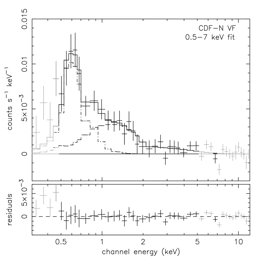
Figure 7.— Unresolved, background-subtracted sky spectrum for the composite CDF-N VF data. The fit was performed in the energy range 0.5-7 keV (excluding 5.6–6.2 keV) and consists of a power law and APEC components, shown as dashed lines. We show the whole range from 0.3–12 keV for completeness; bins not included in the fit are in gray. Fit results are given in Table 2.

We first fit the spectra in the range 0.5–7.3 keV. The upper cutoff here is to avoid bright background lines which appear at $E>7.3$ keV (Fig. 3). We also exclude bins between 5.6–6.2 keV, to avoid a faint Mn K$\alpha$ line that apparently makes its way from the calibration source inside the detector housing. Because this radioactive source decays with time, and because the line brightness at the ACIS-stowed position may be different from that in the normal position, this line may be subtracted incorrectly when using the stowed background. Most other bright background lines are above our 7.3 keV upper cutoff. For the flux calculations, we also exclude the 2.0–2.3 keV interval to avoid a bright Au line in the detector background; although it does not affect the fits, it does add to errors when the background normalization is varied. Hereafter the spectral analysis and count rates exclude these line intervals, although the model fluxes are calculated including them.

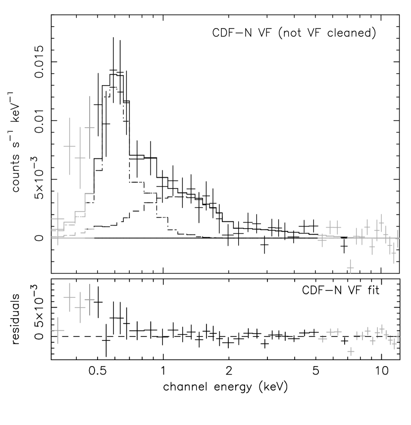
Figure 8.— Same as Fig. 7, but for the CDF-N VF data with no VF cleaning. The best fit model to the CDF-N VF spectrum and its residuals are shown, indicating a good fit for $E>0.7$ keV.

Fitting results are given in Table 2. For our best dataset, the CDF-N VF spectrum, a combination of the thermal model plus power law produces a good fit in the 0.5–7.3 keV band, giving $kT_{\rm APEC}=0.18$ keV and $\Gamma=1.5$. The thermal component dominates at $E\lesssim 0.8$ keV. There is some excess above this model for $E<0.5$ keV (outside our fitting range), which is not surprising because a single-component APEC model may not be a complete, nor even physical, characterization of the diffuse soft background (e.g., Markevitch et al., 2003; Wargelin et al., 2004). However the APEC model is sufficient for our purposes, and gives a very small contribution at $E>1$ keV.

To check that we can compare our fit results for VF-cleaned data to F mode data, we created a composite spectrum, as above, for the CDF-N VF subset, but without the VF cleaning. This spectrum gives very similar spectral parameters to the VF-cleaned data. The spectrum is shown in Fig. 8 with residuals from the best-fit model for the VF-cleaned spectrum. There is only a small excess above the model for $E=0.5$–0.7 keV (where VF cleaning removes a large fraction of background events), but above 1 keV the results are essentially identical.

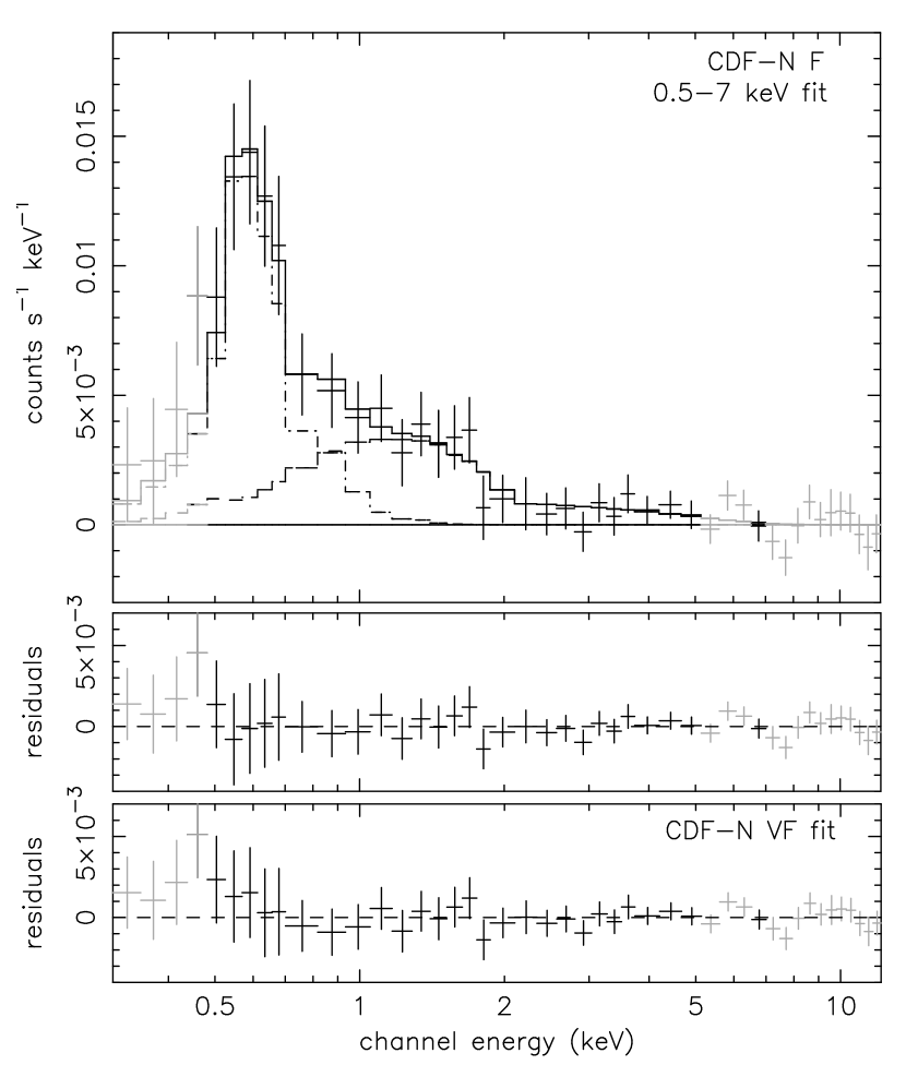
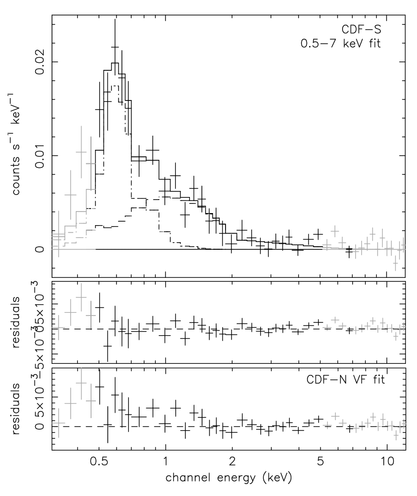
Figure 9.— Same as Fig. 7, but for F mode composite spectra for (a) CDF-N and (b) CDF-S. Fit results are given in Table 2. Residuals from the best-fit CDF-N VF model are shown at bottom.

The composite CDF-N F and CDF-S spectra give best-fit spectral parameters that are consistent with the CDF-N VF results (Table 2), even though the CDF-S field is half the sky away and was taken one year earlier. The spectra are shown in Fig. 9, along with residuals to the best-fit CDF-N VF model. The CDF-S spectrum has a somewhat steeper best-fit power law slope ($\Gamma=1.8$) and correspondingly higher normalization, both within 1–2$\sigma$ of the CDF-N VF fits. It is well-fit by a $\Gamma=1.5$ power law above 2 keV.

Table 2Fits to composite spectra

Parameter	CDF-N VF	CDF-N F	CDF-S
$N_{H}$ ($10^{20}$ cm-2)	1.5	1.5	0.9
Background (0.5–7.3 keV fit)
power law $\Gamma$	$1.48_{-0.38}^{+0.46}$	$1.41_{-0.37}^{+0.43}$	$1.84_{-0.35}^{+0.48}$
$I_{\rm PL}$	$2.3\pm 0.5$	$2.3_{-0.5}^{+0.5}$	$3.3\pm 0.6$
$kT_{\rm APEC}$ (keV)	$0.177_{-0.016}^{+0.010}$	$0.162_{-0.017}^{+0.015}$	$0.175_{-0.019}^{+0.010}$
$I_{\rm APEC}$	$3.4_{-0.4}^{+0.7}$	$3.7_{-0.7}^{+1.2}$	$4.0_{-0.5}^{+1.0}$
Point sources
power law $\Gamma$	$1.39\pm 0.03$		$1.47\pm 0.04$
$I_{\rm PL}$	$7.00\pm 0.15$		$6.78\pm 0.18$

For each composite spectrum, we calculate the total observed flux in the 0.5–1 keV and 0.5–2 keV bands. For 0.5–1 keV, the power law contributes 15% of the flux for both CDF-N spectra, and 20% for CDF-S. We also calculate unabsorbed fluxes in the extragalactic (power law) component for 1–2 keV (with its extrapolation to 0.5–2 keV) and 2–8 keV, performing separate fits for each energy band to minimize their model dependencies. Because of the limited number of counts, the fits in these bands do not tightly constrain the power law slope, which strongly affects the output flux in energy units in the 2–8 keV band. Therefore, we fix $\Gamma$ and vary only the normalization; from each best fit model we calculate the observed flux. For simplicity, we use values of $\Gamma$ over the 1$\sigma$ errors of the CDF-N VF 0.5–7.3 keV fit (1.1, 1.5, 2.0). For our final results we will use $\Gamma=1.5$, and will fold into the uncertainty the variations in calculated flux between $\Gamma=1.1$ and 2. We note that although the CDF-S spectrum has a best-fit $\Gamma=1.8$, for 0.5–7.3 keV, we do not introduce a significant error into the flux values because we fit the spectrum normalization separately in the individual bands. For all wide-band flux measurements in this paper, we include an ACIS flux calibration uncertainty of 3%.

6.1. PSF scattering

While we have used large exclusion regions to remove the contribution of point sources, a small fraction of the source counts, in the wings of the PSF, will not be excluded and must be subtracted from our unresolved fluxes. To estimate this scattered flux we use a model (from the Chandra CALDB) which gives the shape of the ACIS PSF as a function of energy and off-axis angle. Using the A03 catalogs for CDF-N and CDF-S sources, we calculate the PSF for each source inside the 5′ extraction radii. We thus determine the total count rate for scattered source photons that are outside the exclusion regions. We find that in the 1–2 keV band, 1% (CDF-N) and 0.5% (CDF-S) of the unresolved fluxes come from scattered source photons. For 2–8 keV, where the PSF is broader, this fraction is 4% for CDF-N and 2% for CDF-S. Hereafter, unresolved fluxes have been corrected by these factors.

Table 3Unresolved fluxes from composite spectral fits

	CDF-N VF	CDF-N F	CDF-S	Average
Observed (power law + APEC)
0.5–1 keV	$4.0\pm 0.3$	$4.3\pm 0.5$	$5.0\pm 0.4$	$\cdots$
0.5–2 keV	$4.9\pm 0.6$	$5.3\pm 0.6$	$6.0\pm 0.5$	$\cdots$
Extragalactic (unabsorbed power law)
0.5–2 keV	$1.58\pm 0.34$	$1.68\pm 0.39$	$2.05\pm 0.41$	$1.77\pm 0.31$
1–2 keV	$0.93\pm 0.17$	$0.99\pm 0.20$	$1.20\pm 0.19$	$1.04\pm 0.14$
2–8 keV	$3.5\pm 2.4$	$3.1\pm 2.4$	$3.6\pm 2.2$	$3.4\pm 1.7$

Note. — Intensites are in units of $10^{-12}$ ergs cm^-2 s^-1 deg^-2.

6.2. Calculation of background intensity

To convert the unresolved flux into intensity, or sky surface brightness, we divide the observed flux by the effective solid angle subtended on the sky by the extraction region. To find this solid angle, we create an exposure map for the ACIS-I array for each observation, normalized to a maximum value of 1. We do not include the effects of the mirror vignetting and CCD efficiences, as these are included in the ARF during the flux calculations, so that only the chip coverage, the excluded columns on the CCDs, and the telescope dither are included in the image. We then integrate this image within the sky spectrum extraction regions (described in § 3), to give the effective solid angle for the unresolved spectrum. For the composite spectra, we average these solid angles weighted by the exposure time of each observation, giving 0.0135 deg² for both CDF-N VF and F, and 0.0159 deg² for CDF-S. These are used to calculate the unresolved background intensities, which are given in Table 3.

For measuring the intensity due to sources (see § 8.2.1), we perform a similar solid angle calculation, including the chip coverage and telescope dither, for the entire central 5′ region (without the exclusion regions). The exposure weighted averages of these solid angles are 0.0202 deg^-2 for CDF-N and 0.0200 deg^-2 for CDF-S.

6.3. Average unresolved intensities

Under the assumption that the unresolved CXB is isotropic, we calculate mean values of the unresolved CXB intensity using measurements from the three data subsets. We take care to treat the statistical errors in the stowed background dataset (which comprise $\sim$40% of the total error) as not independent between the subsets. We therefore average only those errors that arise from statistics in the observed sky count rates, and in the 2% uncertainty in the detector background shape (which should be independent for the three subsets, which are separated in time by $\sim$1 year). Mean values for the unresolved intensities are given in Table 3. Details of the error propagation is shown in Table 4, which is described in detail in § 8.2.3.

7. Verification

In this section we test the dependence of our measurement on the details of the source exclusion and background modeling, and also consider the possibility of residual background flares significantly contaminating the unresolved signal.

7.1. Contribution from fainter sources

The source catalog from A03 that we use here was derived with completeness in mind, and so was limited to sources brighter than a certain flux. We test here whether fainter but still detectable sources contribute significantly to the observed signal. To detect sources at lower significance than A03, we use all the CDF exposures (including those before 2000 January 21, see A03, Table 1 and A1 for full lists) to create a deep image for each field (Fig. 1). After a less conservative cleaning for bright flares, these images have exposure times of 1.9 Ms for CDF-N and 0.8 Ms for CDF-S. We detect sources in three bands, 0.5–2, 2–8, and 0.5–8 keV, corresponding to the “soft”, “hard”, and “full” bands of A03. We run the wavelet decomposition (Vikhlinin et al., 1998) on these deep exposures, and measure centroids and fluxes using the largest-scale wavelet decomposition as the background. For source exclusion purposes, it is not necessary to match the sources detected in different bands, even though the source exclusion regions will overlap. Our detected source list therefore consists of a concatenation of the sources detected in the individual bands.

Figure 10.— Unresolved CXB intensity, excluding sources with different minimum numbers of counts in the 0.5–8 keV band. Open symbols are for 1–2 keV, filled symbols are for 2.3–7.3 keV. Errors are not shown for clarity. The differences between the fields are within their statistical uncertainties. Note that the slight upturn at 2 counts per source for CDF-N VF 2.3–7.3 keV is not significant. The increase in intensity is due to the smaller solid angle over which the unresolved flux was calculated.

We sort the detected point sources by the number of photons associated with each source (total photons minus background) for the 0.5–8 keV band. We then extract the unresolved spectrum (for CDF-N VF and CDF-S), after excluding sources with different minimum numbers of photons. In the A03 catalog, the minimum number of detected photons was 11.4 for CDF-N and 8.0 for CDF-S. However for our test we have detected sources at very low significance down to 2 photons above the background. By excluding the contributions of these possible sources as well, we can determine if such low-flux objects contribute significantly to the total flux.

In Fig. 10 we show the unresolved intensity, as a function of the minimum number of counts from excluded sources. It is apparent that sources with 2–10 source photons do not contribute significantly to the background flux. We note that while many of these fainter “sources” are not real and are only due to statistical fluctuations, any real sources are detected and excluded. This confirms that our results are insensitive to the details of source detection.

We also have directly checked that we are fully excluding scattered flux from sources, by re-calculating the unresolved CXB intensities using exclusion radii that are 30% larger for point sources, and twice as large for extended sources. We find that the results agree to $\lesssim$3%, as expected (§ 6.1).

7.2. Variations in I1 chip

Because the stowed observations did not include the I1 chip (which is modeled using the events from the I0 chip), it is possible that the stowed background spectrum is somewhat different for this chip and thus is not properly subtracted in our analysis. We have tested this by performing the spectral analysis including only chips I0, I2, and I3, and find no changes in the unresolved intensities and spectral parameters to $<$2%. Therefore the I1 chip background subtraction has negligible effect on the results.

7.3. Contributions from flares?

Because of the very small unresolved signal, even a very low-level residual background flare contribution can affect our results. The 2–8 keV count rate for the instrumental background is a factor of $\sim$25 larger than that for our unresolved sky signal, so even a flare on the level of a few percent can have a significant effect. Therefore it is important to rule out the existence of such low-level flares.

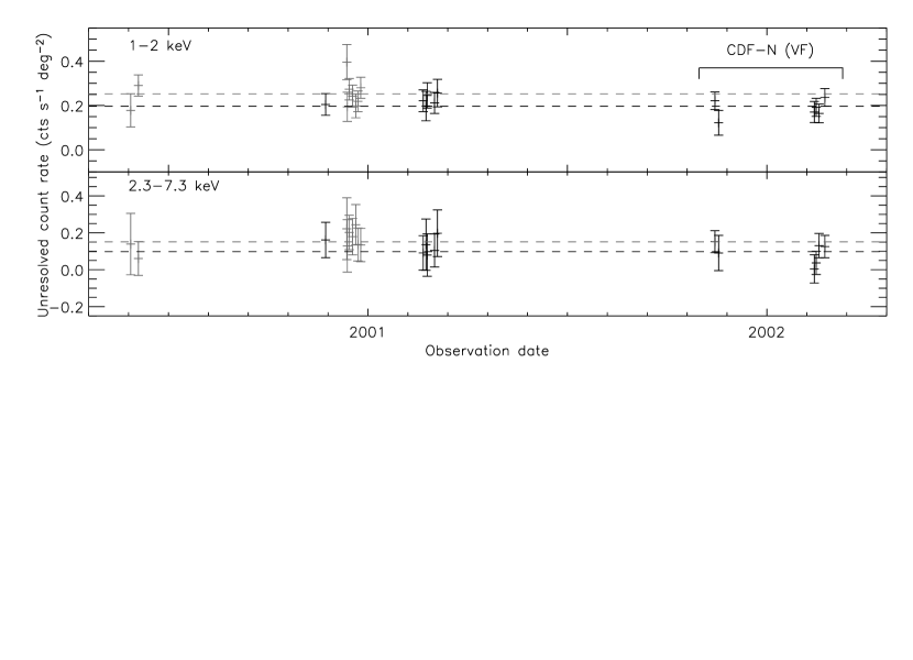
Figure 11.— Points with error bars show the unresolved CXB intensity in the range 1–2 keV (top) and 2.3–7.3 keV (bottom), for 21 CDF observations that are included in the spectral analysis (CDF-N in black, CDF-S in gray). Shown with dashed lines is the count rate for the composite CDF-N VF and CDF-S observations.

We first test for flares by directly examining the observed unresolved spectrum. Fig. 3 shows a sum of several observed flares in ACIS-I spanning a number of years and an order of magnitude in intensity, giving a representative average flare spectrum that we could possibly expect in our long datasets. A spectrum from the quiescent periods was subtracted for each included observation, so only the flare excess is shown. The individual flares have similar (although not identical) general spectral shape, regardless of the brightness; the relative intensity of the fluorescent lines, if present, varies from flare to flare (always being lower than in the quiescent spectrum). The flare spectrum in Fig. 3 is normalized to have the same 9–12 keV rate as the quiescent spectrum. Clearly, it has a shape that is very different from the quiescent background, and from the shape of the much more frequent BI-only flares (Markevitch et al., 2003). What is most useful for us is that the flares are also very different from the X-ray sky signal, increasing steeply towards low energies where the sky spectrum is absorbed by the CCD filter. We can therefore use spectra at low energies to put constraints on flare contamination.

When the normalized quiescent background is subtracted from the flare spectrum in Fig. 3 (as it would be in our analysis if it were present in a sky spectrum), its spectrum in the 0.3–7 keV band, excluding the 1.8–2.2 keV line interval, can be described (without the application of an ARF) as a sum of two power laws, with soft $\Gamma=1.7$ and hard $\Gamma=-0.1$, with a 13% contribution of the soft component to the total 0.3–7 keV count rate.

We fit the unresolved spectra, including such a flare model, in the 0.3–7 keV band. We add the two power law model above, fitted with no ARF, to the same APEC plus power law spectrum as in § 5. For all three composite spectra, we find that the flare component can contribute at most $\sim$14% of the flux (1$\sigma$ upper limit) in the 1–2 keV band and $\sim$35% in the 2–8 keV band. The addition of this flare model does not significantly improve the reduced $\chi^{2}$ of the fit.

We should note that a different, very rare FI flare species was observed, consisting mostly of the high-energy fluorescent lines, but it could not significantly affect our results due to its spectral shape.

We can also test for flares by noting that flare activity is generally time-variable and so might be expected to give a strong variation in the background-subtracted count rates between observations. To check this, we subtract background as described in § 4 for each of the individual exposures, and calculate a count rate scaled by the effective solid angle on the sky (see § 6.2), for the 1–2 keV and 2.3–7.3 keV bands, shown in Fig. 11. Errors include the statistical count rate uncertainty, as well as the statistical uncertainty in the background normalization (but not its systematic uncertainty). In both bands, the count rates over time are consistent with those from the CDF-N and CDF-S composite spectra. Note that because we normalize the quiescent background using the 9–12 keV count rate, our filtering using the ratio of the 2.3–7.3 keV and 9–12 keV count rates (§ 4.2) should make, by design, the residual 2.3–7.3 count rates equal to within the statistical errors. The larger statistical scatter is due to the fact that the ratio filtering was performed on the full ACIS-I field, whereas here the fluxes are from the $r<5$′ region, which is 5 times smaller. We stress, however, that we have not performed any light curve filtering using the 1–2 keV band, so the fact that the 1–2 keV signal is not dominated by a few bright observations implies that there is no significant flare contribution.

Thus, any flare contribution could only be due to some low-level, persistent background flare that is roughly constant over many observations spanning several years. One could possibly argue that our filtering selects a low-end tail of the flare distribution, but this is not the case. Recall that 20 ks bins with spectral deviations outside 3% from the global average were excluded during the temporal cleaning (§ 4.2). This filtering excludes 24% of the total exposure, but most of these excluded deviations are quite small; in fact, only two (for ObsIDs 3294 and 3390) appear to be inconsistent with purely statistical scatter. (Fig. 6). We note as well that the blank sky observations shown in Fig. 4 have not been filtered using the band ratio as we did here, and they still show a rather constant flux in the 2–7 keV band over several years. We conclude that any significant flare contamination is very unlikely. We also remind here that there is no constant background component that is present in the sky data but absent in the stowed background, as shown by comparison of the stowed and dark Moon observations (§ 4.1.1).

8. Discussion

8.1. Comparison between datsets

The unresolved CXB intensities (Table 3) are consistent to 1$\sigma$ for the three datasets; the difference between CDF-N and CDF-S is $<$25%. We note that although the source detection limits in these two fields are different by a factor of two, the contribution of sources with fluxes between these limits is relatively small. Given typical $\log{N}/\log{S}$ distributions (see § 8.2.2 M03), sources between the two flux limits should only contribute $\sim$$6\times 10^{-14}$ ergs cm^-2 s^-1 deg^-2 for 1–2 keV and $3\times 10^{-13}$ ergs cm^-2 s^-1 deg^-2 for 2–8 keV, which are small compared to the unresolved fluxes and our measurement errors. Although we cannot make definitive statements using only two fields, this correspondence between CDF-N and CDF-S hints that the distribution of X-ray sources at fluxes below the current detection limits (or any diffuse component) is isotropic. This is especially interesting given that the CDF-S contains significantly fewer detected point sources (e.g., Brandt et al., 2001a; Rosati et al., 2002).

8.2. Total X-ray background

To compare our results to other studies, we determine the total X-ray background intensity in the ranges 1–2 and 2–8 keV, by adding our measured signal to flux from detected sources from the CDF observations and from wider-field surveys. We can then use the total CXB value to obtain the resolved fraction of the CXB. We note, however, that it is the absolute unresolved flux given above, not the resolved fraction, that usually matters for source population studies.

8.2.1 Spectra of the excluded sources

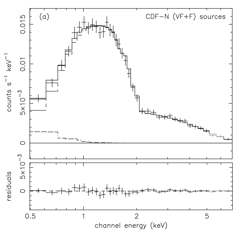
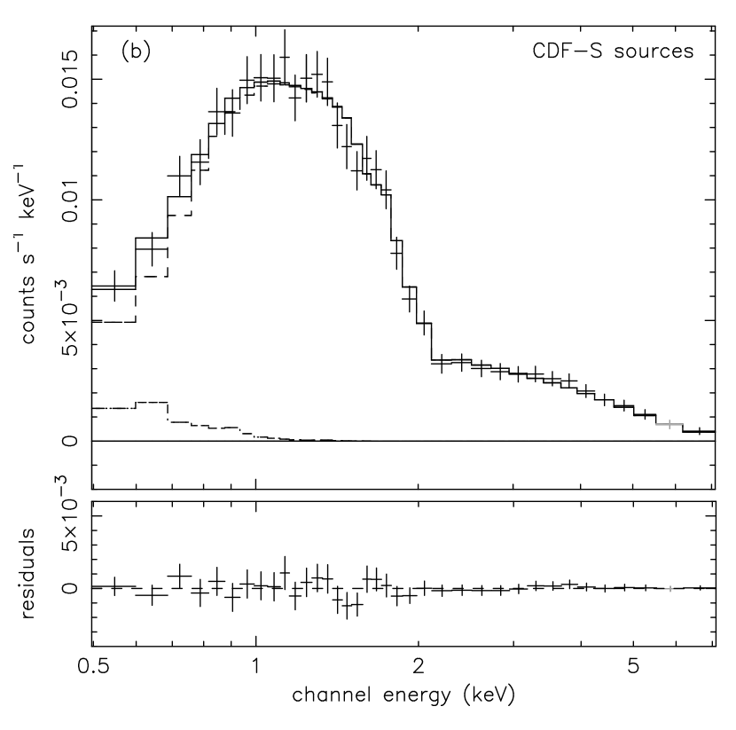
Figure 12.— Total spectra for detected sources from the A03 catalog contained within 5′ radius of the aimpoint for any observation, for the (a) combined CDF-N (VF + F) and (b) CDF-S datasets. The separate APEC and power law components are shown as dashed lines. Spectral fits are given in Table 2.

Figure 13.— Variation in power law photon index $\Gamma$ with source flux, for (a) 0.5–2 keV and (b) 2–10 keV sources. Data for 0.5–2 keV are from the ROSAT study of Vikhlinin et al. (1995b), for 2–8 keV data are from ASCA (stars della Ceca et al., 1999) and CDF-S (crosses Rosati et al., 2002). In both cases the flux dependence of $\Gamma$ is fit with a scaled error function (solid lines).

First, we extract the total spectrum of the detected point sources for each of the two fields. To limit the effects of vignetting, for each individual observation we only include sources from inside the 5′ radius. Because there are variations in the pointing between the observations (especially for CDF-N), the 5′ circle covers slightly different patches of sky for each observation. Thus the total solid angle sampled is 0.0331 deg^-2 for CDF-N and 0.0237 deg^-2 for CDF-S. However, each individual spectrum covers only the central 5′ circle, so when we add the spectra, the effective sky coverage of the total spectrum is an exposure-weighted mean of the sky coverages of the individual 5′ regions. Therefore, we use the solid angles as given in § 6.2 to calculate the total source flux deg^-2.

Figure 14.— Measured and total (including bright source correction) fluxes for our composite source spectra, as a function of the upper flux cutoff (§ 8.2.2) for (a) CDF-N and (b) CDF-S. Fluxes for sources in the soft band are given for 0.5–2 keV, while total intensities are for 1–2 keV. Errors shown on the total fluxes include measurement error and Poisson error in both the measured source fluxes and in the bright source correction.

Figure 15.— Measurements of the total (a) 1–2 keV and (b) 2–8 keV CXB. For our results, the relative contributions of sources from CDF-N and CDF-S are shown as two separate crosses; the totals are calculated from the average of these. Our measured unresolved intensities are shown by brackets. The small error bar on our total CXB represents only the error in the unresolved component. Full error bars, including uncertainty in bright source corrections, are shown just to the right. References marked with an asterisk have been corrected for the contributions of bright sources (Table 6). Note that these values are somewhat different from a similar plot in M03.

We extract the source spectra in regions as described in § 3.2, although with a smaller radius of $1.5r_{90}$ for each source, so as to include most source flux but to limit the diffuse background contribution. Composite spectra for CDF-N (combining F and VF) and CDF-S are shown in Fig. 12. We fit the spectra with the APEC plus a power law component. The APEC model is necessary because the source extraction regions still have sufficent area to detect the soft diffuse component; fit results are given in Table 2.

To calculate the total source intensities, we must perform aperture corrections to account for small amounts of scattered flux outside the extraction region. We use the A03 catalogs and the ACIS PSF model as described in § 6.1, and find aperture corrections of 5% (CDF-N) and 3% (CDF-S) for the 1–2 keV band, and 9% (CDF-N) and 6% (CDF-S) for the 2–8 keV band. The aperture-corrected source intensities in two bands are given in Table 5. The brightest sources in these fields have 0.5–8 keV fluxes of $3.5\times 10^{-14}$ and $1.1\times 10^{-13}$ ergs cm^-2 s^-1 for CDF-N and CDF-S respectively, and the lowest fluxes are at the A03 source detection limits (A03).

8.2.2 Total background using $\log{N}/\log{S}$

We cannot directly use the source fluxes determined above for CDF-N and CDF-S to determine the total background, because the narrow CDF fields do not include a representative number of bright, rare sources that contribute a significant fraction of the total. We must include their contribution based on source counts from published wider-area surveys. Furthermore, to reduce the effective Poisson scatter of the number of the rarest sources in our fields, we should remove the sources brighter than a certain flux (Hasinger, 1996; Lumb et al., 2002) which we will determine below.

In the soft band, Vikhlinin et al. (1995b) obtained a 0.5–2 keV $\log{N}/\log{S}$ curve from a wide-area (20 deg²) ROSAT PSPC survey for sources with fluxes between $1.2\times 10^{-15}$ and $7\times 10^{-13}$ ergs cm^-2 s^-1. We can directly use these data to interpret the Chandra results, since the most recent Chandra calibration shows negligible cross-calibration flux difference for ROSAT PSPC data (Vikhlinin et al., 2005). For the hard band, no single instrument has measured the range of fluxes necessary for this calculation. We instead use the M03 composite $\log{N}/\log{S}$ curve for 2–10 keV, which uses bright-source data from XMM-Newton and ASCA with a total survey area of 71 deg^-2.

Because these $\log{N}/\log{S}$ curves are for 0.5–2 keV and 2–10 keV, but we wish to calculate intensities for 1–2 keV and 2–8 keV, we need to determine how the source spectra vary with flux. Following the approach of M03, we use a smooth function to approximate the dependence of $\Gamma$ with flux. We use data obtained with ROSAT (Vikhlinin et al., 1995a) for the soft band (excluding stars which give a negligible contribution), and ASCA (della Ceca et al., 1999) and Chandra (Rosati et al., 2002) for the hard band (Fig. 13), and fit them with a scaled error function,

$$\Gamma(s)=a_{0}+a_{1}{\rm erf}\left(\log{\frac{S-a_{2}}{a_{3}}}\right)$$ (4)

where $S$ is in units of $10^{-15}$ ergs cm^-2 s^-1. For the fits we disregard the different error bars on each data point to avoid biases. The best-fit parameter values are $(a_{0},a_{1},a_{2},a_{3})=(0.59,1.7,-4.6,2.0)$ for 0.5–2 keV and $(-16,18,-12,0.41)$ for 2–10 keV. Fig. 13 shows these fits; the results will not depend significantly on the details of this approximation.

As mentioned above, we now integrate the sources detected in CDF up to a certain cutoff flux, after which we integrate the $\log{N}/\log{S}$ from wider-area surveys. For our purposes, the optimum upper flux cutoff should be high enough so that we measure as much of the CXB signal as possible using the CDF data itself (minimizing any cross-calibration error), but low enough to limit the shot noise from our bright sources. Using the total sky coverage of each field (§ 8.2.1) and using the above $\log{N}/\log{S}$ curves, we find optimum flux cutoffs of $5\times 10^{-15}$ ergs cm^-2 s^-1 for 0.5–2 keV sources and $1.4\times 10^{-14}$ ergs cm^-2 s^-1 for 2–8 keV sources. These give Poisson errors corresponding to $\sim$5% of the total CXB for the 1–2 and 2–8 keV bands, and still allow us to measure $\sim$50–60% of the total CXB using CDF data.

These cutoffs exclude several bright sources in each field. We exclude 5 sources in CDF-N and 4 in CDF-S for 0.5–2 keV, and 3 in CDF-N and 2 in CDF-S for 2–8 keV. The total aperture-corrected fluxes of the sources fainter than these cutoffs, divided by the solid angle of our $r=5$′ regions (see § 6.2) are given in Table 5. The CDF-S source intensity is $\sim$30% lower than that for CDF-N, consistent with the observed differences in the $\log{N}/\log{S}$ curves for those fields (e.g., Brandt et al., 2001a; Rosati et al., 2002).

The next step is to obtain the background intensity for sources brighter than our flux cutoffs, using the $\log{N}/\log{S}$ distributions of Vikhlinin et al. (1995b) and M03, and the $\Gamma$ as a function of flux shown in Fig. 13. Table 5 gives these total intensities, integrated to a maximum flux of $10^{-11}$ ergs cm^-2 s^-1 in the 0.5–2 keV and 2–10 keV bands. There is very little contribution ($<0.3$%) from still brighter sources. For the purposes of obtaining a total CXB value, we average the resolved intensities from these two fields.

To find the statistical errors in the bright source corrections, for each energy band we calculate the total number of sources in bins of flux, given the $\log{N}/\log{S}$ curve and survey area. The statistical errors quoted in Table 5 are simply the total Poisson uncertainties in these source counts. For bright source corrections we also include include an additional error of $\pm$5% to account for any cross-calibration uncertainties, as in DM04.

To verify that the total CXB value does not depend significantly on the value of the flux cutoff, we measure the aperture-corrected intensity of the combined source spectrum, plus the above bright-source correction, for several flux cutoffs above our optiumum values. These intensities are shown in Fig. 14. The errors shown include the measurement error on the fluxes, as well as the Poisson error in the measured fluxes and the bright source correction. Fig. 14 shows that the total flux varies as bright sources are included in the CDF spectrum, however these differences are always within the errors. Fig. 14 also shows that the errors on the total CXB with the increasing cutoff.

Table 4Summary of errors in unresolved intensity

		Count rate error		BG normalization error			PL $\Gamma$	Calibration	Total
Subset	Intensity	Sky	BG	Systematic	Sky	BG	error	error	error
(1)	(2)	(3)	(4)	(5)	(6)	(7)	(8)	(9)	(10)
1–2 keV
CDF-N VF	0.93	0.063	0.09	0.09	0.028	0.041	0.018	0.028	0.17
CDF-N F	0.99	0.074	0.10	0.12	0.029	0.040	0.020	0.030	0.20
CDF-N S	1.20	0.062	0.10	0.11	0.027	0.038	0.014	0.036	0.19
Average	1.04	0.039	0.10	0.06	0.016	0.040	0.017	0.031	0.14
2–8 keV
CDF-N VF	3.52	0.61	0.95	1.72	0.52	0.78	0.49	0.11	2.43
CDF-N F	3.05	0.61	0.92	1.73	0.52	0.78	0.50	0.09	2.37
CDF-N S	3.58	0.50	0.87	1.63	0.49	0.73	0.58	0.11	2.24
Average	3.39	0.33	0.91	0.98	0.29	0.76	0.53	0.10	1.69

Note. — Table columns are described in detail in § 8.2.3.

Together with our unresolved and resolved CDF fluxes, we use these bright source corrections to calculate total CXB intensities averaged across the fields, which are given in Table 5. These totals correspond to a CXB power law normalization (for $\Gamma=1.4$) of 10.9 photons cm^-2 s^-1 keV^-1 sr^-1 at 1 keV, and resolved fractions of $77\pm 3$% for 1–2 keV and $80\pm 8$% for 2–8 keV. We note that our resolved fractions are somewhat lower than those determined by M03, who used similar values for the total CXB from the literature but found higher resolved fractions. This may be due to the different Chandra calibration that they used (§ 5.1). We stress that we have measured the unresolved and a significant fraction of the resolved CXB intensities using the same instrument, so there is little cross-calibration uncertainty involved.

Table 5Components of total CXB intensity

	1–2 keV	2–8 keV
Bright sources	$2.09\pm 0.10\pm 0.10$	$6.0\pm 0.3\pm 0.2$
CDF-N VF + F
All sources	$3.05\pm 0.11$	$12.4\pm 0.4$
Sources below cutoff	$1.81\pm 0.07\pm 0.24$	$8.0\pm 0.5\pm 1.1$
Resolved	$3.89\pm 0.30$	$14.0\pm 1.3$
CDF-N VF
Unresolved	$0.93\pm 0.17$	$3.5\pm 2.4$
Total	$4.83\pm 0.36$	$17.5\pm 2.8$
CDF-N F
Unresolved	$0.99\pm 0.20$	$3.1\pm 2.4$
Total	$4.89\pm 0.38$	$17.0\pm 2.7$
CDF-S
All sources	$2.88\pm 0.11$	$10.5\pm 0.4$
Sources below cutoff	$1.12\pm 0.05\pm 0.28$	$7.2\pm 0.5\pm 1.3$
Resolved	$3.21\pm 0.33$	$13.2\pm 1.5$
Unresolved	$1.20\pm 0.19$	$3.6\pm 2.2$
Total	$4.41\pm 0.38$	$16.8\pm 2.6$
Average
Unresolved	$1.04\pm 0.14$	$3.4\pm 1.7$
Resolved	$3.55\pm 0.23$	$13.6\pm 1.0$
Total	$4.59\pm 0.29$	$17.0\pm 2.0$

Note. — Intensites are in units of $10^{-12}$ ergs cm^-2 s^-1 deg^-2. All flux measurement errors include a 3% ACIS calibration uncertainty.

Table 6Bright source corrections to total CXB

	Area (deg2)	Uncorrected	Corrected
1–2 keV
Gendreau et al. (1995)	$0.67$	$3.7\pm 0.2$	$4.0\pm 0.3$
Georgantopoulos et al. (1996)	$1.40$	$4.8\pm 0.2$	$5.0\pm 0.3$
Chen et al. (1997)	$0.22$	$4.3\pm 0.2$	$4.8\pm 0.4$
Miyaji et al. (1998)	$0.30$	$4.0\pm 0.3$	$4.4\pm 0.4$
Parmar et al. (1999)	$0.50$	$4.3\pm 0.2$	$4.7\pm 0.3$
Vecchi et al. (1999)	$0.67$	$4.6\pm 0.2$	$4.9\pm 0.3$
Lumb et al. (2002)	$1.57$	$3.5\pm 0.1$	$4.5\pm 0.2$
Markevitch et al. (2003)	$0.07$	$4.2\pm 0.4$	$4.9\pm 0.6$
This work	$0.06$	$2.5\pm 0.1$	$4.6\pm 0.2$
2–8 keV
Gendreau et al. (1995)	$0.67$	$14.1\pm 0.6$	$15.1\pm 0.9$
Chen et al. (1997)	$0.22$	$14.9\pm 1.2$	$15.4\pm 1.2$
Miyaji et al. (1998)	$0.30$	$15.1\pm 1.6$	$16.6\pm 1.9$
Vecchi et al. (1999)	$0.67$	$17.5\pm 0.8$	$18.6\pm 1.1$
De Luca & Molendi (2004)	$5.50$	$17.9\pm 0.8$	$18.3\pm 0.9$
This work	$0.06$	$10.6\pm 1.7$	$16.6\pm 1.9$

Note. — Intensities are in units of $10^{-12}$ ergs cm^-2 s^-1 deg^-2.

8.2.3 Summary of errors

Our calculation of the CXB intensity involves a number of different sources of uncertainty. For clarity, we give here a summary of these errors and their propagation. We begin with the errors in the unresolved intensity, which are given in detail in Table 4, described below.

1. Columns (1) and (2) of Table 4 give the subset of the data and the corresponding unresolved intensity, corrected for scattered source flux (§ 6.1). All units are $10^{-12}$ ergs cm^-2 s^-1 deg^-2.

2. Columns (3) and (4) give the uncertainty due to statistical errors in the sky and background count rates, respectively, for the 1–2 keV or 2–8 keV band.

3. Columns (5)–(8) give errors due to uncertainty in the stowed background normalization. Column (5) gives the error due to the 2% systematic uncertainty in the stowed background spectral shape (§ 4.1.3, while columns (6) and (7) give errors due to statistical uncertainties in the 9–12 keV sky and background count rates, which are 0.7–0.9% and 0.5–0.6%, respectively. The corresponding errors on the unresolved intensity shown here reflect the fact that the stowed background count rate is $\simeq$5 and 25 times larger than the unresolved signal in the 1–2 keV and 2–8 keV bands, respectively.

4. Column (8) gives the variation in intensity for the range of power law photon index $\Gamma=$1.1–2.0.

5. Column (9) gives the 3% error on the ACIS flux calibration.

6. Column (10) gives the total error on the unresolved intensity, calculated assuming all the above errors are independent.

Errors on the average unresolved CXB are calculated by propagation of these errors. We note, however, that the stowed background data are essentially identical for each subset, the power law index is expected not to vary between subsets, and the ACIS calibration error is not statistical in nature. Therefore the errors in columns (4), (7), (8), and (9) are not independent between subsets, and so do not decrease when averaging the subsets together.

For the total CXB intensity, our calculation has three components as listed in Table 5: (1) the unresolved CXB described above, (2) resolved sources in the CDF below our cutoff fluxes, and (3) the bright source correction. The errors in each component are described below.

1. Errors in the unresolved intensity are as above.

2. For resolved sources in the CDF, we include two errors in Table 5. The first gives the measurement error, including statistical count rate errors and the 3% ACIS flux calibration uncertainty. Errors in the stowed background, which are important for the unresolved intensity, are negligible here because the large ratio of source to background counts. The second, and larger, error in the resolved source intensity is the Poisson uncertainty in estimating the average CXB intensity across the sky, as described in § 8.2.2. In calculating the average of these values between fields, we propagate all these errors except the 3% calibration error.

3. For the bright source correction, we also give two sources of error in Table 5. The first is the 5% cross-calibration uncertainty. The second is the Poisson error in the average intensity, as above.

For the total CXB intensity, we treat as independent the above errors except the 3% ACIS flux calibration uncertainty.

8.2.4 Cosmic variance

We note that the resolved and total CXB intensities are somewhat higher for CDF-N than for CDF-S, which may be evidence for significant large-scale structure variations between fields (e.g., Gilli et al., 2003, 2005; Barger et al., 2003; Yang et al., 2003). Here we estimate the uncertainty in our average total CXB due to cosmic variance. For a population of sources with a two-point angular correlation function $w(\theta)$, the variance in the number counts in a field of solid angle $\Omega$ can be estimated by (see Eqn. (45.6) of Peebles, 1980):

$$\sigma_{\Omega}^{2}=\iint{w({\bf\theta_{1}}-{\bf\theta_{2}}){\rm d}\Omega_{1}{\rm d}\Omega_{2}}.$$ (5)

Clustering of extragalactic X-ray sources can be described by $w(\theta)=(\theta/\theta_{0})^{1-\gamma}$, with $\gamma\simeq 1.8$ and $\theta_{0}=$4″–10″(e.g., Vikhlinin & Forman, 1995; Basilakos et al., 2005). Evaluating Eqn. (5), this gives expected cosmic variance for each of our two 5′ radius CDF regions of $\sim$20–30%. We use CDF data for 50–60% of our total CXB intensity estimate while the rest comes from wide-field surveys, so the above cosmic variance corresponds to $\sim$10–20% error in our total CXB values.

For wider fields, Kushino et al. (2002) found that in the 2–10 keV band, the variation in CXB intensity between ASCA GIS fields of radius 20′ was $\simeq$6%. This is consistent with only Poisson fluctuations but may be difficult to distinguish from cosmic variance, which given the above models above can be as low as $\sim$10% for a field of 20′ radius. We conclude that the possible error in our total CXB values due to large-scale structure is difficult to predict, but is likely in the range $\sim$10–20%. Because of the uncertainty in this error, we do not include it in our final results.

8.2.5 Bright source correction for other works

We next compare our total CXB intensities to the earlier works listed in § 1. Many studies of the total CXB give only a power law slope and normalization for the CXB spectrum; for these measurements, we include only the error on the normalization for simplicity. For uniformity, do not include cross-calibration uncertainties. To compare directly with our results, for surveys with limited sky coverage we have applied a bright source correction exactly as in § 8.2.2. The upper “cutoff” flux from which to integrate the $\log{N}/\log{S}$ is calculated from the area of each survey, as the flux at which the survey should have on average one source.

These corrections, and the uncertainties calculated including the shot noise are given in Table 6, and the resulting total CXB intensities are shown in Fig. 15 (note that the values and uncertainties differ somewhat from those in Fig. 3 of M03. We have reduced the 1–2 keV value of Markevitch et al. (2003) by 7% to account for changes in the ACIS calibration (§ 5.1). Fig. 15 shows that our total CXB values are in good agreement with previous measurements.

8.2.6 Error bar comparison to other works

Our uncertainty for the 2–8 keV total CXB flux is considerably higher than the 4% error (68%) quoted by DM04 for their XMM-Newton measurement (Fig. 15). While the XMM-Newton EPIC MOS has several times higher ratio of the sky signal to the detector background in this band than Chandra ACIS-I, its background is much more variable, so one would expect the resulting CXB accuracies to be comparable. However, our and DM04 error bars cannot be directly compared, because the XMM-Newton error does not include an analog of our systematic uncertainty of the detector background modeling, which dominates our 2–8 keV error bar. While DM04 made a considerable effort to quantify their background uncertainties and concluded that they are negligible, they may in fact be significant. DM04 did not present the scatter of the source-free 2–8 keV background rates in their individual pointings that remained after their flare filtering, which might give a direct measure of this uncertainty. However, Nevalainen et al. (2005), using a more aggressive flare filtering (which on average discarded 35% of the XMM-Newton MOS data), still observed a 6% rms scatter of the 2–4 keV count rate in their blank-sky fields. This would already correspond to a $\sim 20$% scatter in the measured CXB flux. When such systematic uncertainties are accounted for, the Chandra and XMM-Newton error bars should become comparable.

The error of the ACIS-S result of Markevitch et al. (2003) is significantly larger than ours; it was dominated by the statstical error of the short (11 ks) dark Moon observation used as a background in that work.

8.3. Nature of the unresolved CXB

The unresolved X-ray background intensity represents the integrated flux of all types of X-ray sources below the CDF flux limits, plus any truly diffuse component. Here we examine if it can be accounted for by any known source populations.

8.3.1 Extrapolation of $\log{N}/\log{S}$ to lower fluxes

Here we test if the observed $\log{N}/\log{S}$ for the CDF, extrapolated to lower fluxes, can account for the unresolved CXB intensity. Bauer et al. (2004, hereafter B04) presents a single power law fit to the $\log{N}/\log{S}$ for all CDF sources at $S<10^{-15}$ ergs cm^-2 s^-1 (the thick black line in Fig. 16). We extrapolate this curve from the CDF flux limits down to $10^{-18}$ ergs cm^-2 s^-1 (0.5–2 keV) and $10^{-17}$ ergs cm^-2 s^-1 (2–8 keV), and convert fluxes from 0.5–2 to 1–2 keV using our unresolved best-fit $\Gamma=1.5$. The integrated intensities are given in Table 7. These values fall well below our observed unresolved intensities (at the level of 6$\sigma$ for 1–2 keV and 1.5$\sigma$ for 2–8 keV). If the CXB is completely due to point sources, this is direct evidence for a steepening of the $\log{N}/\log{S}$ curve for low flux.

8.3.2 A new population of point sources?

We next examine how contributions from separate populations of point sources could give the unresolved CXB intensity. There is considerable evidence that within a factor of 10 below the CDF flux limits, the number density of sources should become dominated by starburst and normal galaxies, rather than AGNs. Miyaji & Griffiths (2002) performed a fluctuation analysis on unresolved parts of the 1 Ms CDF images, and found a possible upturn in the distribution just below the limiting CDF fluxes. Ranalli et al. (2003, hereafter R03) examined the relationship between radio and X-ray emission from star-forming galaxies, and predicted that such galaxies would dominate the CXB sources at fluxes $\lesssim$$10^{-17}$ ergs cm^-2 s^-1. Most directly, B04 produced separate $\log{N}/\log{S}$ curves for AGNs and galaxies, selected by their optical and X-ray properties, and showed that the galaxy numbers rise steeply and may begin to dominate at low flux.

Here we use the B04 best-fit separate $\log{N}/\log{S}$ curves for AGNs and galaxies (shown in Fig. 16) and again extrapolate them from the CDF flux limits down to $10^{-18}$ ergs cm^-2 s^-1 (0.5–2 keV) and $10^{-17}$ ergs cm^-2 s^-1 (2–8 keV). We use their classification that is “optimistic” for galaxies (and correspondingly “pessimistic” for AGNs), which gives the maximum number of objects at low flux. To convert 0.5–2 keV to 1–2 keV fluxes, we again use $\Gamma=1.5$ for simplicity. The extrapolated intensities are given in Table 7.

For 1–2 keV, extrapolating to $S=10^{-18}$ ergs cm^-2 s^-1, we find a total integrated intensity $(4.0^{+0.7}_{-0.5})\times 10^{-13}$ ergs cm^-2 s^-1 deg^-2, still short of the observed signal. The predicted flux distribution of star-forming galaxies from Ranalli et al. (2003) would give a slightly larger signal (see Table 7), but still requires a significant population of sources with $S<10^{-18}$ ergs cm^-2 s^-1. Thus, the $\log{N}/\log{S}$ may continue to rise steeply down to fluxes more than an order of magnitude fainter than the CDF flux limits.

For the 2–8 keV band, extrapolating down to $S=10^{-17}$ ergs cm^-2 s^-1, the contribution from B04 AGNs is well below the observed value, but the contribution from galaxies is much larger. However, the large errors in the galaxy distribution, due to a small number of sources at low fluxes, make it difficult to place meaningful constraints on the contribution from galaxies. If the best-fit B04 galaxy $\log{N}/\log{S}$ curve is formally extrapolated to $10^{-17}$ ergs cm^-2 s^-1, it can account for the full observed unresolved intensity. We note however that the distribution for star-forming galaxies predicted by R03 is significantly flatter, and would produce an intensity lower than that observed. Thus, the nature of the unresolved source population for $E>2$ keV remains unclear.

Recently, Worsley et al. (2006) performed X-ray stacking of optical sources in the CDF fields that have no detected X-ray counterparts. They found that these sources can contribute $\sim$15-20% of the total CXB in the 1–4 keV band, providing evidence that X-ray point sources produce the majority of the unresolved 1–4 keV CXB.

8.3.3 WHIM?

The putative “warm-hot” diffuse intergalactic medium with $T=10^{5}-10^{7}$ K (WHIM, Cen & Ostriker, 1999; Davé et al., 2001) should contribute to our unresolved flux at $E<2$ keV. In the 1–2 keV band, the expected WHIM signal is very low, 30–50 times below our unresolved brightness (Phillips et al., 2001). However, the WHIM becomes much brighter below 1 keV. A future paper will attempt to compare the WHIM predictions with our unresolved CXB spectrum at low energies.

Table 7Extrapolated intensities from $\log{N}/\log{S}$ distributions

	1–2 keV	2–8 keV
Observed (CDF-N VF)	$10.5\pm 1.4$	$35\pm 17$
Total CDF (Bauer et al., 2004)	$1.5\pm 0.1$	$8.2^{+3.1}_{-2.6}$
AGN (Bauer et al., 2004)	$0.60^{+0.06}_{-0.05}$	$4.3^{+2.5}_{-2.2}$
Galaxies (Bauer et al., 2004)	$3.9^{+0.6}_{-0.5}$	$92^{+60}_{-92}$
Star-forming galaxies (Ranalli et al., 2003)	4.7	2.5
AGN + galaxies (Bauer et al., 2004)	$4.5^{+0.08}_{-0.07}$	$96^{+60}_{-92}$
AGN (Bauer et al., 2004) + SF galaxies (Ranalli et al., 2003)	5.3	6.8

Note. — Intensities in $10^{-13}$ ergs cm^-2 s^-1 deg^-2. The $\log{N}/\log{S}$ curves are extrapolated from the CDF-N flux limits (§ 3.2) down to $10^{-18}$ and $10^{-17}$ ergs cm^-2 s^-1 for the 0.5–2 and 2–8 keV bands, respectively.

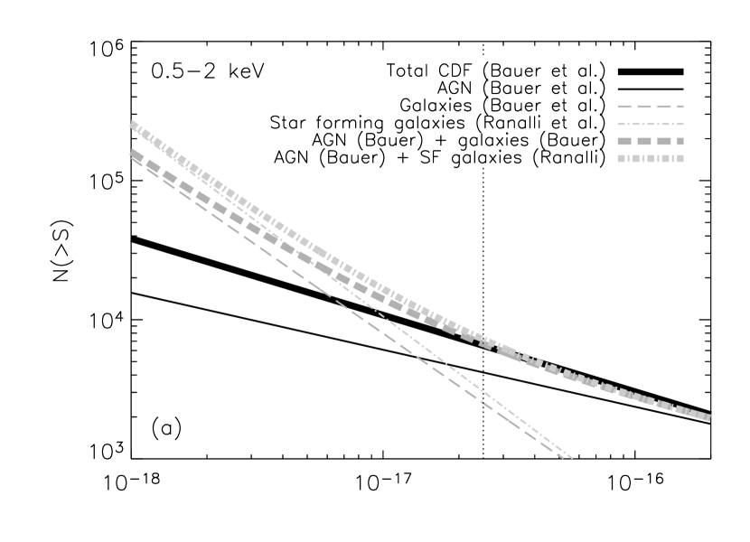
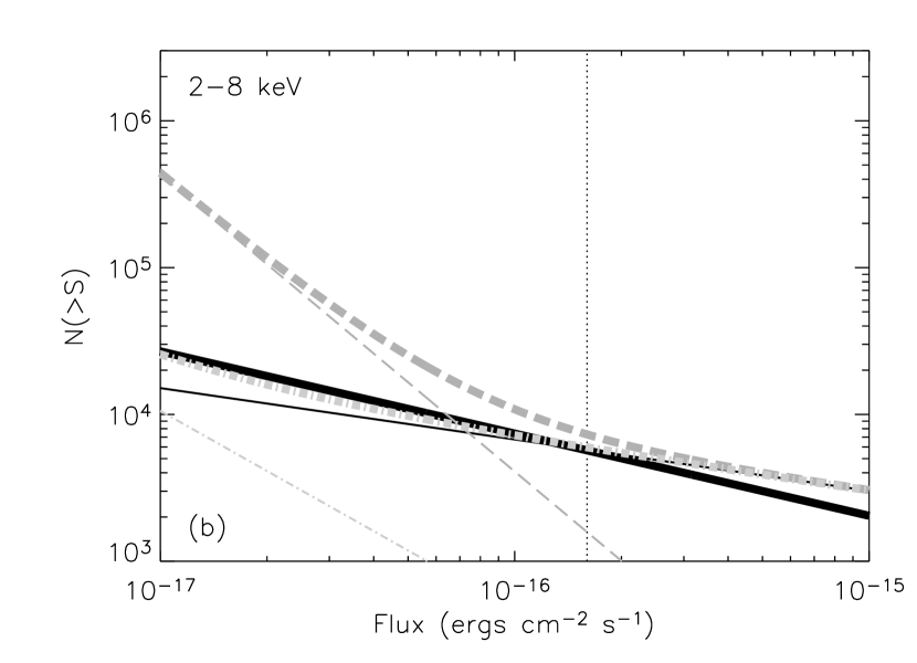
Figure 16.— Best-fit $\log{N}/\log{S}$ distributions for faint sources, for 0.5–2 (top) and 2–8 keV (bottom). The distribution for all CDF detected sources, as well as AGNs and galaxies individually, are taken from B04. An estimate for star-forming galaxies is from R03. The sums of the B04 AGNs and the separate galaxy distributions are also shown. Vertical dotted lines show the A03 CDF-N flux limits.

8.3.4 Galaxy groups?

Finally, we compare our 1–2 keV unresolved signal with surface brightness of galaxy groups, which, according to some estimates (see e.g., Bryan & Voit, 2001, for a high-end prediction), may together contribute at this level to the CXB. For a typical group with average $kT\simeq 2$ keV at $z\simeq 0.1$, the 1–2 keV surface brightness at $r_{200}$, the radius of overdensity 200 times the critical density (i.e., far in its outskirts) would be of order $3\times 10^{-13}$ ergs cm^-2 s^-1 deg^-2(e.g., Vikhlinin et al., 2005). This is 3–4 times below our observed flux. The surface brightness in the core of a group is 2.5–3 orders of magnitude higher. The radius $r_{200}=7-10^{\prime}$ at that redshift; groups closer than that would be big and bright enough to be easily seen in ROSAT surveys, and none is seen near either of the two CDF fields in ROSAT pointed or all-sky data (nor in the Chandra pointings immediately around the CDF-S field). Thus, the diffuse flux is not because either field is in the outskirts of a nearby group. At the same time, more distant galaxy groups at $z\simeq 0.1-0.7$ would be easily detected in these deep Chandra images and excluded by us. Indeed, our excluded extended sources in Fig. 1 are such objects (Giacconi et al., 2002). The surface brightness of still more distant groups and clusters quickly decreases with redshift because of cosmological dimming. For a quantitative estimate of the cumulative brightness of undetected distant groups and clusters One might use the cluster $\log{N}/\log{S}$ (e.g., Rosati et al., 2002) for a quantitative estimate of the cumulative brightness of undetected distant groups and clusters, but it is already obvious that groups cannot contribute significantly to our unresolved 1–2 keV flux.

9. Summary

We measure the absolute intensity of the unresolved cosmic X-ray background, after the exclusion of the sources detected in the deepest Chandra observations, the Chandra Deep Fields North and South. We find significant residual CXB intensity in the 0.5–1 and 1–2 keV bands, and a marginal (2$\sigma$) signal in 2–8 keV band. There is unlikely to be any significant contamination of the signal from ACIS instrumental background.

We find unresolved intensities of $(1.04\pm 0.14)\times 10^{-12}$ ergs cm^-2 s^-1 deg^-2 and $(3.4\pm 1.7)\times 10^{-12}$ ergs cm^-2 s^-1 deg^-2 in the 1–2 and 2–8 keV bands. These values are much higher than the extrapolation of the observed $\log{N}/\log{S}$ curve down to lower fluxes, suggesting an upturn of the distribution below the CDF flux limits, or a truly diffuse component. Combining these results with the total contribution from point sources from CDF and wider-field CXB surveys, we obtain total CXB intensities of $(4.6\pm 0.3)\times 10^{-12}$ and $(1.7\pm 0.2)\times 10^{-11}$ ergs cm^-2 s^-1 deg^-2 for the 1–2 and 2–8 keV bands, respectively. This implies resolved fractions of $77\pm 3$% in 1–2 keV and $80\pm 8$% in 2–8 keV, lower than some previous claims.

References

- Abazajian et al. (2001) Abazajian, K., Fuller, G. M., & Tucker, W. H. 2001, ApJ, 562, 593
- Alexander et al. (2003) Alexander, D. M. et al. 2003, AJ, 126, 539 (A03)
- Barger et al. (2003) Barger, A. J. et al. 2003, AJ, 126, 632
- Basilakos et al. (2005) Basilakos, S., Plionis, M., Georgakakis, A., & Georgantopoulos, I. 2005, MNRAS, 356, 183
- Bauer et al. (2002) Bauer, F. E. et al. 2002, AJ, 123, 1163
- Bauer et al. (2004) Bauer, F. E., Alexander, D. M., Brandt, W. N., Schneider, D. P., Treister, E., Hornschemeier, A. E., & Garmire, G. P. 2004, AJ, 128, 2048 (B04)
- Biller et al. (2002) Biller, B., Plucinsky, P., & Edgar, R. 2002, in Chandra calibration memo, http://cxc.harvard.edu/cal/Acis/Cal_prods/bkgrnd/current/
- Brandt et al. (2001a) Brandt, W. N. et al. 2001a, AJ, 122, 2810
- Brandt & Hasinger (2005) Brandt, W. N. & Hasinger, G. 2005, ARA&A, 43, 827
- Brandt et al. (2001b) Brandt, W. N. et al. 2001b, AJ, 122, 1
- Bryan & Voit (2001) Bryan, G. L. & Voit, G. M. 2001, ApJ, 556, 590
- Cen & Ostriker (1999) Cen, R., & Ostriker, J. P. 1999, ApJ, 514, 1
- Chen et al. (1997) Chen, L.-W., Fabian, A. C., & Gendreau, K. C. 1997, MNRAS, 285, 449
- Cravens (2000) Cravens, T. E. 2000, ApJ, 532, L153
- Davé et al. (2001) Davé, R., et al. 2001, ApJ, 552, 473
- De Luca & Molendi (2004) De Luca, A. & Molendi, S. 2004, A&A, 419, 837 (DM04)
- della Ceca et al. (1999) della Ceca, R., Castelli, G., Braito, V., Cagnoni, I., & Maccacaro, T. 1999, ApJ, 524, 674
- Dickey & Lockman (1990) Dickey, J. M. & Lockman, F. J. 1990, ARA&A, 28, 215
- Garmire et al. (1992) Garmire, G. P., Nousek, J. A., Apparao, K. M. V., Burrows, D. N., Fink, R. L., & Kraft, R. P. 1992, ApJ, 399, 694
- Gendreau et al. (1995) Gendreau, K. C. et al. 1995, PASJ, 47, L5