SNSPH: A Parallel 3-D Smoothed Particle Radiation Hydrodynamics Code

Abstract

We provide a description of the SNSPH code—a parallel 3-dimensional radiation hydrodynamics code implementing treecode gravity, smooth particle hydrodynamics, and flux-limited diffusion transport schemes. We provide descriptions of the physics and parallelization techniques for this code. We present performance results on a suite of code tests (both standard and new), showing the versatility of such a code, but focusing on what we believe are important aspects of modeling core-collapse supernovae.

1 Introduction

SNSPH is a particle-based code, using smooth particle hydrodynamics (SPH) to model the Euler equations and a flux-limited diffusion package to model radiation transport. Its tree algorithm is designed for fast traversal on parallel systems (Warren & Salmon 1993,1995) and has been shown to scale well up to high processor number on a wide variety of computer architectures. The increased synchronization required for the transport algorithm limits this scalability to roughly 512 processors on current parallel computers for the 1-10 million particle core-collapse calculations that are feasible with our current codes and current computing power.

SNSPH has now been used in several papers appearing in the literature studying a range of problems from stellar collapse (Fryer & Warren 2002,2004; Fryer 2004; Fryer & Kusenko 2005) to supernova explosions and supernova remnants (Hungerford et al. 2003, 2005; Young et al. 2005; Rockefeller et al. 2005a; Fryer et al. 2005) to models of massive binaries and winds from these binaries (Fryer & Heger 2005; Fryer, Rockefeller, & Young 2005) to models of both the gas and disk evolution in the Galactic Center (Rockefeller et al. 2004, 2005b, 2005c). But none of these papers has provided a detailed description of the SNSPH code itself. Here we describe these details: §2 describes much of the physics implementation from gravity to hydrodynamics to radiation transport; and §3 describes many of the numerical techniques used in this particle-based code, focusing on many of the computational techniques required to make such a scheme scalable. In §4, we show the results of SNSPH for a number of tests (both standard and new) used to confirm the validity of SNSPH for core-collapse simulations. Astrophysics problems tend to be too complex for most standard code tests to completely confirm the validity of the code for that specific astrophysics problem. We present a small suite of tests to show the broad range of physics that must be tested to model core-collapse. These tests demonstrate the wide applicability of this SNSPH code, but further testing is required to truly test all the physics in the code. We conclude with a list of strengths and weaknesses of SNSPH.

2 Physics Implementation

As with many astrophysics problems, solving the supernova problem requires a wide range of physics. This physics must be, in one way or another, implemented into the numerical code simulating this phenomena. In this section, we describe the major aspects of the physics incorporated into SNSPH: gravity, hydrodynamics (including the equation of state), and radiation transport (including opacities). Where possible, we have sought to make the code modular to facilitate modifications in the different microphysics packages from the equation of state to neutrino cross-sections and emission routines.

2.1 Gravity

Newton’s second law of motion and law of gravitation provide an expression for the acceleration of one body under the combined gravitational influence of a set of $N-1$ other bodies, according to

$$\frac{d^{2}\vec{x}_{i}}{{dt}^{2}}=\sum_{j\neq i}^{N}\vec{a}_{ij}=\sum_{j\neq i}^{N}\frac{Gm_{j}\vec{r}_{ij}}{{|\vec{r}_{ij}|}^{3}},$$ (1)

where $\vec{r}_{ij}\equiv\vec{x}_{i}-\vec{x}_{j}$. Using this equation to calculate the acceleration for one body requires $N-1$ evaluations of the term inside the sum, so determining the accelerations of all $N$ bodies in a simulation requires $N(N-1)$ or $O(N^{2})$ operations. Performing this type of pairwise summation to calculate gravitational interactions is prohibitively expensive for all but the smallest sets of bodies, even on the fastest supercomputers.

A number of approximate methods have been developed to calculate gravitational forces among large numbers of bodies by considering as one interaction the total effect of a set of bodies on one body, or the effect of one set of bodies on another set, with time requirements that scale as $O(N\log N)$ or $O(N)$, respectively. Codes that use adaptive tree structures to subdivide the volume of a simulation and distinguish between nearby and distant bodies can easily implement such accelerated techniques; our code uses such a tree and is therefore one of a class of codes called “treecodes”. This class includes many SPH codes such as Gadget Springel et al. (2001) and Gasoline Wadsley et al. (2004) as well as particle mesh codes Suryadeep (2004) and some Adaptive Mesh Refinement Codes such as RAGE Coker, R. et al. (2005).

Knowledge of the spatial arrangement of bodies in a simulation allows the treecode to distinguish between “nearby” bodies, for which direct pairwise calculation of gravitational forces is appropriate, and “distant” bodies, for which an approximate technique will yield a sufficiently accurate value for the force. The simplest approximation combines a set of distant bodies into one object with a total mass equal to the sum of the masses of the individual bodies in the group, positioned at the location of the center of mass of the group:

$$\sum_{j\neq i}-\frac{Gm_{j}\vec{r}_{ij}}{{|\vec{r}_{ij}|}^{3}}\approx-\frac{GM\vec{r}_{i,cm}}{{|\vec{r}_{i,cm}|}^{3}},$$ (2)

where $\vec{r}_{i,cm}=\vec{r}_{i}-\vec{r}_{cm}$, $\vec{r}_{cm}$ is the location of the center of mass of the group of bodies, and $M$ is the total mass of the group. In principle this equation could include additional terms on the right-hand side to account for the quadrupole and higher moments of the mass distribution. In practice, equivalent accuracy and higher performance is obtained for moderate levels of accuracy ($\sim$ 0.1 percent) by including only the monopole contribution (and, implicitly, the dipole contribution, which is equal to zero) and using an appropriate criterion for determining when the approximation is accurate enough.

Some criterion must be used to determined when the multipole approximation in equation 2 is sufficiently accurate to use instead of direct summation of the accelerations due to each body in the set. This criterion is called the “multipole acceptability criterion” or MAC. Many different MACs have been proposed, and several are in widespread use. Salmon & Warren (1994) analyzed the worst-case behavior of several different MACs and developed a technique to determine a strict upper limit on the errors in each acceleration calculation. As described in (Warren & Salmon 1993,1995), we use a MAC that incorporates such an error estimate into the calculation of a critical radius, according to

$$r_{c}\geq\frac{b_{max}}{2}+\sqrt{\frac{{b_{max}}^{2}}{4}+\sqrt{\frac{3B_{2}}{\Delta_{interaction}}}},$$ (3)

where $b_{max}$ is the size of the cell and $B_{2}=\sum_{i}m_{i}{|\vec{r}_{i}-\vec{r}_{cm}|}^{2}$ is the trace of the quadrupole moment tensor. A body and cell separated by a distance greater than $r_{c}$ can use equation 2 to evaluate the acceleration, and the absolute error is guaranteed to be less than $\Delta_{interaction}$; a body and cell closer than $r_{c}$ must use pairwise summation for each body in the cell, or subdivide the cell into smaller cells and reconsider the interactions, to ensure that the error is not larger than that tolerance.

2.2 SPH Hydrodynamics

The particle-based structure of our code allows us to easily implement the smooth particle hydrodynamics (SPH) to model the Euler (inviscid) equations. SPH, invented in 1977 (Lucy 1977, Gingold & Monaghan 1977), has become the primary multi-dimensional Lagrangian technique used in astrophysics. Its versatility allows it to be used on a variety of astrophysics problems (see Benz 1988; Monaghan 1992 for a review). Many variants of SPH have been developed and a number of excellent reviews on the SPH technique, and its variations, already exist (Benz 1989; Monaghan 1992; Morris 1996; Rasio 1999; Monaghan 2005); we provide a brief review here and direct readers interested in more details to the above reviews. Our code was developed using the Benz version of SPH (Benz 1984, 1988, 1989) as a model and is nearly identical to those codes based on this version of SPH.

2.2.1 Brief SPH Primer

SPH is a particle based method where particles act as interpolation points to determine matter conditions throughout the simulation space. Consider the following integral representation of the quantity $A$:

$$A_{s}(\vec{r})=\int A(\vec{r}^{\prime})W(\vec{r}-\vec{r}^{\prime},h)dr^{\prime}$$ (4)

where $W(\vec{r}-\vec{r}^{\prime},h)$ (the “kernel”) has the following properties:

$$\int W(\vec{r}-\vec{r}^{\prime},h)dr^{\prime}=1$$ (5)

and

$$\lim_{h\to 0}W(\vec{r}-\vec{r}^{\prime},h)=\delta(\vec{r}-\vec{r}^{\prime}).$$ (6)

By integrating $A$ with our kernel, $A_{s}$ is the “smoothed” version of $A$ (hence the origin of the “Smooth” in SPH). Note that $A_{s}$ approaches $A$ as $h\to 0$. If we expand $A(\vec{r})$ in a Taylor series, we find that:

$$A_{s}(r)=A(r)+c(\nabla^{2}A)h^{2}+O(h^{3})$$ (7)

This SPH formulism introduces an error of order $h^{2}$ in the estimate of the quantity $A(r)$. Discretizing this method, the integral over $A$ is reduced to a summation over a number of points (particles) in space:

$$A_{s}(r)=\sum_{j}A_{j}(m_{j}/\rho_{j})W(\vec{r}-\vec{r}_{j},h)$$ (8)

where $A_{j}$, $m_{j}$, and $\rho_{j}$ are the respective values of $A$, the mass, and the density of particle $j$. The structure of the smoothing is determined by the kernel $W(\vec{r}-\vec{r}^{\prime},h)$ where $h$ denotes the size over which the smoothing occurs (see below).

Although any kernel will work as long as it satisfies equations 5 and 6, determining the best kernel for a given problem can be a black art. One of the simplest kernels, and the one we use for most of our calculations (although we also use other spline kernels) is a cubic spline kernel:

$$W(r,h)=\pi^{-1}h^{-3}\begin{cases}1-1.5v^{2}+0.75v^{3}&\text{if $0\leq v\leq 1$,}\cr 0.25(2-v)^{3}&\text{if $1\leq v\leq 2$,}\cr 0.&\text{otherwise,}\end{cases}$$

where $v=r/h$. With this kernel, a given interpolation point (particle) contributes to the value of $A(r)$ only if $r$ is within $2h$ of that particle. The value of $h$ for a given particle $i$, termed the “smoothing length”, is allowed to vary with time using the relation presented in Benz (1989):

$$dh_{i}/dt=-1/3(h_{i}/\rho_{i})(d\rho_{i}/dt)$$ (9)

This variation is necessary to ensure full spatial coverage by the particles (we would like any position to overlap with a base number of particles) and, as long as $h$ varies on a scale similar to other variables, the errors remain of $O(h^{2})$ (Hernquist & Katz 1989). We define the interaction between a particle $i$ and a neighboring particle $j$ by evaluating a mean value $h\equiv(h_{i}+h_{j})/2$. We additionally set limits for the number of neighbors (the standard range for our 3-dimensional models is between $\sim$40 and $\sim$80 neighbors). In the extreme case that the number of neighbors falls above (or below) these maximum (minimum) values, we additionally lower (raise) $h_{i}$ by a configurable amount on each timestep (typically a factor of 0.002-0.1) to enforce this range of neighbors (this occurs rarely, if at all, for a given particle during the course of a simulation).

We can now use our interpolation points to calculate the value of any quantity and its derivatives over our spatial domain. The density at position $i$ is simply:

$$\rho_{i}=\sum_{j}m_{j}W(\vec{r}_{i}-\vec{r}_{j},h).$$ (10)

As with any numerical technique, there is more than one way to discretize our system. This is most apparent in the calculation of derivatives. For example, in principal, the gradient of a function $A$ at particle $i$ is just:

$$\nabla A_{i}=\sum_{b}A_{j}(m_{j}/\rho_{j})\nabla W(\vec{r}_{i}-\vec{r}_{j},h).$$ (11)

In practice, it is more accurate to use,

$$\nabla A_{i} = 1/\rho[\nabla(\rho A)-A\nabla\rho]$$ (12)

$$= 1/\rho_{i}\sum_{j}(A_{j}-A_{i})m_{j}\nabla W(\vec{r}_{i}-\vec{r}_{j},h).$$ (13)

The Morris (1996) review includes quite a bit of discussion about these “techniques” used to improve SPH, also noting the situations when one technique might be better than another. We follow the Benz version of SPH for all our discretization assumptions in solving the hydrodynamics equations.

2.2.2 Continuity Equation

The Benz version of SPH is a true Lagrangian code - the mass and number of particles is conserved, so the total mass in the system is also conserved.

2.2.3 Momentum Equation

We evaluate momentum and energy conservation for the particles themselves and assume an inviscid gas. Hence, the hydrodynamic equations reduce to the Lagrangian form of the Euler equations:

$$d\vec{v}_{i}/dt=-1/\rho_{i}(\nabla P)_{i}$$ (14)

where $\vec{v}_{i}=d\vec{r}_{i}/dt$ and $P_{i}$ is the pressure of particle $i$. If we simply use equation 12, the pressure gradient for particle $i$ is written:

$$(\nabla P)_{i}=1/\rho_{i}\sum_{j}m_{j}(P_{j}-P_{i})\nabla_{i}W_{ij}$$ (15)

where $W_{ij}=W(\vec{r}_{i}-\vec{r}_{j},h)$. Although such a scheme can be used, it is not symmetric (and hence does not conserve linear and angular momentum). We can instead write:

$$\nabla P/\rho=\nabla(P/\rho)+P/\rho^{2}\nabla\rho$$ (16)

Now using equation 12 on this representation, we get:

$$d\vec{v}_{i}/dt=-\sum_{j}m_{j}(P_{i}/\rho_{i}^{2}+P_{j}/\rho_{j}^{2})\nabla_{i}W_{ij}.$$ (17)

Let’s confirm that this algorithm conserves linear momentum. The force on particle $i$ due to particle $j$ is equal to the negative force on particle $j$ due to particle $i$:

$$m_{i}d\vec{v}_{i}/dt=m_{i}m_{j}(P_{i}/\rho_{i}^{2}+P_{j}/\rho_{j}^{2})\nabla_{i}W_{ij}=-m_{j}d\vec{v}_{j}/dt,$$ (18)

where we have taken advantage of the fact that the kernels are anti-symmetric $\overrightarrow{\nabla}_{i}W_{i}(|\overrightarrow{r}_{i}-\overrightarrow{r}_{j})|,h)=-\overrightarrow{\nabla}_{j}W_{j}(|\overrightarrow{r}_{i}-\overrightarrow{r}_{j})|,h)$. We will show that angular momentum is conserved in section 4.

2.2.4 Energy Conservation

Most hydrodynamics codes evolve either the total energy (kinetic + internal) or the internal (thermal) energy alone. In a system with gravity, the total energy also can include the gravitational potential energy. Evolving the total energy ensures a better conservation of the total energy. But in astrophysics, accurate temperatures (and hence energies) are important even in cases where the gravitational potential and kinetic energies dominate the total energy by many orders of magnitude. To obtain reliable internal energies, it is often better to evolve the internal energy alone in the energy equation. The evolution of the specific internal energy $u$ is

$$du/dt=-(P/\rho)\nabla\cdot\vec{v},$$ (19)

corresponding to the following SPH formulation:

$$du_{i}/dt=P_{i}/\rho_{i}^{2}\sum_{j}m_{j}(\vec{v}_{i}-\vec{v}_{j})\cdot\nabla_{i}W_{ij}$$ (20)

See Morris (1996) for other valid SPH formulations of the energy equation.

It is easy to show that this formulation combined with our momentum equation conserves total energy (kinetic and thermal energies). The total energy for all particles is given by:

$$d/dt\sum_{i}m_{i}u_{i}=\sum_{i}\sum_{j}m_{i}m_{j}P_{i}/\rho_{i}^{2}(\vec{v}_{i}-\vec{v}_{j})\cdot\nabla_{i}W_{ij}$$ (21)

By interchanging indices and again making use of the identity $\nabla_{i}W_{ij}=-\nabla_{j}W_{ij}$, we get

$$d/dt\sum_{i}m_{i}u_{i}=\sum_{i}\sum_{j}m_{i}m_{j}(P_{i}/\rho_{i}^{2}+P_{j}/\rho_{j}^{2})(\vec{v}_{i}-\vec{v}_{j})\cdot\nabla_{i}W_{ij}.$$ (22)

Comparing this to equation 17, we find:

$$d/dt\sum_{i}m_{i}u_{i}=d/dt(1/2\sum_{i}m_{i}v_{i}^{2})$$ (23)

which shows that the work done by pressure forces changing the kinetic energy comes at the expense of the internal energy, ensuring the conservation of total energy.

In core-collapse, it is often better to follow the entropy, instead of the internal energy, of matter. For degenerate matter, the temperature can vary wildly over small changes of the internal energy. Entropy varies more rapidly with temperature in degenerate conditions. By using entropy as the energy parameter, we get more stable temperature values. We use the same hydrodynamics equations, setting $ds_{i}/dt=(1/T)(du_{i}/dt)$ where $T$ is the matter temperature.

2.2.5 Artificial Viscosity

We have limited our description of hydrodynamics to inviscid (Euler) equations. It is well known that any Euler method with finite resolution is unable to describe shocks and will result in large, unphysical, oscillations unless one includes some sort of viscosity, low order diffusion or a Riemann solver. Although Godunov-type methods have been developed for SPH (Inutsuka 1994; Monaghan 1997; Inutsuka 2002), most techniques introduce a viscosity term to handle shocks (Benz 1989; Monaghan 1992, Monaghan 2005):

$$\Pi_{ij}=\begin{cases}(-\alpha\bar{c}\mu_{ij}+\beta\mu_{ij}^{2})/\bar{\rho}_{ij}&\text{if $(\vec{v}_{i}-\vec{v}_{j})\cdot(\vec{r}_{i}-\vec{r}_{j})\leq 0$,}\cr 0&\text{otherwise,}\end{cases}$$

where

$$\mu_{ij}=\frac{h(\vec{v}_{i}-\vec{v}_{j})\cdot(\vec{r}_{i}-\vec{r}_{j})}{|\vec{r}_{i}-\vec{r}_{j}|^{2}+\epsilon h^{2}},$$ (24)

$\bar{\rho}_{ij}=1/2(\rho_{i}+\rho_{j})$ and $\bar{c}_{ij}=1/2(c_{i}+c_{j})$ are the average of the densities and sound speeds of the interacting particles, $\alpha$ and $\beta$ are the bulk and von Neumann-Richtmyer viscosity coefficients respectively (typically set to 1.5 and 3.0), and $\epsilon$ is a factor to avoid divergences at small separations (typically set to 0.01).

The momentum and energy (internal + kinetic) equations can now be rewritten to include this viscosity:

$$d\vec{v}_{i}/dt=-\sum_{j}m_{j}(P_{i}/\rho_{i}^{2}+P_{j}/\rho_{j}^{2}+\Pi_{ij})\nabla_{i}W_{ij}$$ (25)

and

$$du_{i}/dt=P_{i}/\rho_{i}^{2}\sum_{j}m_{j}(\vec{v}_{i}-\vec{v}_{j})\cdot\nabla_{i}W_{ij}+1/2\sum_{j}m_{j}\Pi_{ij}(\vec{v}_{i}-\vec{v}_{j})\cdot\nabla_{i}W_{ij}.$$ (26)

Clearly, the addition of the artificial viscosity term retains our total (kinetic + internal) energy conservation.

2.2.6 Equation of State

To complete these equations, we must include an equation of state to determine pressures from internal energies or entropies. Our basic SPH scheme includes equations of state for isothermal and ideal gases. But we have also included a number of equations of state and the code has thusfar not encountered any problems incorporating new equations of state.

The most complex equation of state we have in the code is the one we have used in most of our supernova simulations. For the core-collapse problem we use an equation of state combining the nuclear equation of state by Lattimer & Swesty (1991) at high densities and the Blinnikov et al. (1996) equation of state at low densities. Nuclear burning is approximated by a nuclear statistical equilibrium scheme (Hix & Thielemann 1996).

The Lattimer & Swesty (1991) equation of state can be used from densities below $10^{9}{\rm g\,cm^{-3}}$ up to densities above $10^{15}{\rm g\,cm^{-3}}$. However, an error in the energy levels of this equation of state cause it to give incorrect answers below $10^{11}{\rm g\,cm^{-3}}$ (Timmes et al. 2005) and be aware that we do not know the true behavior of matter above nuclear densities and we expect this part of the equation of state to change with time. It is valid for electron fractions from 0.03 up to 0.5. If the electron fraction exceeds this value, we assume the pressure is set to 0.5. In typical simulations, we use the Lattimer & Swesty equation of state for matter above $10^{11}{\rm g\,cm^{-3}}$. Below $10^{11}{\rm g\,cm^{-3}}$, we use the Blinnikov equation of state. This equation of state is valid to densities as low as $100{\rm g\,cm^{-3}}$. Below these densities, the equation of state is comparable to an ideal gas equation of state.

The nuclear statistical equilibrium scheme is used for material in the Blinnikov equation of state with temperatures above $5\times 10^{9}$K (depending upon the problem, this value is sometimes set a factor of 2 lower or higher). This scheme uses 16 species, focusing on the iron-peak elements from ${}^{54}Fe$ to ⁸⁶Kr with typical Q-values for reactions among stable nuclei heavier than silicon lying between 8-12MeV. The version of the equation of state we describe here is not tabular, but a set of analytic function calls. Timmes et al. (2006) have developed a tabular version of this equation of state which is currently being tested.

We have added small networks, such as the 14-element alpha network by Benz, Thielemann, & Hills (1989) to the code to follow the burning in the non-steady state. In general, the burning time-step is much shorter than the hydrodynamic timestep, so the burning is done in a sub-cycle using Newton-Raphson iterations to converge. For most core-collapse calculations where we include this network, burning is only considered for temperatures above $8\times 10^{7}$K and the network is switched over to nuclear statistical equilibrium at $5\times 10^{9}$K. Comparisons with large networks have shown that this network does not produce accurate yields, but the energies are reasonable (Young et al. 2005).

We have also added an equation of state to model the basalt and iron material in planetary cores (Tillotson 1962). The addition of new equations of state is a straightforward exercise ($<1$ day of work).

2.3 Radiation Transport

The radiation transport scheme currently implemented in the SPH code is based on the 2-dimensional explicit, flux-limited transport scheme developed by Herant et al. (1994). Flux-limited diffusion is a moment closure technique where the equations are closed in the first moment. For neutrino diffusion, we transport the neutrino number and the advection term in the flux limited diffusion equation is simply:

$$1/c\partial n_{\nu}/\partial t=\Lambda\nabla n_{\nu},$$ (27)

where $n_{\nu}$ is the neutrino number, c is the speed of the neutrinos (set to the speed of light) and $\Lambda$ is the flux-limiter. Here we describe the 3-dimensional adaptation of this scheme. We also comment on a number of peculiarities of this scheme that should be understood before its use.

In the current version of the code, we consider the transport of 3 neutrino species ($l=\nu_{e},\bar{\nu_{e}},\nu_{x}$ where $\nu_{x}$ corresponds to the $\tau,\mu$ neutrinos and their anti-particles that are all treated equally). Because neutrino number is the conserved quantity, we transport neutrino number and then determine the energy transport by using the mean neutrino energies. The radiation transport scheme in our SPH code is modeled after the technique to calculate forces in SPH: we calculate symmetric interactions between all neighbor particles. Hence, our flux-limited diffusion scheme calculates the radiation diffusion in or out of a particle by summing the transport over all neighbors (the equivalent of all bordering cells in a grid calculation). The neutrino transport for particle i is given by:

$$dn^{i}_{\nu_{l}}/dt=\sum_{j}\Lambda^{ij}_{\nu_{l}}(n^{j}_{\nu_{l}}b^{j\rightarrow i}_{\nu_{l}}-n^{i}_{\nu_{l}}b^{i\rightarrow j}_{\nu_{l}})\nabla W^{ij}m^{j}/\rho^{j}$$ (28)

and the corresponding energy transport is:

$$de^{i}_{\nu_{l}}/dt=\sum_{j}\Lambda^{ij}_{\nu_{l}}(\epsilon^{j}_{\nu_{l}}n^{j}_{\nu_{l}}b^{j\rightarrow i}_{\nu_{l}}-\xi^{i\rightarrow j}\epsilon^{i}_{\nu_{l}}n^{i}_{\nu_{l}}b^{i\rightarrow j}_{\nu_{l}})\nabla W^{ij}m^{j}/\rho^{j}$$ (29)

where $n^{i}_{\nu_{l}},e^{i}_{\nu_{l}}$ are, respectively, the neutrino density and energy density in particle i for species $\nu_{l}$, $\epsilon_{\nu_{l}}^{i}$ is the mean neutrino energy (an average energy taking into account the $\epsilon_{\nu_{l}}^{2}$ dependence of the neutrino opacity), and $\xi^{j\rightarrow i}$ is the redshift correction for $\epsilon_{\nu_{l}}^{j}$ as seen by particle i. $b^{i\rightarrow j}_{\nu_{l}}$ are the fermion blocking factors for neutrinos.

$\Lambda^{ij}_{\nu_{l}}$ is effectively the limiter for the flux-limited transport scheme (we have modified the definition slightly to fit in our numerical equations). The simplest such scheme for 3-dimensions is:

$$\Lambda^{ij}_{\nu_{l}}=min(c,D^{ij}_{\nu_{l}}/r^{ij})$$ (30)

where $c$ is the speed of light, $D^{ij}_{\nu_{l}}=2D^{i}_{\nu_{l}}D^{j}_{\nu_{l}}/(D^{i}_{\nu_{l}}+D^{j}_{\nu_{l}})$ is the harmonic mean of the diffusion coefficients for the species $\nu_{l}$ of particles i and j and $r^{ij}$ is the distance between particles i and j. This limiter was used by Herant et al. (1994) and, for comparison with Herant et al. (1994), by Fryer & Warren (2002), but we have used a number of other flux-limiters, all of which are valid under this transport scheme (Fryer et al. 1999). The opacities used to determine the diffusion coefficients are given in Herant et al. (1994).

Beyond some radius in a core-collapse simulation, neutrinos are essentially in the free-streaming regime where transport is not necessary (unless one wants to truly follow the radiation wave as it progresses through the star). We do not model transport beyond this “trapping” radius. Instead we sum up all neutrinos that transport beyond this radius and emit them using a light-bulb approximation. That is, the material beyond this radius sees a constant flux and we can determine the amount of energy a particle gains ($dE_{i}/dt$) from neutrino interactions simply by using the free-streaming limit:

$$dE_{i}/dt=L_{\nu}\left(1.0-e^{-\Delta\tau_{i}}\right)$$ (31)

where $L_{\nu}$ is the neutrino luminosity and $\Delta\tau_{i}$ is the optical depth of a particle $i$. This assumption is only valid if the total amount of energy imparted ($\sum_{i}dE_{i}/dt$) from the neutrinos onto the matter is much less than the total neutrino flux ($L_{\nu}$). To guarantee this, we determine this trapping radius by evolving it with time such that $(\sum_{i}dE_{i}/dt)/L_{\nu}$ is always less than some value. This value was originally set to 0.1 by Herant et al. (1994), but in recent calculations, we use 0.05.

Such a scheme can be easily converted into multi-group, but such modifications have not yet been done. The scheme scales reasonably well on multiple processors (for a 5 million particle run, the code has scaled nearly linearly up to 256 processors on the Space Simulator Beowulf cluster and up to 512 processors on the ASC Q machine at Los Alamos National Laboratory). In part, this scalability is due to the explicit nature of the transport scheme. In general, explicit transport schemes strongly limits timesteps as the speed of light, not sound, constrains the duration of the timestep. In core-collapse supernovae, this constraint is not too onerous because the sound speed is nearly a third the speed of light anyway, so the explicit transport scheme leads to only a factor of 3 decrease in the timestep. But this explicit flux-limited transport scheme can be used in a much wider variety of problems where the mean free path is very short for the smallest particles. Such scenarios occur in many astrophysics problems.

Before we show how well SNSPH performs on our suite of test problems, let’s describe the computational techniques used to make this code run efficiently on parallel architectures.

3 Computational Issues

On a single processor, careful attention to the computational details can significantly accelerate a code’s performance. For large-scale parallel architectures, these details are critical to taking full advantage of these supercomputers. Unfortunately, the more complex the code becomes, the more ingenuous the computational techniques must be to preserve scalability. Here we discuss just the basic computational issues, focusing on our tree algorithm (see also Warren & Salmon 1993, 1995) and the basic parallelization issues arising from use of this tree. We conclude with a discussion of the timestep integrator.

3.1 Treecode

The calculation of gravitational forces between bodies in a N-body simulation and the identification of neighbors in a SPH calculation are both accelerated significantly through the use of a treecode, in which a hierarchical “tree” data structure is constructed to represent the spatial arrangement of bodies in a simulation. Our code uses a “parallel hashed oct-tree algorithm” (Warren & Salmon 1993, 1995), in which each node in the tree can have up to eight “daughter” nodes below it. The “root” of the tree (often imagined to be at the top of the tree in computer science discussions) represents the entire volume of a simulation; each of the root’s eight daughter nodes represents one octant of that overall volume. A complete hierarchical representation of the volume can be created by recursively subdividing each octant and adding more levels of daughter nodes to the tree until some stopping condition is reached. In our implementation of a treecode, we stop subdividing a volume when that volume contains zero particles or only one particle; the node representing that volume in the tree is called a “leaf” node and has no daughters of its own. By performing traversals of the hierarchical tree structure, the treecode can rapidly distinguish between nearby and distant particles and accelerate the calculation of gravitational and pressure forces in simulations.

In descriptions of N-body techniques, the term “body” generally refers to one of the fundamental entities being simulated. In smoothed particle hydrodynamics, the interacting entities are logically called “particles”. In the following discussion, the terms “particle” and “body” are used interchangeably; both refer to a data-carrying entity in a simulation. The term “cell” refers to a cubical region of space containing (possibly zero) particles; a cell is represented as a node in the tree data structure that stores data used by the treecode, and phrases like “daughter cell” refer to the combined knowledge about a spatial region in the simulation and its topological location within the tree.

Conventional implementations of tree structures represent connections between nodes within the tree as pointers stored in parent nodes that point to the memory locations of the daughters. This technique is difficult to implement on a parallel machine: a parent node on one processor may have daughter nodes located on different processors. Our treecode instead uses multi-bit “keys” to identify particles and cells in the tree; a hash table translates keys into actual memory locations where cell data is stored (hence the word “hashed” in the phrase “parallel hashed oct-tree algorithm”). This level of indirection enables uniform handling of local and non-local cell data; the algorithm that maps hash keys to cell data can request non-local data from other processors and only make it available to the local process once it has arrived.

3.1.1 Key Construction

As was mentioned above, each body and cell in the tree is identified by a key; by using the key as an index into a hash table, the code can quickly locate or request delivery of data about any entity in a simulation, and the hash algorithm transparently handles retrieval of data stored on other processors in a parallel machine. The algorithm described below generates keys that, when sorted, arrange the particles into Morton order within the volume of solution; such keys are often called “Morton keys”. Morton ordering results in a list of particles that fairly well reflects spatial locality of bodies in the tree, i.e. particles with Morton keys that fall near each other in the sorted list of keys generally lie near each other in the simulated volume. However, particles sorted into e.g. Peano-Hilbert order can exhibit an even higher correlation between proximity in the sorted key list and proximity in space, which can lead to more efficient distribution of data on a parallel computer, so modern treecodes have tended to use Peano-Hilbert keys to refer to particles (see, e.g., Springel 2005). Our treecode supports both Morton and Peano-Hilbert keys, but in practice we have found no noticeable difference in performance; we generally use Morton keys, as described below.

Each Morton key is a set of $l_{k}$ bits derived from the $d$ floating point coordinates of a body in $d$-dimensional space. One bit is reserved as a placeholder, for reasons explained below, which leaves $n=(l_{k}-1)/d$ bits to represent each of the coordinates of a body. To generate a key for each particle in a simulation, we start by calculating the spatial extent of the simulation and then divide the largest spatial dimension into $2^{n}$ equal intervals; the intervals can then be indexed by a $n$-bit integer. For simplicity, the same interval spacing is used for the other (smaller) spatial dimensions as well. Each floating point coordinate of each body in the simulation is mapped to the $n$-bit integer index of the spatial interval containing that coordinate.

To construct a key from the $d$ integers derived from the spatial coordinates of a body, the integers are interleaved bit-by-bit. The result is a key composed of $n$ groups of bits, each of length $d$, where the bits in the $i$th group are the $i$th bits of each of the integers identifying the body, arranged in dimension order.

3.1.2 Hashing

The mapping between keys and pointers to cell data is maintained via a hash table. The actual hashing function is very simple—we select the $h$ least-significant bits of the key—but because a key reflects the spatial location of the associated cell, the spatial distribution of bodies and cells determines which hash table entries are filled. Each hash table entry is stored in a “hcell”; the hcell contains a pointer to the actual cell data (if the data is local) and maintains knowledge of the state of the cell data—whether it is local or nonlocal, or if it has been requested from another processor.

3.1.3 Tree Construction

The key length $l_{k}$ determines how many levels of cells the tree can represent, or how close two particles can be, relative to the spatial extent of the simulation, and still be stored separately in the tree. Intermediate (i.e. non-leaf) cells in the tree can be represented in the same key space as individual bodies if the highest bit of every key is set to 1 as a placeholder; the position of this placeholder (the highest non-zero bit) in a cell’s key indicates the depth of that cell in the tree. Given a key for any cell or body, the key of the parent cell can be found by right-shifting the key by $d$ bits (i.e. the number of spatial dimensions). The root of the tree has a key of “1”—the placeholder bit is the lowest (and only) bit in the key.

Keys constructed for bodies are used first to sort the particles and distribute them across the set of processors used in a parallel calculation (see §3.2). After each processor receives the bodies assigned to it, a tree of cells is constructed and all local bodies are inserted into the tree. The key associated with a body is not changed when the body is added to the tree; instead, the body is associated with a cell, and the cell key represents the location and depth of the cell in the tree. The first body is inserted into a cell immediately below the root. Subsequent cells are inserted by starting from the location of the previous cell and searching for the appropriate location in the tree; because the bodies are already sorted, the correct location is usually very close to the previously-inserted cell. Often the insertion of a new cell will require a previously-inserted cell to be split, and both the old and new cell will be moved to a lower location in the tree; empty cells are inserted at each tree level between the old and new locations.

An intermediate cell is “finished” when it is clear that no new bodies will be inserted below it—because the bodies have already been sorted into Morton order, it is easy to determine when no additional bodies will be inserted below a particular cell. The process of “finishing” includes calculating the total mass and spatial extent of the set of all daughter cells, which permits fast evaluation of multipole contributions during calculation of gravitational forces among groups of particles.

3.2 Parallelization

Sorting the list of body keys is equivalent to arranging the bodies in Morton order. Morton ordering does a reasonably good job of maintaining locality of data in the sorted list; bodies that are close together in space end up close to each other in the list. This ordering of bodies also allows easy domain decomposition for parallelization; data can be distributed over a set of processors in a parallel machine by cutting the list of bodies into “equal-work” lengths and sending each list section to a different processor. The “work” required to update a particle is usually defined as the number of interactions in which the particle participated during the previous timestep, which generally results in good load-balancing. It is also possible to adjust the estimated work associated with any set of particles to account for, e.g., complex equation of state calculations which take a predictable number of iterations to converge.

Parallel tree construction adds one additional step to the process described in §3.1; after building a local tree, each processor finds and transmits a set of “branch cells” to all other nodes. The set of branch cells on a given processor is the coarsest set of cells that contains all of the data stored on that processor. Branch cells are the highest “finished” cells in the local tree; all cells and bodies below a branch cell are also stored on the processor, while cells above the branch cell include regions of space containing particles stored on other processors. Every processor broadcasts its branch cells to every other processor, so that each processor can directly request non-local cell data from the correct processor during traversals of the tree.

Characterizing the performance of parallel scientific codes is difficult, and trying to doing so for SNSPH presents all the usual pitfalls. Per-processor performance metrics, and scaling of performance with number of processors in a parallel calculation, both vary strongly depending on the size of simulation under consideration, the hardware platform on which the simulation is run, and even the particular physical or numerical conditions present in the simulation. Scaling for SNSPH is linear on hundreds through thousands of processors on modern supercomputers, as long as the problem being simulated is sufficiently large, and the definition of ”large” for a given computer depends on the details of the CPU architecture, memory subsystem, node interconnects, and other system components. For a core-collapse simulation including all physics modules within SNSPH, a 4-million-particle set of initial conditions is sufficiently large to support nearly linear scaling on up to 256 processors on Pink at Los Alamos National Laboratory.

The fraction of time spent on different tasks during a typical core-collapse simulation at least identifies the most time-consuming portions of SNSPH. A typical core-collapse simulation spends most of its time ($\sim 60$%) calculation forces and updating flow quantities in the innermost loop over individual SPH particles; of this time, typically only 10% is spent in the equation of state or performing neutrino transport, but this number can grow dramatically in pathological cases when the iterative procedures in the EOS are unable to quickly converge to a solution. $\sim 15$% of the CPU time is spent updating gravitational forces among groups of particles, though this percentage can change depending on the desired accuracy for the gravitational force calculations. The treecode accelerates both of these calculations, but the gravitational force calculations benefit more, since the use of a tree accelerations both identification of nearby particles and evaluation of the gravitational forces themselves. Updating quantities for SPH particles benefits only from the fast neighbor-finding provided by the treecode. Calculating keys for each particle, performing a parallel sort of the keys across all processors in a calculation, and building the tree typically consumes $\lesssim 10$% of the total time in a calculation, and most of this time is spent shifting particles between processors. Overall, delays associated with message-passing typically account for $\sim 15--20$% of the time per timestep in a typical calculation on a gigabit Ethernet network such as the one used in the Space Simulator at Los Alamos National Laboratory. More sophisticated interconnects, such as the Myrinet interconnect used on Pink, reduce this percentage dramatically (generally to less than 5%).

3.3 Time integration

After the rates of change of all flow variables are calculated via the SPH equations, we apply an integration scheme to advance all quantities to the next timestep. To update the specific internal energy $u$ of each particle, we use the 2nd-order Adams-Bashforth method, a 2nd-order method for 1st-order ODEs:

$$u_{i+1}=u_{i}+\dot{u}_{i}\left({dt}_{i}+\frac{{dt}_{i}^{2}}{2{dt}_{i-1}}\right)-\dot{u}_{i-1}\left(\frac{{dt}_{i}^{2}}{2{dt}_{i-1}}\right).$$ (32)

The smoothing length $h$ of each SPH particle is updated using the 2nd-order Leapfrog method:

$$h_{i+1}=h_{i}+{\dot{h}}_{i}\frac{{dt}_{i}+{dt}_{i-1}}{2}.$$ (33)

We update the position $x$ and velocity $\dot{x}$ of each SPH and N-body particle using the Press method, a 2nd-order method for 2nd-order ODEs:

$${\dot{x}}_{i+1}=\frac{x_{i}-x_{i-1}}{{dt}_{i-1}}+{\ddot{x}}_{i}\left({dt}_{i}+\frac{{dt}_{i-1}}{2}\right),$$ (34)

$${x}_{i+1}={x}_{i}+\left({x}_{i}-{x}_{i-1}\right)\frac{{dt}_{i}}{{dt}_{i-1}}+{\ddot{x}}_{i}\frac{{dt}_{i}\left({dt}_{i}+{dt}_{i-1}\right)}{2}.$$ (35)

Note that $u_{i+1}$ depends on $u_{i}$ and $u_{i-1}$, and $x_{i+1}$ depends on $x_{i}$ and $x_{i-1}$ (not $x_{i}$ and $\dot{x}_{i}$). Equations 32, 34, and 35 are not self-starting; when a simulation is started (or restarted from an intermediate point), we assume that $u_{i-1}=u_{i}$ and $x_{i-1}=x_{i}-\dot{x}_{i}dt$. At all other times, $\dot{x}_{i}$ is updated only for the benefit of the user; the Press method updates the position of each particle using the current and previous position.

The term $(x_{i}-x_{i-1})/{dt}_{i-1}$ in equation 34 can suffer from large floating-point roundoff errors if ${dt}_{i-1}$ is small, the current and previous positions are nearly equal, and the precision of the variables used to store the positions is low; for this reason, the code stores current and previous positions in double-precision variables.

4 Code Tests

The core-collapse supernova problem is so complex that testing one piece of physics is not sufficient to ensure that the code will work on the entire supernova problem. As an example, the shock tube, Sedov, and Sod problems all essentially test how well a hydrodynamics code works on shocks (along with some additional tests of boundary conditions), but shock formation is not the only physical process relevant to core-collapse. For example, our rotating models require strict conservation of angular momentum and minimal artificial angular momentum transport. We must make sure our tests actually verify our code in conditions similar to what we expect in our simulations.

Another issue we must worry about in code-testing is fine-tuning the code so that it performs well on a particular simplified test. This sort of fine-tuning occurs fairly often by those modeling the shock tube problem. The shock moves along the grid so one can easily add code to model the shock well under these conditions. But will these modifications actually help the code perform when the shock is more complex and not parallel to the grid? The shock tube/Sedov/Sod problems should be considered 1st order tests of a code’s ability to model shocks. More complex tests are necessary to fully trust a numerical algorithm.

There are a number of ways to verify and/or validate a numerical code. These two words have specific meaning in the computational community: verification refers to testing that a code is solving correctly the physical equations it is supposed to be solving. Validation is defined as making sure the physical equations used are the right set of equations required for that problem. Validation is often interpreted as any test comparing to experiment. This is only strictly true if the comparison experiment is (or nearly is identical to) the problem for which one is validating the code. Most tests in astrophysics are verification tests, and we will focus on these here. In astrophysics verification tests include comparisons to analytics (good for testing specific pieces of physics), convergence studies, and comparisons to other codes. Code comparison is the only true way to test a code’s validity on a complex problem. This mode of code verification fails if the codes in the comparison problem get the same erroneous result because of different weaknesses in the different codes. Although such coincidencies are not unheard of, they are rare in code comparisons we have modeled.

The SNSPH code has already been tested in many of the previous papers using this code. Fryer & Warren (2002) presented a code-comparison test comparing the 3-dimensional results of the newly developed SNSPH code to the 2-dimensional results from the code described in Herant et al.(1994). The techniques in both these codes are similar, but the codes themselves are very different. Glaring differences due to coding errors would likely have been caught. We are also conducting a detailed comparison of Rayleigh-Taylor and Richtmeyer-Meshkov instabilities between SNSPH and the RAGE adaptive mesh refinement (Fryer et al. 2006). We have also run precessing disk calculations (Rockefeller et al. 2005c), comparing the results to both analytical estimates and past SPH calculations (Nelson & Papaloizou 2000) testing angular momentum transport in the code. Another test of the angular momentum run by Fryer & Warren (2004) is discussed in more detail in §.

Here we present five additional tests of our code to try to cover some of the more important pieces of physics for core-collapse supernovae. We use the same code for all five tests and the code was not fine-tuned to produce better results for any specific test. Two of these calculations test shocks: a Sedov blast wave and a more complex set of shocks using the Galactic Center as an experimental test. The Sedov blast wave has an analytic solution and our code can be tested to high precision. But nature is more complex, and the Galactic Center experiment allows us to test how our code models complex shock structures, albeit with much less precision than our simple test. If the effects of standing accretion shocks are as critical as some in supernova believe (Blondin et al. 2003; Burrows et al. 2005), these may be the most important tests for the supernova problem. Issues in the gravity algorithm have also led to many erroneous results in core-collapse calculations. To test gravity in the code, we have run an adiabatic collapse calculation and a binary orbit calculation. The binary orbit calculation can also be used to test angular momentum conservation. In the binary calculation subsection, we also describe techniques in SPH to test the amount of numerical angular momentum transport. Lastly, we have run a check of our neutrino diffusion algorithm.

These tests do not cover all the physics necessary for this calculation and it is important to continue to search for ideal tests for core-collapse supernovae. But these five tests provide a basis by which we can test a range of the important physics necessary to model stellar collapse as well as many other astrophysically-relevant problems.

4.1 Sedov-Taylor Blast Wave

The Sedov-Taylor blast wave problem was first discussed by Sedov (1982) and Taylor (1950); Sedov ultimately developed an analytic solution to the problem. An amount of energy $E=1$ is deposited at time $t=0$ into a small volume at the center of a uniform-density, low-pressure medium (density $\rho_{0}=1$ and specific internal energy $u=10^{-5}$ in our test) with a gamma-law equation of state

$$P=(\gamma-1)\rho u.$$ (36)

where $\gamma$, the ratio of specific heats in the medium, is chosen to be $1.4$. The deposited energy heats the gas and drives a spherical shock wave outward through the medium. The radius of the blast wave $R$ evolves according to the equation

$$R=S(\gamma){t}^{2/5}E^{1/5}{{\rho}_{0}}^{-1/5}$$ (37)

where $t$ is the time elapsed since the explosion and $S(\gamma)$ is a function of the ratio of specific heats. The density, pressure, and radial velocity behind the shock evolve self-similarly according to

$$\rho/\rho_{0} = \psi,$$ (38)

$$P/P_{0} = R^{-3}f_{1},$$ (39)

$$v_{r} = R^{-3/2}\phi_{1},$$ (40)

where $\rho_{0}$ and $P_{0}$ are the density and pressure of the ambient medium and $\psi$, $f_{1}$, and $\phi_{1}$ are all functions of $\eta=r/R$. The simplicity of the initial conditions and the existence of an analytic solution make the Sedov-Taylor problem one of the most frequently-used tests of a code’s ability to model strong shocks.

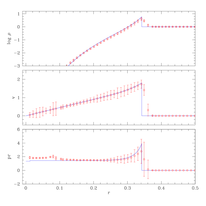
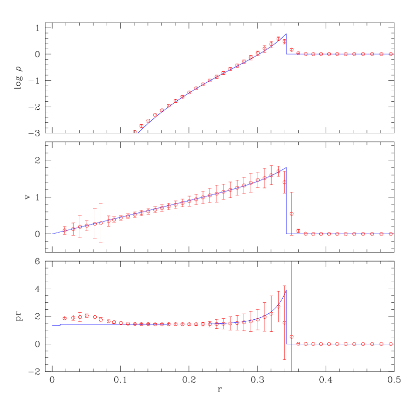
Figure 1: Angle-averaged density, velocity, and pressure profiles at time $t=0.063$ from two SPH simulations of a Sedov blast wave; the blue lines indicate the analytic solution. The two simulations use slightly different initial conditions, and consequently the results differ slightly as well; for example, the calculated density behind the shock generally falls below the analytic value in the first simulation but above the analytic value in the second. See §4.1 in the text for further discussion.

Figure 1 shows the angle-averaged density, velocity, and pressure profiles taken at time $t=0.063$ from two Sedov explosions simulated using SPH. The two simulations differ only in the specific arrangement of particles used for the initial conditions; both sets of initial conditions were constructed from concentric spherical shells of particles, but the simulation shown in the right-hand plot had an inner shell radius ten times smaller than the inner shell radius used in the left-hand simulation. Each circle represents the mass-weighted mean flow quantity and location of particles in a single radial bin (where the width of each bin is 0.01). The error bars indicate one (mass-weighted) standard deviation around the weighted mean. The blue line indicates the analytic solution.

Part of the scatter in the particle densities and pressures at a given radius arises from uncertainties in the initial density profile. One drawback of SPH is that there is an intrinsic scatter in the density because of the dependence and variability of the smoothing length. Even if we fine-tune the initial model, the scatter will develop after a few timesteps. This scatter places a low-level perturbation to seed any convection. In most past simulations by SNSPH, this scatter had a 1-sigma error of 10% in the density. Although we now can reduce this scatter somewhat, it is still an issue with SNSPH calcuations. In stellar collapse, it is likely that the explosive burning just prior to collapse produces density perturbations at this level. If anything, the 10% scatter in our SPH set-up is on par with what we expect to be the true initial conditions. We have run calculations with a factor of 2 larger scatter, and it did not alter our convection or mixing results in the explosion calculation.

The two simulations also illustrate the effect of different initial particle arrangements on flow quantities throughout the simulation. Decreasing the radius of the innermost shell of particles results in a pressure profile that more accurately matches the analytic solution behind the shock front. Additionally, the density profile in the left-hand simulation falls slightly below the analytic value, while the density in the right-hand simulation is slightly higher than the analytic value. This variation demonstrates the sensitivity of SPH to the initial arrangements of particles in a simulation and emphasizes the importance of carefully constructing and testing sets of initial conditions.

From these calculations, we see that the SPH calculation produces fairly accurate shock velocities, but densities and pressures that are low (although the shock entropy is more accurate). These errors decrease with resolution but, in most of our core-collapse simulations, we have not yet reached a satisfactory convergence on the shock modeling. A more realistic, but less standard, test would have a shock traverse a density gradient instead of a constant density profile. Fryer et al. (2006) compares the results of such a test for a number of coding techniques, including this SNSPH code.

4.2 Galactic Center Shocks

The Sedov blast wave tests a single, spherically-symmetric strong shock. In a grid code, such a test calculation can be easily fine-tuned by using a spherically symmetric grid and using solvers that assume that the shock front will be parallel to the grid. Unfortunately, the supernova problem does not have such a well-defined shock and fine-tuning the solver for a parallel grid may well give a worse answer for the specific case of stellar collapse.

Devising a test for more chaotic shocks is difficult. Few have analytic solutions. Instead we present here an experimental test. The X-ray emission in the Galactic center has been recently studied in detail by the Chandra X-ray Observatory. This X-ray emission is dominated by a point source Sgr A^∗, believed to be a $3.7\times 10^{6}$ M_⊙ black hole (see Ghez et al. 2005, although Rockefeller et al. 2004 used a $2.6\times 10^{6}$ M_⊙ black hole) accreting the gas around it. But there is also a diffuse X-ray component which is believed to be produced by colliding gas in the Galactic center. This gas arises from stellar winds from 25 wind-producing stars. Since the X-ray emission is proportional to the square of the density of the gas, it is an ideal probe of the shocks in this system. As with any experimental test, there are uncertainies both in the initial conditions, the relevant physics, and the final measurement. Let’s consider both of these sets of uncertainties.

The initial conditions for this problem consist of 25 mass-losing stars (the contribution by the other stars near the Galactic center is negligible). Indeed, most of the wind matter arises from the 7 strongest wind sources. Table 1 (from Rockefeller et al. 2004) gives the positions, wind velocities, and mass-loss rates for all of these stars. Although the x and y (projected) positions are fairly well-known, the z (radial) positions are completely unknown. Rockefeller et al. (2004) found that taking extreme positions for the coordinates of these wind sources led to 15% variation in the X-ray flux. The other uncertainties lie in the wind velocities and mass-loss rates of each of these stars. Those stars for which we have observations of the He I line emission have wind velocities that are known, but for many stars, the wind velocities and their associated mass-loss rates are merely estimated (see Rockefeller et al. 2004 for details). However, the total mass lost in winds as well as the wind structure of the 7 dominant mass-losing stars are better constrained, so despite uncertainties in some of the stars, these initial wind conditions appear sufficiently constrained to use this experiment. And with time, these initial conditions will only become better known.

The relevant physics for this problem is fairly straightforward. The equation of state is accurately modeled by an ideal gas with a $\gamma=5/3$ power law. The gravitational force is dominated by the central black hole (see Rockefeller et al. 2004 for details). It is unlikely that global magnetic fields will be sufficiently strong to play a role in the diffuse X-ray emission (although they may effect the X-ray emission from the point source). At the temperatures and densities that these shocks produce, the dominant components of the continuum emissivity are electron-ion ($\epsilon_{ei}$) and electron-electron ($\epsilon_{ee}$) bremsstrahlung (Rockefeller et al. 2004 used the standard simplified representations for these emission processes). The only other physics that need be considered is the possibility of surrounding molecular clouds which confine the wind material. But these clouds mostly affect the spatial distribution of the X-ray emission. This effect is limited to the low-level contours of the X-ray emission, and hence does not effect the total X-ray emission considerably.

The strongest observational constraint we can currently apply from the Galactic center is the total diffuse X-ray luminosity. Observations currently place this luminosity at $(7.6^{+2.6}_{-1.9})\times 10^{31}{\rm ergs\,s^{-1}\,arcsec^{-2}}$. In principal, the X-ray contours can be used as a constraint, but the low-level contours are very sensitive to the positions of the stars and the structure of the surrounding gas. At this time, more detailed tests of this multi-shock problem are best limited to code comparisons. We provide 3-dimensional density and energy plots on our website (http://qso.lanl.gov/$\sim$clf/codetest) for comparison.

4.3 Adiabatic Collapse

The adiabatic collapse of an initially isothermal spherical cloud of gas has been used in several investigations of SPH codes with gravity (Steinmetz & Müller 1993; Thacker et al. 2000; Springel et al. 2001, Wadsley et al., 2004). We follow the units used in the first presentation of this problem (Evrard, 1988). With $G=M=R=1$, the initial density distribution is:

$$\rho(r)=M/(2\pi R^{2})r^{-1}=(2\pi r)^{-1}.$$ (41)

where $M$ is the total mass of the system within the cut-off radius $R$.

The initial internal energy of the system is chosen as $0.05GM/R$, with the adiabatic index $\gamma=5/3$. The initial physical density distribution was applied to a grid with hexagonal symmetry using the technique of Davies, Benz & Hills (1992). The gravitational potential was smoothed with a Plummer softening of 0.01 R (Plummer 1911). The SPH kernel was initially set to give roughly 60 neighbors for each particle, and the SPH smoothing length was allowed to evolve within the constraints of $h_{max}=150$ and $h_{min}=30$.

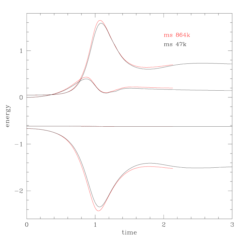
Figure 2: The time evolution of thermal, kinetic, total and gravitational potential energies during the adiabatic collapse of an initially isothermal gas sphere for SPH calculations with 43,000 and 864,000 particles. This figure may be compared with the 1-dimensional PPM and 3-dimensional SPH calculations from Figure 6 of Steinmetz & Müller (1993).

We show results for simulations with 47,000 particles, and with 864,000 particles in Figure 2. The 864k simulation conserves total (kinetic + internal + potential) energy to the 1% level at t=2.1 using 1475 timesteps. The 47k simulation conserves total energy to 1.2% at t=3.0 using 600 timesteps. Our version of SPH gives very similar results to the version of SPH presented in Steinmetz & Müller (1993). As we increase resolution, our solution approaches the solution from their 1-dimensional PPM simulation which has a much higher effective resolution per dimension.

4.4 Binary Orbits: Testing Angular Momentum Conservation

One of the true strengths of the SPH method is that it can conserve both linear and angular momentum at the same time. This feature makes SPH an ideal technique in modeling binary interactions and rotation in core-collapse calculations. However, even though SPH conserves angular momentum between particle interactions and hence is globally conserved, a code may still numerically transport that angular momentum and one must test both the conservation and artificial transport before running simulations that depend heavily on angular momentum. In this subsection, we will focus on a test to determine the level at which angular momentum is conserved in our SPH code. We first show how the SPH equations lead to angular and linear momentum conservation. To test the actual application of these equations, we follow the evolution of a close binary system for over 15 orbits. This test allows an ideal measurement of the angular momentum conservation in a system. We end with a discussion of methods to test the importance of numerical angular momentum transport.

Angular momentum is conserved by noting that the forces are always directed along a line joining the particle pairs (eq. 18). Recall that the torque on a given particle $i$ by particle j is $\tau_{i,j}=\overrightarrow{r_{i}}\times\overrightarrow{F_{i}}$ where $\overrightarrow{r_{i}}$ is the vector from a reference point to particle $i$ and $\overrightarrow{F_{i}}$ is the force on particle $i$ due to particle $j$. Figure 3 shows our particle pair. Because the acceleration of our particles is along the line joining these particles, the torque on any two particles are equal in magnitude, but opposite in sign, balancing each other and leading to angular momentum conservation:

$$\tau_{i}=r/sin(\theta_{i})F_{i}sin(\theta_{i})=rF_{i}=r/sin(\theta_{j})F_{j}sin(\theta_{j})=-rF_{i}=-\tau_{i},$$ (42)

where we have used from equation 18 the relation $F_{i}=m_{i}(d\overrightarrow{v}_{i}/dt)_{j}=-m_{j}(d\overrightarrow{v}_{j}/dt)_{i}=-F_{j}$. The SPH equations strictly conserve linear and angular momentum.

To test how well such a formulism works in an applied problem, we consider the problem of a binary system in an extremely close orbit. We use two equal-massed stars with a semi-major axis of $2\times R_{\rm star}$. The initial stars were evolved for the equivalent of 6 orbits as single stars before being placed into this binary system. These two single stars were then placed in a close orbit around each other with spin periods set to the orbital period. This close orbit was chosen to study the angular momentum conservation in an extreme situation, but bear in mind that the stellar radius is roughly 20% larger than its Roche-radius, so as time proceeds, the stars will gradually lose matter. But since we run our simulations only for 18 orbits, we shall see that this is only a large effect at late times. Such a binary test simulation, but under less extreme orbital conditions, has been done with grid-based codes (e.g. Motl, Tohline, & Frank 2002) and we compare, where possible, with these simulations.

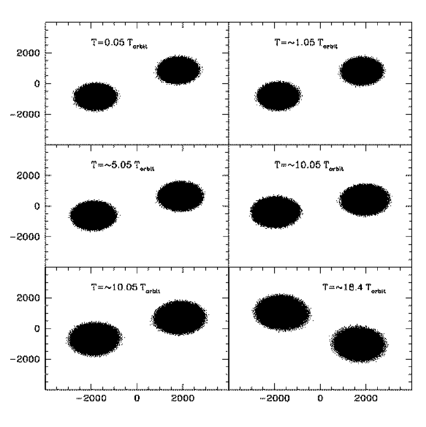
Figure 4: Snapshots in time of the evolution of a binary system put just inside the Roche-radius separation. The particles shown are limited to a slice in the orbital plane, $-50<z<50$ in code units. Although most aspects of this problem are scalable, the actual problem is of two 16 M_⊙ stars with a separation of $4\times 10^{11}$cm placed in a near circular orbit.

Fig. 4 shows a slice ($|z|<50$ code units) in particle distribution for our binary system at 6 different times (roughly corresponding to the same point in the orbit except for the last time which corresponds to our final time dump). No particles leave the system (all particles remain bound to their star). However, because they are both overfilling their Roche-radius, the stars slowly expand with time, preferentially building up mass at the L1 Lagrange point. Fig. 5 shows the angular momentum as a function of time (bottom) and the orbital radius as a function of time (top) for the binary. The orbital radius oscillates because of a slight error in our choice of the orbital velocity in the initial condition. As we shall see, this ultimately causes the code to break. As we are using our tests to find weaknesses in the code, we believe this initial deviation from a circular orbit a nice additional test to the code. In addition, the orbital serpartion drops by nearly 1% after 18 orbits. This is mostly because material is piling up at the L1 point, causing the mass-weighted center of the stars to move slightly toward that Lagrange point. The orbital angular momentum remains much better conserved, deviating by only 0.01% after 15 orbits. This occurred with fairly lenient error tolerances on our MAC and no tuning of the code to address this problem. The lack of angular momentum conservation is a result of the distortion in the stars coupled to the lenient tolerances on the MAC (leading to growing errors in the gravitational acceleration). A circular orbit initial condition, or more stringent MAC tolerances could reduce this error. In comparison, the tuned simulations (the best we have seen thusfar by grid codes) by Motl et al. (2002) using grid methods found deviations of nearly 0.08% after only 5 orbits!

But not all of the expansion of the star is due to Roche-Lobe overflow. The tidal forces in this problem lead to friction that, with our artificial viscosity, causes the star to heat up and expand. This numerical artifact of codes with artificial viscosity leads to poor energy conservation. Many fixes exist (Balsara 1995; Owen 2004), but in most of the problems we have study, shocks develop quickly and are fairly extensive. For such problems with widespread shocks, these fixes do not seem to make a noticeable difference in the simulation and we do not include these techniques in any of the current simulations done with this code. Figure 6 shows the absolute value of the energy components as a function of time in units of the total energy. The potential (dotted line) and, because the stars are bound, the total (solid) energies are negative. The magnitude of the total, potential, and thermal energy all decrease with time because of the expansion of the stars. The kinetic energy, the primary diagnostic of the orbits, remains relatively constant (which is a simple reflection of the conserved angular momentum and the rough conservation in the orbital radius). Because of the high artificial viscosity in this simulation, the system gains 10% of its total energy after 10 orbits, and another 15% after 18 orbits. The artificial viscosity terms were reduced slightly from our standard set: $\alpha=1.0,\beta=2.0$, but varying this value did not change our momentum conservation noticeably. At the expense of shock modeling, we could decrease the artificial viscosity to reduce the errors in the energy conservation.

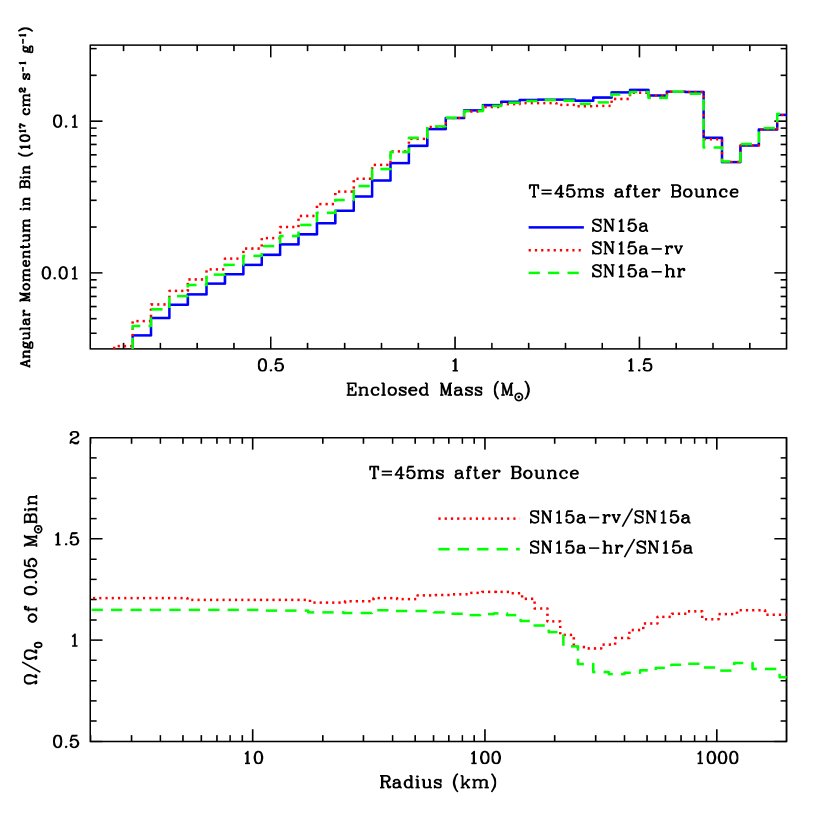
Figure 7: Top: Angular momentum versus enclosed mass for a rotating collapsing star (Fryer & Warren 2004). The 3 lines represent the standard model (solid line), a model using an artificial viscosity reduced by a factor of 10 (dotted line), and a high resolution model (dashed line). Bottom: The ratio of these angular velocities: reduced viscosity/standard (dotted line) and high resolution/standard (dashed). The answer does not change by more than 10-20% when reducing the artificial viscosity, and it is unlikely that we are off by more than that value for the angular momentum in our simulations.

The artificial viscosity in SPH, acting like any viscosity (real or numerical), leads also to angular momentum transport. Fryer & Warren (2004) worried about this specific effect in their collapse calculations of rotating supernovae. Fortunately, numerical viscosity can be controlled and its effects can be understood. Figure 7 shows the angular momentum profile versus mass (top) for a standard model (1 million particles - solid line), a model with high resolution (5 million particles - dashed line) and a module with the artificial viscosity reduced by a factor of 10 (dotted line). The high resolution and reduced viscosity simulations reduce the effect of numerical angular momentum transport (in the reduced viscosity simulation, by nearly a factor of 10). The bottom panel of figure 7 shows the ratio of angular velocities of the two modified simulations with respect to the standard simulation. What we find is roughly 20% more angular momentum in the core. With our extreme reduction in viscosity, this corresponds to the maximum errors in the angular momentum transport caused by numerical viscosity. This result eased the concerns Fryer & Warren (2004) had regarding the effects of numerical viscosity on the angular momentum transport in their collapse calculations.

Both the conservation and numerical transport of angular momentum must be studied when modeling rotating systems. In most cases, SNSPH exhibits very few numerical errors with angular momentum and is an ideal technique for rotating problems.

4.5 Flux-Limited Diffusion Test

The flux-limited diffusion scheme described in §2.3 follows the radiation diffusion between a particle and all of its SPH neighbors. This scheme, originally developed by Herant et al. (1994), uses the neighbor list generated to evaluate SPH forces and can be parallelized using the same techniques used to parallelize SPH. Its major limitation on the scalability arises from converting from the flux-limited diffusion algorithm to the free-streaming solution. At this point, a global sum must be made over all processors, placing a synchronization point in the code. But, in general, it is both fast and easy to implement.

Testing radiation transport schemes in general would, and has, comprised many papers in itself. Here we focus on a simple test comparing the SPH flux-limited scheme to a 1-dimensional grid-based flux-limited transport scheme. This test does not prove the applicability of flux-limited diffusion to the supernova problem, but it does show that our scheme for putting flux-limited diffusion into SPH does work.

For the initial conditions of this test, we use a spherically-symmetric neutron star atmosphere (material below $10^{14}$ g cm^-3) for a neutron star roughly 130 ms after bounce. We map this structure onto our SPH particles, setting up the particles in a series of spherical shells. The shells are produced by placing particles randomly on a sphere and using repulsive forces to evenly separate these particles within a predetermined tolerance. We make a similar setup in a 1-dimensional grid using one zone per shell of SPH particles. With this setup, we minimize the differences between the density and temperature structure of our 1- and 3-dimensional models. We determine the trapping radius to be 25 km. Below this radius, we set the electron neutrino fraction ($Y_{\nu_{e}}$) to 0.15 with a mean energy of 10 MeV. Above this radius, $Y_{\nu_{e}}$ is set to zero.

Our test focuses on the neutrino transport alone; we evolve only the electron neutrino fraction with time and hold the density, temperature, and electron fraction fixed. We allow no new neutrino emission. The flux arising from our neutrino trapping radius versus time for both our 1-dimensional grid simulation and our 3-dimensional SPH calculation is plotted in figure 8. The initial flux of the SPH calculation is higher, since the neighbors of any particle extend beyond the equivalent of an adjacent cell for the 1-dimensional calculation. In general, the luminosity for both these calculations agree to better than 3%.

More detailed tests are required to truly trust this transport scheme. Sufficiently complex tests can not be solved analytically and we are currently developing a set of comparison calculations using Monte Carlo (with its well-defined errors) as a solution (Hungerford et al. 2006).

5 Conclusions

The SNSPH code is built upon the parallel tree code of Warren & Salmon (1993,1995). This code has proven extremely portable and scalable (beyond 1000 processors) on a number of computer architectures from large supercomputers — the Advanced Simulation and Computing Program (e.g. Red, Pink, Q) and National Energy Research Scientific Computing Center (e.g. Seaborg) — to local Beowulf clusters — e.g. Space Simulator —. SNSPH uses the Benz version (Benz 1989) of Smooth Particle Hydrodynamics to model the Euler equations. A number of equations of state have been implemented to close these equations, from ideal and perfect gas equations of state to planetary equations of state (Benz, Slattery, & Cameron 1986) to the equation of state cocktail used to model core-collapse (Herant et al. 1994). SNSPH also includes an explicit flux-limited diffusion scheme to moderate neutrino transport (Herant et al. 1994, Fryer & Warren 2002). This transport scheme is even now being modified to model photon transport.

Although the focus of SNSPH has been to study stellar collapse (Fryer & Warren 2002,2004; Fryer 2004) it has also been adapted to model stellar explosions (Hungerford et al. 2003, 2005) and the Galactic center (Rockefeller et al. 2004, 2005) with a list of ongoing projects that spreads even further to planet formation and cosmology.

But, as with any computational technique, this code has both advantages and disadvantages. We have presented a number of tests of this SNSPH code. These test problems go beyond the standard “shock” tests (Sedov, Sod problem, shock tube) common in most test suites and include tests of the broad range of physics modelled in core-collapse. Our tests mark just the beginning set of tests SNSPH must pass if it is to become a multi-purpose radiation hydrodynamics code.

Even so, we can already outline the strengths and weaknesses of the SNSPH technique. The particle based scheme allows modellers to preserve many advantages of a Lagrangian scheme in turbulent flows where typical grid-based Lagrangian cells become tangled. We have shown that the hydrodynamics scheme conserves both total energy and momentum. Our scheme is easily modified to include a wide variety of equations of state and external forces and the transport scheme can be modified to model the transport of photons as well as neutrinos. The advantages include:

• Lagrangian technique allows the resolution to follow the mass. This is ideal for problems that cover a large range of spatial scales, but that focus the mass in one place (e.g. supernova explosions). It is also ideal for problems where the area of interest moves with time (e.g. in neutron star kicks and in binaries).

• The Lagrangian scheme also avoids any numerical diffusion (either heat or elemental abundances) that plague any Euler scheme during the advection step. Such artificial diffusion can lead to disastrous results in problems where the abundances must be tracked exactly (e.g. nucleosynthesis issues in supernova explosions) and abundance gradients are large. The same is true for problems where the temperature gradient is large.

• SPH conserves angular momentum and linear momentum at the same time.

• The explicit flux-limited diffusion transport scheme scales well (for transport schemes).

The disadvantages of the particle based method are few and can be summed up in three limitations with respect to core-collapse supernovae:

• SPH initial conditions tend to have small perturbations on the 5-10% level that will artificially seed convection. Such perturbations are difficult to reduce completely and their effects must be understood when interpreting simulation results.

• The artificial viscosity term added to model shocks does not work as well as Riemann methods when the shock moves along the grid. However, when the shock is not so well behaved, we believe (and propose a test for comparison) that SPH behaves as well as most grid codes. The artificial viscosity also leads to both an artificial angular momentum and artificial heating term. In shear flows, such numerical effects can lead to unrealistic heating. We have shown (Fryer & Warren 2004) that this is not an issue for even our fast-rotating supernova cores.

• Transport schemes are generally designed for grid-based codes. The flux-limited transport scheme in this code works at a basic level, but more sophisticated schemes have not been incorporated into SPH, and much more work must be done to prove that more sophisticated schemes can be added smoothly.

No code is ideal for all problems. Without the development of a more sophisticated transport scheme for SPH (whether it be a direct discretization method such as $S_{n}$ or a monte-carlo technique), our SNSPH code will not be able to model the detailed neutrino transport many believe is necessary to get a final solution to the core-collapse supernova problem. New transport schemes applicable for SPH are being pursued and the current dearth of schemes may not prove a long-term limitation. There are many problems that are most easily solved with a Lagrangian technique: from supernova explosions to binary mergers to galaxy collisions. SNSPH is ideally suited for these problems and has the versatility to adapt to these problems quickly. With other problems, such as black hole accretion disks, the gas accretion during the formation of Jovian planets or the complex shock structure in the Galactic center, SNSPH has its advantages and disadvantages over grid-based codes. SNSPH is a powerful tool in developing a solution to these outstanding astrophysical problems.

Acknowledgments This work was funded under the auspices of the U.S. Dept. of Energy, and supported by its contract W-7405-ENG-36 to Los Alamos National Laboratory, by a DOE SciDAC grant number DE-FC02-01ER41176 and by NASA Grant SWIF03-0047-0037. The simulations were conducted on the Space Simulator and ASC PINK at Los Alamos National Laboratory.

Table 1: Parameters for Galactic Center Wind Sources

Star	x	y	z1	z2	v	M⊙
	(arcsec)	(arcsec)	(arcsec)	(arcsec)	(km s-1)	(${10}^{-5}\;M_{\odot}$ yr-1)
IRS 16NE	0$-$2.6	0+0.8	0+2.2	0+6.8	0string550	09.5
IRS 16NW	0+0.2	0+1.0	0$-$8.3	0$-$5.5	0string750	05.3
IRS 16C	0$-$1.0	0+0.2	0+4.5	0+2.1	0string650	10.5
IRS 16SW	0$-$0.6	0$-$1.3	0$-$2.5	0$-$1.2	0string650	15.5
IRS 13E1	0+3.4	0$-$1.7	0$-$0.3	0+1.3	1,000	79.1
IRS 7W	0+4.1	0+4.8	0$-$5.5	0$-$2.8	1,000	20.7
AF	0+7.3	0$-$6.7	0+6.2	0$-$1.2	0string700	08.7
IRS 15SW	0+1.5	+10.1	0+8.7	0+0.3	0string700	16.5
IRS 15NE	0$-$1.6	+11.4	0+0.7	0$-$1.1	0string750	18.0
IRS 29N	0+1.6	0+1.4	0+8.3	0+3.2	0string750	07.3
IRS 33E	0+0.0	0$-$3.0	0+0.6	0+6.0	0string750	07.3
IRS 34W	0+3.9	0+1.6	0+4.0	0$-$4.8	0string750	07.3
IRS 1W	0$-$5.3	0+0.3	0$-$0.2	0$-$4.5	0string750	07.3
IRS 9NW	0$-$2.5	0$-$6.2	0$-$3.5	0$-$4.1	0string750	07.3
IRS 6W	0+8.1	0+1.6	0+3.1	0$-$0.4	0string750	07.3
AF NW	0+8.3	0$-$3.1	0$-$0.1	0$-$2.4	0string750	07.3
BLUM	0+9.2	0$-$5.0	0$-$4.1	0+0.2	0string750	07.3
IRS 9S	0$-$5.5	0$-$9.2	0$-$5.9	0$-$0.3	0string750	07.3
Unnamed 1	0+1.3	0$-$0.6	0$-$5.4	0+5.5	0string750	07.3
IRS 16SE	0$-$1.4	0$-$1.4	0$-$8.1	0$-$5.7	0string750	07.3
IRS 29NE	0+1.1	0+1.8	0+3.1	0$-$3.1	0string750	07.3
IRS 7SE	0$-$2.7	0+3.0	0+2.3	0$-$5.4	0string750	07.3
Unnamed 2	0+3.8	0$-$4.2	0$-$8.5	0+4.5	0string750	07.3
IRS 7E	0$-$4.2	0+4.9	0+8.6	0+1.3	0string750	07.3
AF NWW	+10.2	0$-$2.7	0$-$1.9	0+3.9	0string750	07.3

Figure 3: Diagram of the force interactions between a pair of particles in an SPH calculation. The torque on particle i from particle j viewed from an arbitrary reference point p is $(r/sin\theta_{i})F_{i}sin\theta_{i}$. Using $F_{i}=-F_{j}$ from §2, one can easily show that the torque on particle $i$ from particle $j$ is equal, but opposite, to the torque exerted on particle $j$ by particle $i$.

Figure 5: Top: Mass-averaged orbital separation (in units of the initial separation) versus time (in units of orbital periods) for the binary simulation. The oscillations arise from errors in the initial orbital velocities. As mass begins to fill the Lagrange point, the mass-averaged orbital separation begins to decrease. Bottom: total angular momentum (in units of initial total angular momentum) versus orbital time. The total angular momentum is conserved to better than 0.01% for 15 orbits.

Figure 6: Absolute energy versus orbital time. The total (kinetic+thermal+potential) energy (solid line) and potential energy (dotted line) are both negative (the system is bound). Artificial viscosity causes the star to heat up, but because it then expands, the total thermal energy (dashed line) actually decreases with time. The kinetic energy (dot-dashed line), however, remains relatively constant, a reflection of the angular momentum conservation.

Figure 8: Neutrino luminosity as a function of time for our test of the flux-limited diffusion algorithm in SNSPH. The dotted line shows the results using SNSPH and the solid line is the result from the 1-dimensional flux-limited diffusion code. Due to the smoothed nature of the algorithm in SPH, there is an initial spike in the SPH result. However, after the first few milliseconds, the two results converge and agree to less than a percent.

References

- Balsara (1995) Balsara, D.S. 1995, J. Comput. Phys. 121, 357
- Benz (1984a) Benz, W. 1984, A&A, 139, 378
- Benz (1984b) Benz, W. 1988, Comp. Phys. Comm., 48, 97
- Benz (1989) Benz, W. 1989, in “Numerical Modeling of Stellar Pulsation: Problems and Prospects, NATO Workshop, Les Arcs, France (1989), 269.
- Benz et al. (1989) Benz, W., Thielemann, F.-K., & Hills, J. G. 1989, ApJ, 342, 986
- Blinnikov, Dunina-Barkovskay, & Nadyozhin (1996) Blinnikov, S.I., Dunina-Barkovskaya, N.V., & Nadyozhin, D.K., 1996, ApJS, 106, 171
- Blondon et al. (2003) Blonding, J.M., Mezzacappa, A., DeMarino, C. 2003, ApJ, 584, 971
- Burrows et al. (2005) Burrows, A., Livne, E., Dessart, L., Ott, C., Murphy, J. 2005, submitted to ApJ, astro-ph/0510687
- Coker, R. et al. (2005) Coker, R. et al., in preparation
- Davies, Benz & Hills (1992) Davies, M.B., Benz, W., & Hills, J.G. 1992, ApJ, 401, 246
- EVRARD (1988) Evrard, A. E. 1988, Monthly Notices of the Royal Astronomical Society, 235, 911
- Fryer et al. (1999) Fryer, C.L., Benz, W., Herant, M., & Colgate, S.A., 1999, 516, 892
- Fryer & Warren (2002) Fryer, C.L., & Warren, M.S. 2002, ApJ, 574, L65
- Fryer & Warren (2004) Fryer, C.L., & Warren, M.S. 2004, ApJ, 601, 391
- Fryer (2004) Fryer, C.L. 2004, ApJ, 601, L175
- Fryer & Heger (2005) Fryer, C.L. & Heger, A. 2005, ApJ, 623, 302
- Fryer & Kusenko (2005) Fryer, C.L. & Kusenko, A. 2005, submitted to ApJ
- Fryer et al. (2005a) Fryer, C.L., Rockefeller, G., Hungerford, A., & Melia, F. 2005, accepted by ApJ
- Fryer et al. (2005b) Fryer, C.L., Rockefeller, G., & Young, P.A. 2005, submitted to ApJ
- Fryer et al. (2006) Fryer, C.L. et al. in preparation
- Ghez et al. (2005) Ghez, A.M., Salim, S., Hornstein, S.D., Tanner, A., Lu, J.R., Morris, M., Becklin, E.E., & Duchêne, G. 2005, ApJ, 620, 744
- Gingold & Monaghan (1977) Gingold, R. A., & Monaghan, J. J. 1977, MNRAS, 181, 375
- Herant et al. (1994) Herant, M., Benz, W., Hix, W. R., Fryer, C.L., & Colgate, S.A. 1994, ApJ, 435, 339
- Hix & Thielemann (1996) Hix, W.R., & Thielemann, F.K. 1996, ApJ, 460, 869
- Hungerford et al. (2003) Hungerford, A.L., Fryer, C.L., & Warren, M.S. 2003, ApJ, 594, 390
- Hungerford et al. (2005) Hungerford, A.L., Fryer, C.L., & Rockefeller, G. 2005, accepted by ApJ
- Hungerford et al. (2006) Hungerford, A.L., et al. 2006, in preparation
- Inutsuka (1994) Inutsuka, S. 1994, Memorie della Societa Astronomia Italiana, 65, 1027
- Inutsuka (2002) Inutsuka, S. 2002, Journal of Computational Physics, 179, 238
- Lattimer & Swesty (1991) Lattimer, J.M., & Swesty, F.D. 1991, Nuc. Phys. A, 535,331
- Lucy (1977) Lucy, L. 1977, AJ, 83, 1013
- Monaghan (1992) Monaghan, J. J. 1992, ARA&A, 30, 543
- Monaghan (1997) Monaghan, J. J. 1997, Journal of Computational Physics, 136, 298
- Monaghan (2005) Monaghan, J. J. 2005, Reports on Progress in Physics, 68, 1703
- Motl et al. (2002) Motl, P.M., Tohline, J.E., & Frank, J. 2002, ApJS, 138, 121
- Morris (1996) Morris, J. P. PhD thesis, Monash University, Melbourne
- Owen (2004) Owen, J.M. 2004, J. Comput. Phys., 201, 601
- Plummer (1911) Plummer, H.C. 1911, MNRAS, 71, 460
- Rasio (1999) Rasio, F. A. 1999, in the 5th International Conference on Computational Physics (ICCP5), held in Kanazawa, Japan, Oct 11-13 (Progress of Theoretical Physics).
- Rockefeller et al. (2004) Rockefeller, G., Fryer, C. L., Melia, F., & Warren, M. S. 2004, ApJ, 604, 662
- Rockefeller et al. (2005a) Rockefeller, G., Fryer, C. L., Baganoff, F.K., & Melia, F. 2005, accepted by ApJ
- Rockefeller et al. (2005b) Rockefeller, G., Fryer, C. L., Melia, F., & Wang, Q.D. 2005, ApJ, 523, 171
- Rockefeller et al. (2005c) Rockefeller, G., Fryer, C. L., & Melia, F. 2005, accepted by ApJ
- Salmon & Warren (1994) Salmon, J.K. & Warren, M.S. J. Comp. Phys., 111:136-155, 1994.
- Sedov (1982) edov, L.I. 1982 “Similarity and Dimensional Methods in Mechanics”, Mir Publishers, Moscow
- Springel et al. (2001) Springel, V., Yoshida, N., & White, S. D. M. 2001, NEW ASTRONOMY, 6, 79
- Springel, V. (2005) Springel, V. 2005, MNRAS, 364, 1105
- Steinmetz & Müller (1993) Steinmetz, M., & Müller, E. 1993, Astronomy and Astrophysics, 268, 391
- Suryadeep (2004) Suryadeep, R. 2004, A&A, 25, 103
- Taylor (1950) aylor, G. 1950, Proceedings of the Royal Society of London, Series A, Mathematical and Physical Sciences, Vol 201, No. 1065, 159.
- Thacker et al. (2000) Thacker, R. J., Tittley, E. R., Pearce, F. R., Couchman, H. M. P., & Thomas, P. A. 2000, Monthly Notices of the Royal Astronomical Society, 319, 619
- Tillotson (1962) Tillotson, J.H. 1962. Metallic equations of state for hypervelocity impact. General Atomic Report GA-3216, July 1962
- Timmes et al. (2005) Timmes, et al. in preparation
- Wadsley et al. (2004) Wadsley, J. W., Stadel, J., & Quinn, T. 2004, NEW ASTRONOMY, 9, 137
- Warren & Salmon (1993) Warren, M. S. & Salmon, J. K. 1993, in Supercomputing ’93 (Los Alamitos; IEEE Comput. Soc.), 12
- Warren & Salmon (1995) Warren, M. S. & Salmon, J. K. 1995, Computer Physics Communications, 87, 266
- Young et al. (2005) Young, P.A., Fryer, C.L., Hungerford, A.L., Arnett, D., Rockefeller, G., Meakin, C., & Eriksen, K.A. 2005, accepted by ApJ