11email: gieles@astro.uu.nl
2European Southern Observatory, ST-ECF, Karl-Schwarzchild-Strasse 2 D-85748 Garching bei München, Germany
3Department of Physics and Astronomy, University College London, Gower Street, London, WC1E 6BT
The luminosity function of young star clusters: implications for the maximum mass and luminosity of clusters
We introduce a method to relate a possible truncation of the star cluster mass function at the high mass end to the shape of the cluster luminosity function (LF). We compare the observed LFs of five galaxies containing young star clusters with synthetic cluster population models with varying initial conditions. The LF of the SMC, the LMC and NGC 5236 are characterized by a power-law behavior , with a mean exponent of . This can be explained by a cluster population formed with a constant cluster formation rate, in which the maximum cluster mass per logarithmic age bin is determined by the size-of-sample effect and therefore increases with log(age/yr). The LFs of NGC 6946 and M51 are better described by a double power-law distribution or a Schechter function. When a cluster population has a mass function that is truncated below the limit given by the size-of-sample effect, the total LF shows a bend at the magnitude of the maximum mass, with the age of the oldest cluster in the population, typically a few Gyr due to disruption. For NGC 6946 and M51 this suggests a maximum mass of , although the bend is only a 1-2 detection. Faint-ward of the bend the LF has the same slope as the underlying initial cluster mass function and bright-ward of the bend it is steeper. This behavior can be well explained by our population model. We compare our results with the only other galaxy for which a bend in the LF has been observed, the “Antennae” galaxies (NGC 4038/4039). There the bend occurs brighter than in NGC 6946 and M51, corresponding to a maximum cluster mass of . Hence, if the maximum cluster mass has a physical limit, then it can vary between different galaxies. The fact that we only observe this bend in the LF in the “Antennae” galaxies, NGC 6946 and M51 is because there are enough clusters available to reach the limit. In other galaxies there might be a physical limit as well, but the number of clusters formed or observed is so low, that the LF is not sampled up to the luminosity of the bend. The LF can then be approximated with a single power-law distribution, with an index similar to the initial mass function index.
Key Words.:
Galaxies: evolution – Galaxies: star clusters1 Introduction
The study of young extra-galactic star clusters has become a whole new field of research since the discovery of young massive clusters. The Hubble Space Telescope (HST) has made it possible to resolve these objects and to undertake systematic studies of the nature of these objects. Young clusters with masses in the range of our Milky Way globular clusters () have been found in merging galaxies like the “Antennae” (Whitmore & Schweizer 1995), interacting galaxies like M51 (Larsen 2000; Bastian et al. 2005b), starburst galaxies (Meurer et al. 1995; de Grijs et al. 2003a) and even non-interacting spiral galaxies (Larsen & Richtler 1999).
Recently, a relatively young and very massive cluster was discovered in the merger remnant NGC 7252 (Whitmore et al. 1993). Its (dynamical) mass was confirmed to be as high as (Maraston et al. 2004). This suggests that there are clusters that fill the gap between the mass range of star clusters and that of dwarf galaxies. However, it remains to be seen if every galaxy is able to produce such massive cluster or if there are physical limitations to the maximum mass of star clusters in different environments.
The LF of star clusters is a powerful tool when studying populations of star clusters. It indirectly gives us information about the underlying mass function (MF). Zhang & Fall (1999) showed for the young clusters in the “Antennae” galaxies that the cluster initial mass function (CIMF) can be well approximated by a power-law distribution: , with an exponent111Through the remainder of this work we will use for the exponent of the cluster initial mass function and for the exponent of the total cluster luminosity function. of . They derived the ages of the clusters using reddening-free parameters, which is necessary to extract the initial mass function from the total luminosity function. The exponent of the CIMF () is found to be close to in a wide range of galaxy environments down to masses of (de Grijs et al. 2003b). This resembles the mass function of molecular clouds (Solomon et al. 1987), consistent with clusters forming from molecular clouds. The LF can also be approximated with a power-law distribution: , where values for the exponent are found in a range of up till (Larsen 2002, hereafter L02; Whitmore 2003). In general the indices of the bright LFs are smaller (i.e. steeper) than the index of the CIMF (L02). One of the unanswered questions is whether the difference in slope between the mass function and LF have a physical meaning or if it is a result of different measurement techniques and artifacts like the contamination by stars at lower luminosities.
Whitmore et al. (1999) observe a distinct bend in the LF of young star clusters in the “Antennae” galaxies, where the slope faint-ward is shallower than the slope bright-ward of the bend. The exact slopes depend on the different ways of correcting for stellar contamination. They argue that this could be the progenitor turn-over of the peak that is observed in the luminosity function of old globular clusters which appears at , corresponding to a mass of . The difficulty with directly relating the LF to a CIMF is that the LF consists of clusters of different ages, and the mass-to-light ratio of clusters changes drastically when clusters age. Between and year, a star cluster of constant mass fades about 4 magnitudes in the -band. Recently, Mengel et al. (2005) observed the clusters in the “Antennae” galaxies in the Ks-band. They also find a double power-law behavior in the LF and argue that the mass function has a turn-over.
When there is no physical limit to the cluster mass or if there are not enough clusters to sample the CIMF up to any such limit, the mass of the most massive cluster will be determined by the total number of clusters and the slope of the CIMF (Hunter et al. 2003, hereafter H03). A similar idea was posed by Weidner et al. (2004), who suggest that the maximum cluster mass in a galaxy is determined by the star formation rate in that galaxy. It has not been shown yet in a large sample of galaxies that the most massive cluster is a result of size-of-sample effects. H03 only showed that this is the case in the SMC and the LMC. In this study we add M51 to the sample in order to see if the most massive object in this galaxy is also a result of size-of-sample effect or if there is a physical limit above which clusters cannot form in this galaxy. In addition, we use a method to relate a possible truncation of the mass function at the high mass end with the shape of cluster LF. To this end we introduce an analytical model to generate a cluster population and derive the LF for different cluster formation histories, disruption mechanism and CIMFs. We will show that even if the initial mass function of clusters is truncated, the brightest clusters in the sample may will still be determined by sampling statistics as found by Whitmore (2003) and L02.
The paper is organized as follows: In § 2 we introduce the data used for this study. In § 3 we present the masses and luminosities as a function of log(age/yr) for three galaxies in the sample. The LFs of cluster populations in five different galaxies are presented in § 4. We introduce in § 5 a cluster population model with which we can reproduce LFs based on various variables. The relation between maximum cluster mass and maximum cluster luminosity is discussed in § 6. A discussion in presented in § 7. The conclusions are presented in § 8.
2 Data
2.1 SMC and LMC
The ages and masses of clusters in the LMC and SMC were derived by H03 from ground based broad-band photometry. The data was taken by the Michigan Curtis Schmidt telescope by Massey (2002) and covers a large field of the LMC and SMC (11.0 kpc2 and 8.3 kpc2, respectively). Aperture photometry was used to derive and magnitudes. The colors and magnitudes were corrected for foreground reddening ( mag for the LMC and mag for the SMC). The ages and masses where derived by comparing the colors with the Leitherer et al. (1999) models. For more details on the data reduction and age derivation we refer to H03.
2.2 NGC 5236 and NGC 6946
Data for these two galaxies was taken from L02 and we refer to that paper for details about the data reduction and analysis. Briefly, clusters were identified on -band equivalent (F555W and F606W) HST/WFPC2 images and aperture photometry was carried out using a 3 pixels aperture. Cluster candidates were confirmed by a visual inspection of the images. For NGC 5236 and NGC 6946 there were 1 and 3 HST/WFPC2 pointings available, corresponding to 7.1 kpc2/53 kpc2, respectively.
2.3 M51
We used the age, mass and luminosity data of more than 1000 clusters in M51 found by Bastian et al. (2005b). Briefly summarized, aperture photometry was performed on F336W, F439W, F555W, F675W, F814W, F110W and F160W (roughly and ) images of the HST/WFPC2 and HST/NICMOS3 cameras. The magnitudes and colors were compared with the GALEV simple stellar population models (Anders & Fritze-v. Alvensleben 2003; Schulz et al. 2002) for different combinations of age and extinction. For detailed tests of the accuracy of the ages and the dependence on photometric errors and choice of models we refer to Bastian et al. (2005b). With 2 HST/WFPC2 pointings we cover 69 kpc2 of the inner region of the galaxy.
3 Masses and luminosities at different ages
3.1 Maximum masses at different ages
3.1.1 Predictions
The most direct way to study a possible truncation of the cluster mass function at the high mass end is to look at the masses of clusters as a function of the logarithm of the ages. When the cluster initial mass function (CIMF) is a power-law distribution () and not truncated, the maximum mass in the sample is purely determined by the size-of-sample effect. A single age distribution of clusters with a minimum mass consisting of clusters, will statistically have a maximum mass of . H03 showed that the maximum mass per logarithmic age bin should increase with log(age/yr) (assuming a constant cluster formation rate), since each logarithmic age bin corresponds to a longer time interval at older ages and hence more clusters. The number of clusters at higher log(age/yr) increases when assuming a constant cluster formation rate as: . So, the maximum mass of a sample of clusters formed with a constant cluster formation rate should increase with age () as
| (1) |
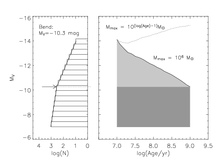
This is illustrated in Fig. 1. We statistically generated 10 000 clusters from a CIMF with exponent between log(age/yr) . In the left panel we plotted the results as a function of age and in the right-hand panel as a function of log(age/yr). The increase of the maximum mass predicted by Eq. 1 is only visible in the right-hand panel.

3.1.2 Observations
For three galaxies in our sample (SMC, LMC and M51) we have ages and masses of the individual clusters available from earlier studies. For details on the derivation of the ages we refer to § 2 and references therein. In Fig. 2 we plot the masses of the clusters as a function of log(age/yr) for the LMC (left), SMC (middle) and M51 (right). The completeness limit increases with age to higher masses due to fading of clusters caused by stellar evolution. The first impression may be that the unequal number of clusters in each age bin is incompatible with a constant CFR. However, the observed age distribution is a function not only of the cluster formation rate, but also of the detection limit and disruption of clusters. In addition, the age-fitting method yields some we irregularities. For examples all galaxies seem to have an over-density of clusters at log(age/yr)=7.2. This is a known fitting artifact (e.g. Gieles et al. 2005a). Therefore, the unequal number of clusters does not contradict a constant cluster formation rate.
The dashed line shows the slope of the predicted increase of the maximum mass, based on and Eq. 1. For the LMC and SMC the maximum cluster mass as a function of log(age/yr) can be well approximated by the size-of-sample prediction, as was shown already by H03. For M51 however, we see that for ages higher than year, there are more old high mass clusters predicted based on the size-of-sample effect than observed. However, the observations show that there are no clusters more massive than .

We also performed a linear fit to the maximum mass vs. log(age/yr). This is shown in Fig. 3. The most massive cluster in every log(age/yr) bin is indicated with a dot. The fit is shown with a full line. The LMC clusters older than log(age/yr)= 9.5 were not included in the fit, because there seems to be an age gap in the cluster distribution between 3 and 10 Gyr. For the SMC and LMC the fit is consistent with the size of sample effect and a CIMF exponent of , which was found already by H03 for the SMC and LMC. This is a rather steep slope for the CIMF and H03 showed that a fit to the first bins (log(age/yr) 8) yields a value of . It might be that for higher ages we are seeing a lack of old massive clusters. Note also that we here assume a constant formation rate of cluster and no mass loss of the clusters after formation. We will look at the effect of this assumption in § 3.1.3. For M51 we find a much shallower slope (0.26) than expected on account of the size-of-sample effect. If this slope was caused by the mass function, it should have an exponent of , which would be a much steeper slope than found in any other study. In fact, the CIMF has been determined for M51 by Bik et al. (2003) from young clusters and was found to be .

3.1.3 The effect of mass loss, infant mortality rate and variable cluster formation rates
In the conversion of the vs. log(age/yr) relation to a CIMF slope we assume that the clusters have not lost any mass after their formation and that the clusters were formed with a constant formation rate. In reality, only 10-30% of the clusters will survive the initial 10 Myr, clusters will lose mass due to stellar evolution (SEV) and tidal effects and the cluster formation rate (CFR) might not be constant at all. To quantify these effect, we generated a series of maximum masses consistent with the size-of-sample effect and a mass function exponent of , assuming a constant CFR. We then evolve each cluster mass as a function of its age according to the analytical formulas introduced by Lamers et al. (2005a). The mass of the cluster as a function of time can be well approximated by
| (2) |
where is the present mass of the cluster as a function of its age, is the initial mass of the cluster, is the fraction of remaining mass after mass loss due to stellar evolution has been subtracted. The value of is based on the GALEV models and analytically parameterized (see Lamers et al. (2005a) for details). is the disruption time of a cluster and is a dimensionless index indicating the dependence of the disruption time of clusters on the initial mass; . The value for is found to be 0.62 based on observations and -body simulations (Lamers et al. 2005b). Equation 2 describes the mass of a cluster as a function of time based on a variable final disruption time, taking mass loss due to stellar evolution and tidal evaporation into account.
We consider two scenarios: 1.) the SMC/LMC case and 2.) the M51 case. This is because the masses and disruption times are very different. For the SMC/LMC case we choose the maximum mass to be at log(age/yr) = 6.5, corresponding to the observed maximum mass at young ages. For the M51 case we choose a higher maximum mass; at log(age/yr) = 6.5, also based on the observed masses at young ages. We then assume a typical disruption time of clusters for the SMC and LMC of yr and yr for M51. The disruption times are based on the observationally determined values of Boutloukos & Lamers (2003) (SMC) and Gieles et al. (2005a) (M51) and the predicted values of Baumgardt & Makino (2003) (LMC). In Fig. 4 we show the slope of the cluster maximum masses as a function of log(age/yr) as predicted by the size-of-sample effect with a full line and the shallower increase after the clusters have been evolved in time for different scenarios. In the top panels we show the effect of stellar evolution and disruption for the two different scenarios. The disruption time of clusters in M51 is almost a factor of 15 shorter than for clusters in the SMC/LMC, but since the masses are higher and disruption is mass dependent (), the effect of the evolution is similar in both cases. Since this simple model can easily be extended to more realistic scenarios, we now include the effect of a high infant mortality rate in M51 in the bottom left panel of Fig. 4. Bastian et al. (2005b) estimate that 70% of the clusters does not survive the first 10 Myr, independent of their mass, so we increase the maximum mass for bins below 10 Myr with a factor of 3.3 to simulate the higher masses at young ages. The result is shown in the bottom left panel of Fig. 4. The inclusion of infant mortality makes the slope again slightly shallower. However, still not even close to the observed value. The last effect we consider, is a steady increase in the CFR. Since the maximum mass is proportional to the CFR, an increase in the CFR could result in more young massive clusters. To get to the slope of 0.26 as observed in M51 (bottom panel of Fig. 3), we apply an additional increase in the CFR. We assume that increase exponentially in time as CFR . To get to a slope of 0.26 as observed, we need , which means the CFR has increased a factor of 22 in the last few Gyr. M51 is in interaction with NGC 5195 which might have enhanced the CFR. In earlier work, however, we have determined the CFR increase to be in the order of a factor of 3-5 (Gieles et al. 2005a), which is in good agreement with independent determinations of the increase of the star formation rate for these kind of interacting systems, based on H measurements (Bergvall et al. 2003). Also, the increase in the CFR seems to be more in bursts rather than an exponential increase in time. A burst in the CFR will not affect the slope of Fig. 3, it will just show up as a peak. Worth noting is that the two peaks of M51 (Fig. 3) at log(age/yr)=7.8 and log(age/yr)=8.8. They coincide with the predicted moments of encounter with NGC 5195, 75 Myr and 450 Myr ago (Salo & Laurikainen 2000).
With this we show that part of the deviation from a slope of 1 in Fig. 3 is caused by stellar evolution, cluster mass loss due to tidal effects and infant mortality rate, but even the short disruption time and high infant mortality rate of M51 can not explain the observed shallow increase of the maximum cluster mass with log(age/yr) (Fig. 3, bottom), without assuming an unrealistically high increase in the CFR.

3.2 The cluster mass function
If the CIMF is truncated, the total MF of clusters should also show a truncation. As a check, we make the mass function, i.e. as a function of mass, for the SMC, LMC and M51. Since the detection limit cuts the sample at different masses (Fig. 2), we need to generate a mass and age limited sample. We choose minimum mass and maximum age combinations of and for the LMC, the SMC and M51 respectively. The resulting mass functions are shown in Fig. 5. The three mass functions where fitted with a single power-law, with variable slope and vertical scaling and with a power-law with exponential cut-off: , where the cut-off mass is an extra variable. This function is similar to the Schechter (1976) function, which will later be used to fit the luminosity function of clusters. The results of the truncated and untruncated power-law fits are compared by showing the ratio. The fit of the truncated power-law is over-plotted. For the SMC and LMC, however, this fit is similar to an untruncated power-law fit. The M51 mass function is better fitted with a truncated power-law. The values we find for are and for the SMC, LMC and M51 respectively. The value for M51 can be explained by mass dependent cluster disruption. If star clusters are formed with a CIMF with index , then the total mass function will have the same index, as long as the disruption time scale is longer than the maximum age in the sample. For the SMC and LMC the maximum age in the sample is yr, and the disruption time scale is yr (Baumgardt & Makino 2003; Boutloukos & Lamers 2003). For M51, however, the disruption time is shorter than the maximum age in the sample (Gieles et al. 2005a). Since the low mass clusters disrupt faster than the high mass clusters, the mass function gets shallower at older ages. Therefore we find that the MF has an index which is greater than , which is the index of the CIMF of M51 (Bik et al. 2003).

3.3 Maximum luminosities at different ages

Another way of looking at the size-of-sample effect, is by plotting the magnitudes of all clusters as a function of log(age/yr). In Fig. 6 we plot the magnitudes for the three cluster populations shown in Fig. 2. The advantage of looking at magnitudes instead of masses, although they are directly linked by the age and mass dependent magnitudes from SSP models, is that this figure helps to understand the LF, which will be discussed in § 4. The solid line indicates the fading of a single mass cluster based on the GALEV models, i.e. without tidal disruption. We shifted the starting magnitude to the brightest clusters at log(age/yr) = 6.5. The dashed lines now represent the luminosity of the most massive cluster as a function of log(age/yr) based on the size-of-sample effect and . From the GALEV simple stellar population we took the evolution of the magnitudes in time for a single mass cluster with some reference mass (), which is the maximum mass in the age range log(age/yr) 7. We then add extra mass to as a function of log(age/yr), following Eq. 1. The magnitude then depends on the age and the exponent of the CIMF as
| (3) |
where is a reference mass based on the observed maximum mass at young ages, is the maximum magnitude as a function of age, is the cluster age and is the exponent of the CIMF. The dashed lines represent the maximum luminosity based on the size-of-sample effect and Eq. 3, for . The lower luminosity increases with log(age/yr) for M51. This is since the clusters of M51 had to be detected in the F439W band in order to make the observed sample. Since clusters fade more rapidly in the filters bluer than the band, we miss some clusters at older ages and faint magnitudes. Since we are here only interested in the maximum luminosity, this will not affect our results. When the colors are used for cluster identification, these color differences have to be taken in to account.
The maximum luminosities of clusters in the LMC and SMC follow the dashed lines better than the fading line of the single mass cluster. The most luminous clusters in M51 seem to follow the fading of the single mass better then the dashed lines which are based on the size-of-sample prediction, which suggests that the underlying maximum mass is truncated at that mass.
Interestingly, Zhang & Fall (1999) made a similar plot for the luminosities of clusters in the “Antennae” galaxies (their Fig. 2). They also over-plot the luminosity evolution of single mass clusters in time. Their maximum luminosities seem to follow the models very well, which suggests that the maximum luminosity and hence the maximum mass of clusters in the “Antennae” galaxies does not follow the predicted size-of-sample relation of H03. All this suggests that the maximum mass of clusters in M51 and the “Antennae”galaxies are not determined by size-of-sample effects, but instead has a physical upper limit. The most luminous cluster in these galaxies however, in general being a young clusters due to the rapid fading in time of star clusters, is determined by size-of-sample effects. This agrees with what was found by Whitmore (2003) and L02, who showed that the maximum cluster luminosity in a galaxy depends on the total number of clusters in the galaxy above a certain luminosity. We will continue with this subject in § 6.
4 The luminosity functions of five galaxies
In this section we will present the LFs of (young) clusters in the SMC, LMC, NGC 5236, NGC 6946 and M51. For each galaxy the number of clusters as a function of was determined and a fit of the form was performed. The index of the magnitude distribution relates to the exponent of the LF as
| (4) |
where is the exponent of the LF (). In the following subsection we will first present the LFs and fit a power-law function to all cluster samples. In § 4.2 we will fit alternative functions and compare them with the power-law fits to determine the best fit model to the LFs. All results are summarized in Table 1.
4.1 The observed luminosity functions
4.1.1 SMC and LMC
The LFs of the SMC and LMC are based on the data of H03. The LFs are presented in the top two panels of Fig. 7. H03 report lower limit magnitudes of and for the LMC and SMC, respectively. Since the sample starts to be incomplete a bit bright-ward of the cut-off magnitude, we used very conservative completeness limits which are 1.5 mag brighter ( for the LMC and for the SMC). H03 only corrected for foreground reddening ( and 0.13 for the SMC and LMC respectively) and we have no extinction estimates for the individual clusters available. The detection limit is shifted the same amount as the LF when correcting for foreground extinction.
4.1.2 NGC 5236
The cluster sample of NGC 5236 is presented in L02. From the completeness tests presented in that paper and a distance modulus of 27.9, we found a 90% completeness limit of . We corrected the measured magnitudes for galactic foreground extinction based on Schlegel et al. (1998). We used the sample which had spurious sources removed after visual inspection. A foreground extinction correction of 0.218 mag was applied (Schlegel et al. 1998). The sharp cut-off at high luminosities is because some of the bright sources were saturated.
4.1.3 NGC 6946
The LF of clusters in NGC 6946 was presented in L02. We here use the sample of clusters where spurious sources have been removed after visual inspection. The 90% completeness limit, following L02, is = 22.0 and a distance modulus of 28.9 mag was used. The magnitudes were corrected for 1.133 mag foreground extinction based on Schlegel et al. (1998). The final LF can be seen in Fig. 7 (second from bottom). The LF contains more bright clusters than the previous ones. In addition the slope is slightly steeper. The fact that LFs with brighter clusters are better fitted with steeper power-laws was already noted by L02. In § 4.2 we will compare this fit with a double power-law fit and a Schechter function.
4.1.4 M51
For the LF of M51 the data from Bastian et al. (2005b) is used. We refer to this paper for detailed explanation on data reduction and source detection. Ideally, we select clusters for the LF independent of the applied age fitting routine. The best criterion for this would be to select on extended objects brighter than the 90% completeness limit in F555W. Since we only found reliable radius estimates for 305 objects, we selected the observed clusters that passed our fitting criteria from Bastian et al. (2005b), e.g. the sources that were well fit by a cluster model. Since one of our source selection criteria is that the object has to be above the 90% completeness limit in at least four bands, it is of importance which band we use. Comparing the SEDs for different ages of the GALEV models to the 90% completeness limits in all filters, we found that all clusters are always above our 90% completeness limit in F555W, F675W and F814W once they are detected in the F439W filter. If we apply the F555W 90% cut to the sample, our four-filter criterion will cut the sample sometimes because the source has to be visible in F439W as well, depending on the age. To be sure that for all ages our sample is limited by a cut in the F555W band only, we add the maximum color difference F439W – F555W from the GALEV models for clusters between and years to our F555W 90% completeness limit. This makes the cut in this filter 0.6 mag brighter than the 90% completeness limit of 22.7 mag. A distance modulus of M51 for 29.62 mag was used (Feldmeier et al. 1997) and a foreground extinction correction of 0.117 mag was applied (Schlegel et al. 1998). The LF for all clusters brighter than 22.0 mag in F555W is shown in the bottom panel of Fig. 7. As was the case for the LF of NGC 6946, we also fit a power-law which is steeper than the power-law CIMF index of Zhang & Fall (1999). We will consider different functions in § 4.2.

4.2 Fitting other functions to the luminosity functions
The brighter LFs of NGC 6946 and M51 are fitted with power-law functions with steeper slopes () than the fainter ones (). When a single power-law function is fitted to faint sides of the LFs of NGC 6946 and M51, we find similar values as for the SMC, LMC and NGC 5236. This suggests that the LFs turn over at the bright side, something what was found for the “Antennae” galaxies by W99 as well. In order to quantify the deviation from a single power-law, we fitted all LFs of § 4.1 with a double power-law function with variable break point and a Schechter function. The Schechter function is generally used for the LF of galaxies. It has a power-law nature on the faint end and a exponential drop at the bright side. In terms of magnitudes the Schechter function can be expressed as
| (5) | |||||
where is the magnitude in a band with central wavelength , is a normalization number, is the exponent of the power-law part of the LF and is the characteristic point of the function. is the equivalent of when using the Schechter function to fit the LF of galaxies.
To compare the different function fits for all five galaxies, we compare the reduced values of the different fits. In the top panel of Fig. 8 we show the ratio of for the five LFs. In the bottom panel we show the ratio of . The comparison shows that the LFs of NGC 6946 and M51 are better fitted with a function that drops at the bright end, although from the values in Table 1 and the comparison mentioned, a single power-law distribution can not be excluded with a high significance level.
In Fig. 9 we show the best fits to the LFs for all five galaxies, based on their results. The number of clusters is normalized to the observed area for fair comparison. We extrapolated the faint side of the LFs of NGC 6946 and M51 with a dashed line, this to show that these galaxies on the faint side have similar slopes as the other three cluster LFs. Another interesting fact is that NGC 6946 and M51 are on top, due to a high CFR. Therefore, they are also the only galaxies with cluster brighter than mag.


4.2.1 A closer look at NGC 6946 and M51


NGC 6946
To get a realistic idea of the location of the breakpoint, which we can compare with other galaxies, we need to take into account possible reddening. L02 did not determine reddening for the individual objects, but only mentions the Galactic foreground reddening. For the direction of NGC 6946 this is and we corrected the magnitudes of each cluster for this amount. The breakpoint was determined by fitting double power-laws with a variable breakpoint, exponents and normalization constant. We found the break to be at , with an exponent faint-ward of the break of and bright-ward of the break. The (foreground) extinction corrected LF with the double power-law fit can be seen in the top left panel of Fig. 10. W99 observe similar behavior for the LF of the “Antennae” galaxies. When they fit two power-laws, they find the breakpoint around , depending on the different samples they selected.
We also fitted a Schechter function (Schechter 1976), which has a more gradual bend and it is usually used to fit the LF of galaxies. This was also done for the clusters in the “Antennae” galaxies by W99.
The top right panel of Fig. 10 shows the result of the Schechter function fit to the (foreground) extinction corrected LF of NGC 6946. The bend in the Schechter function occurs at , which is 1.2 mag fainter than the of the “Antennae” galaxies (). The break point in the double power-law distribution occurs 1.2 mag fainter as compared to the “Antennae”.
M51
For M51, we corrected all magnitudes for the extinction values we acquired from the age fitting (see Bastian et al. (2005b) for details). This is important, since extinction effects might also affect the shape of the LFs. Bastian et al. (2005b) found that young clusters have on average higher extinction values than the older ones. L02 looked at the effect of differential extinction on the LF. He found that it makes the LF steeper, but only when there is already a cut-off in the mass distribution on the high mass end. If the mass function is not truncated, differential extinction does not affect the shape of the LF, since then still power-laws with the same index would be added, resulting in a power-law with that index. In case there is a relation between the luminosity and extinction, for example because we can see more intrinsically bright clusters, the bright part of the LF will be extinct ed more and this could result in a drop. To check this, we plotted the available extinction and luminosities from Bastian et al. (2005b) in Fig. 11. We averaged the extinction for different luminosity bins, and there is no relation between the two parameters. So the fits to the LF of M51 will have a higher reliability than the ones of NGC 6946, since there individual source extinction is not known.
When we fit a double power-law distribution, the location of the bend is at . The exponents on the faint and bright side of the breakpoint are and respectively (bottom left panel of Fig. 10). These values are very similar to those found for NGC 6946. The bottom right panel of Fig. 10 shows the result of a Schechter function fit to the M51 clusters. The exponent is and the bend is at .
The results of all fits to the LFs are summarized in Table 1. We added the values found by W99 for the “Antennae” galaxies as a comparison. The two exponents of the double power-law fits are very similar between NGC 6946, M51 and the “Antennae”. The breakpoint in the case of the double power-law fit, however, occurs about 1.2 mag brighter in the “Antennae” galaxies. The value for is also about 1 mag brighter compared to NGC 6946 and M51.
In the next section we will attempt to explain the shape of the LFs, in particular the bend observed for NGC 6946, M51 and the “Antennae” galaxies.
Table 1. Properties of the observed LFs.
| Galaxy | Break | Foreground extinction () | |||
| (mag) | (mag) | (mag) | |||
| SMC | - | - | - | 0.09 | |
| LMC | - | - | - | 0.13 | |
| NGC 5236 | - | - | - | 0.218 | |
| NGC 6946 | 1.133 | ||||
| M511 | - | ||||
| “Antennae”2 | - | ||||
| 1 Corrected for individual cluster extinction. | |||||
| 2 Values from W99 for their sample of extended sources. | |||||
5 A cluster population model
Our goal is to understand why we observe a bend in the luminosity function of NGC 6946, M51 and the “Antennae” galaxies and not in the other galaxies in the sample. The luminosity function (LF) of a star cluster population is a combination of multi-age cluster initial mass functions, which all have age dependent mass to light ratios. Clusters will lose mass in time due to stellar evolution and tidal effects, which will also affect the luminosity as a function of age. When there are no ages and masses of the individual clusters available, an alternative way to look at how the LF is built up is to model the LF based on various physical input parameters. In this section we will analytically generate the LF of a star cluster population.
5.1 Creating a synthetic cluster population
5.1.1 Set-up
The synthetic cluster population is based on an analytical model presented in Gieles et al. (2005a). In that work it was used to predict ages and masses of the cluster population of M51. The LF follows directly from these predictions since the combination of age and mass can be converted to luminosity using simple stellar population models.
The model creates a series of cells equally spaced in log() and log(). Then a CIMF and formation rate are chosen. Based on these choices each cell is assigned a weight (). To acquire a CIMF with exponent and a constant formation rate, can be written as
| (6) |
where is the weight assigned to a cell with age and mass , is the mass of the most massive cell in the simulation, is the age of the youngest cell in the simulation and is the exponent of the mass function. The weight is now a function of age and initial mass, where the most massive cell in the youngest bin has a weight of one, and corresponds to 1 cluster per log()–log() bin. This value is arbitrary and can change since later we will scale the total population to a different number. When is chosen, the weight depends on age and mass simply as: . When the cells are then binned in age, mass or luminosity, the weights of each cell are counted and the bin values now represent number of clusters. The main advantage of using these weight assigned cells spread equally in log() and log(), is that it would otherwise be very time consuming to generate cluster populations with a well sampled mass function; the amount of clusters needed for that is too high. Also, the number of points per bin is now constant and it is straight-forward to create a variety of populations with different formation rates, disruption time scales etc. in a short time. The model from Gieles et al. (2005a) is extended in this work to create LFs. To this end the age and mass dependent magnitudes of clusters are taken from the GALEV SSP models based on a Salpeter IMF. When generating a LF, the total weight of the cluster population is scaled to a realistic number of clusters. Then only bins with weights greater or equal to one are kept. In this way the predicted maximum luminosity follows directly from the model, depending on the number of clusters (=total weight) and the input variables.
5.1.2 Include stellar evolution and cluster disruption
In a recent study (Lamers et al. 2005a) it was shown that there is a simple analytical description of the evolution of the mass of a single cluster as a function of time (see Eq. 2, § 3.1.3). It takes into account the effect of mass loss due to stellar evolution, based on the mass loss predicted by the GALEV models and it includes mass loss due to tidal evaporation based on the -body results of Baumgardt & Makino (2003). The mass as a function of time according to these analytical formula agrees very well with the predictions from -body simulations (Lamers et al. 2005a). We assume stars of all type are lost due to disruption. In reality more low mass stars will leave the cluster. This might slightly affect the magnitudes as a function of time.
5.2 The luminosity function of a multi-age population
In the first step to understand the LF we generate an analytic cluster population with log() ranging from 7 to 9. Cells are spread equally in log() and log( space and weights are assigned to correct for the logarithmic binning in age and to create a mass function with . Cluster masses were assigned between 10 and . The upper mass was chosen unrealistic high, representing the lack of a physical upper limit to the most massive cluster in the mass function. The total weight is then scaled to 1000 clusters. In principle this step is not necessary, it tells us what the most luminous cluster in the sample is, since we will only use bins with values greater than one. (Note that due to the weights we use and the final scaling there are cells with weights much smaller than one.) Every cell is assigned a magnitude based on the GALEV models. The exponent of the resulting LF for this multi-age population is always . Although clusters with log() = 9 have faded considerably, the final LF is still an addition of power-laws with exponents of , with no limit to the maximum mass and hence the maximum luminosity. For this reason, changes in the formation rate as well as bursts will have no effect on the slope. Mass dependent disruption will slightly change the slope (§ 5.5.4).
5.3 The luminosity function without a maximum mass
When the CIMF is not truncated, the mass of the most massive cluster observed will increase with increasing log(age/yr) due to the size-of-sample effect (§ 3; H03). The most massive cluster will depend on age as , when . The dotted line in Fig. 12 takes this increase of the mass and the fading of the most massive cluster as a function of log(age/yr) into account. In two dex in age the maximum mass will also increase with two dex if the slope of the mass function is . This means that the most massive cluster at years will be a factor of 100 more massive and hence 5 mag brighter than the one at years. Since clusters fade about 4 mag between and years, these two effects almost cancel out. Not only the mass of the most massive cell will increase, but also the second most massive etc. Therefore, the LFs at different ages will all have clusters sampled between the detection limit and more or less the same maximum luminosity. So, the slope of the integrated luminosity function will be close to the slope of the CIMF for almost all luminosities, which we found already in § 5.2. This effect can be seen in Fig. 6 for the LMC and the SMC clusters. At all ages we find clusters between the detection limit and more or less the same maximum luminosity. Integration over all ages will yield a LF which has about the same slope as the mass function. This has always been assumed to be logic, but here we show that this is only the case when there is no maximum mass.
5.4 Truncation of the mass function
L02 has already shown that when generating a multi-age population with a truncation at the high mass side, the LF gets steeper. This can be understood as follows: when the underlying mass function is truncated at some upper mass, the brightest cluster will be the most massive cluster in the youngest age bin. This holds when the MF is sampled up to the truncation limit in the youngest age bin. The older clusters have faded due to stellar evolution. Hence at the brightest end of the LF only the youngest clusters will contribute. Going to fainter magnitudes, more and more ages will contribute to the LF. At the luminosity of the most massive cluster in the oldest age bin and fainter, all ages will contribute, and therefore the slope faint-ward of that brightness will be the slope of the CIMF, similar to what we found in § 5.2. This is illustrated in Fig. 12. The decreasing line in the right hand panel represents the luminosity of a 10 cluster between and years. The dark shaded region is where all clusters of all ages contribute to the same part of the LF. The light shaded region represent the clusters contributing to the bright end of the LF.
When there is a physical mechanism that does not allow clusters more massive than to be formed, there should be an observable bend at . With our model we now generate a cluster population with ages between and yr and masses between and and apply a detection limit at . The age range is based on the observed age range in M51. We excluded the clusters younger than log(age/yr)=7, since a large fraction of these clusters will not survive the first 10 Myr (e.g. Lada & Lada 2003; Bastian et al. 2005b). We apply no disruption or extinction. The total weight of this simulation is scaled to 1000 clusters. The brightest cluster now is the first bin at the bright side with a weight larger than 1. The resulting LF is shown in Fig. 13. The faint part has an exponent of , which is expected, since the underlying mass function has an exponent of . On the bright side the slope is steeper () and the break between the two power-laws is at mag, which is close to the magnitude of a cluster with an age of yr ( yr mag) . For NGC 6946 and M51 the observed break occurs at mag and mag respectively implies a maximum cluster mass of and . For comparison, the bend in the LF of the “Antennae” galaxies at corresponds to a maximum mass of , assuming the oldest cluster in the sample is also 3 Gyr. We also fit a Schechter function (Eq. 5) to the model as was done for the clusters in NGC 6946, M51 and the “Antennae” galaxies. When we fit this function to our model with and as variables we get a very good fit (see bottom panel of Fig. 13). As was the case with the Schechter fit to the observed LF of NGC 6946 and M51, the bend now occurs brighter than when breaking the LF into two power-law distributions. When comparing the bend points from the Schechter functions to the model, we find maximum cluster masses of , and for NGC 6946, M51 and the “Antennae” respectively. We note that the errors in the fitted break points and Schechter bends are large ( 0.5 mag), which corresponds to a factor 1.5 in mass. It is therefore hard to place a hard limit on the upper mass of the CIMF.


5.5 Impact of different initial conditions
Our assumed initial conditions of § 5.4 might affect our results and in particularly the location of a break in the LF. We therefore created several cluster populations, with different initial conditions.
5.5.1 Varying cluster formation rate
For simplicity we have taken the cluster formation rate (CFR) to be constant over 3 Gyr in § 5.4. Especially when comparing with M51 and the “Antennae” galaxies this might be an over simplification. We generated models with bursts in the CFR, as is probably more realistic for M51 (Gieles et al. 2005a). Bursts with increased CFRs of factors of 2-3 do not affect the location of the bend. For comparison with the LF of the “Antennae”, we increased the CFR the last 160 Myr, based on the results of Wilson et al. (2003). For a CFR which was 3/5/10 times higher the last 160 Myr as before, the bend occurs 0.3/1.5/1.8 mag brighter. This would make our observed maximum masses 1.3/4/5 times lower. As was shown in § subsubsec:massloss, the assumption of a constant CFR will always make it hard to directly compare the model with the data.
5.5.2 The stellar IMF
Our SSP models assume a Salpeter IMF. When a Kroupa was assumed, the corresponding mass derived from a bend in the modeled LF will be about a factor of 2 lower. To explain the bend location in M51, NGC 6946 and the “Antennae” galaxies, our derived maximum masses will also be a factor of 2 lower.
5.5.3 The age range
We assumed clusters in the age range of age years, based on the observed cluster ages in M51. When we would take years as the maximum age range, the location of the bend would be 0.8 mag brighter. The maximum masses of our observations would be a factor of 2 lower in that case. If we would change the youngest cluster in our model from years to years, the modeled location of the bend does not change. However, when we assume that only 20% of the youngest clusters (e.g. age years) survive the gas removal phase (e.g. Fall 2004; Bastian et al. 2005b), it would place the bend 0.4 mag fainter. That would make our maximum masses derived from observations a factor of 1.5 more massive. In addition, clusters will probably loose 50-80% of their stars in this phase (Kroupa & Boily 2002), which will make all our derived initial maximum masses a factor 2-5 more massive.
5.5.4 The effect of disruption
Applying cluster disruption according to Eq. 2 affects only the LF at the faint end. The low mass clusters are disrupted faster and that will result in a shallower mass and hence LF at higher ages. Since the young clusters also contribute at these brightnesses, it is hard to quantify this affect. When applying the short cluster disruption time of M51 ( years), we find an exponent of the LF on the faint side of and the location of the bend does not change. It could explain why in the “Antennae” galaxies slopes significantly shallower than -2 are reported (W99) after various steps to removes stellar contamination. Also this value is close to the observed faint slope of the LF of NGC 6946 and it could explain why the slopes of the LF of the SMC and LMC are shallower than -2.
5.6 Testing the bend scenario in different filters
If the location of the bend in the LF is related to the most massive cluster in the oldest age bin (§ 5.4), it should appear at brighter luminosities in the red filters because old clusters have red colors. With this knowledge, we can test our theory on the cluster sample of M51, for which we have multiple filters available. With our model we can now predict the LF and a possible bend in all filters. We used a constant formation rate and a disruption time of clusters of years, as was found by Gieles et al. (2005a). The CIMF was truncated at the high mass side. The clusters were generated and evolved according to method described in § 5.1. The bend will occur at different magnitudes for the different filters because the magnitude of the maximum cluster will be different in the different filters. The result is shown in Fig. 14. The top and bottom panel show the data in the F336W, F439W, F555W and F675W filters, roughly equal to and . In the top panel we plot the data and over plotted double power-law fits to the model. The break point between the two power-laws was based on the magnitudes of in these filters at years according to the GALEV SSP models. The predicted bend is indicated in each band in the top panel.
The break moves to brighter luminosities for redder filters as predicted, this is because clusters of year are in general redder than younger clusters. For example, the color at year is 0.7 mag, so the bend in the -band occurs 0.7 mag brighter than in the -band. In the observed LF also the bend seems to move to brighter luminosities when going to redder filters. In the -band, the bend is predicted 0.8 mag brighter than the detection limit. We thus only see the steep part of the LF. The observed LF of the -band seems also to be a single power-law, although a slight bend is visible just bright-ward of the detection limit. The steep part is much shallower in the F336W band than in the other filters due to the rapid fading in that filter. The data and the model agree very well on this. The bottom panel of Fig. 14 shows the same data, but now the models were fitted with Schechter functions (Eq. 5). The fit to the model ends at the bright side at the last bin which had a value of 1 or higher. This means that this is the luminosity of the brightest cluster in the simulation. The brightest cluster in the model agrees well with the brightest cluster in the data.
The bend in the “Antennae” occurs mag brighter in the Ks-band (Mengel et al. 2005) as in the -band (W99). The model color of a cluster of 3 Gyr is around 3.2 mag. The -band observations of W99 are not corrected for extinction, making the bend in fainter and most probably the observations by Mengel et al. (2005) are hampered by blends, making the bend brighter in Ks.

5.7 Effect of a bend in the mass function
The observed bend in the LF of the “Antennae” galaxies has been interpreted as a bend in the mass function (W99; Fritze-v. Alvensleben 1999). With our model we can predict how a bend in the CIMF would affect the LF. We generate a cluster sample between and years with a constant formation rate. We put a bend in the CIMF at , where the exponent is below the bend and on the high mass end. The resulting LF is shown in Fig. 15. On the very faint side the LF has the same slope as the underlying MF below . Note that a slope of the LF of shows up as a flat part in the magnitude distribution due to the conversion between the slope of the magnitude distribution and the slope of the LF (Eq. 4). On the bright side the LF has the same slope as the MF above (). The transition region is caused by the fading of a cluster between and years. When we would fit two power-laws over the whole LF, the break would be somewhere at mag, i.e. much to faint to observe a bend in the MF at .

5.8 Bend vs. no bend
So if the bend in the LF (§ 5.4) can be explained with a truncated mass function, why do the other galaxies in our sample (SMC, LMC, and NGC 5236, § 4.1.1-4.1.2) not show this bend? The answer is sampling statistics. If the bend is a physical feature occurring at a given mass, then it should always occur at a predictable luminosity (assuming the age distribution is known). Of the galaxies studied here, NGC 6946 and M51 (and the “Antennae”) are the only ones where the LF is sampled above . In the SMC, LMC and NGC 5236 we do not sample the LF up to such bright magnitudes, so if the truncation occurs at the same mass as in N6946/M51 we would not be able to see it.
6 The maximum cluster luminosity
Now that we have shown that there are arguments to believe that the CIMF is truncated, it is interesting to compare how this might affect the maximum cluster luminosity in a galaxy. Whitmore (2003) plotted the maximum cluster luminosity in a set of galaxies is a function of the number of clusters above mag. A fit to the data is close to the expected relation based on the size-of-sample effect and an exponent of the luminosity function of = 2. L02 has proposed a relation between the maximum cluster luminosity and the product of the observed area () and the area-normalized SFR () of the galaxy, assuming that the cluster formation rate is proportional to the SFR. The increase of the maximum cluster luminosity with the product SFR is consistent with the observed increase.
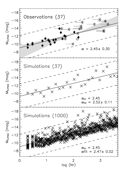
In the top panel of Fig. 16 we show the brightest cluster as a function of log()) from the sample of Larsen & Richtler (2000) with filled circles and Whitmore (2003) with open circles. The sample of Whitmore (2003) has been shifted to the right with 0.2 dex, which is the expected number of clusters missed between and based on a luminosity function with exponent . The in a certain magnitude interval relates to the slope of the LF as
| (7) |
where is the magnitude interval and is the slope of the LF. We have updated the data for NGC 1569, based on the data of Hunter et al. (2000). This was an outlying point in Whitmore (2003), but we found more clusters in Hunter et al. (2000).
We have over-plotted the expected increase in maximum cluster luminosity with assuming the luminosity function is a single power-law distribution and based on a range of exponent (), which is the observed range of slopes in this work. The fit to the closed circles is shown with the solid line, which falls nicely within the predicted area and corresponds to a exponent of the LF of . Note that although this value is slightly higher than found in § 4.2, it is still within the 1 error. Also we here use an indirect method to determine the slope of the LF, based on a small number of data points.
L02 has quantified the expected scatter in the maximum cluster luminosity. The 1 deviation is 1.04 mag from the mean and is independent of the number. We over-plotted the deviations. To show the effect of the expected scatter, we show a simulated set of maximum cluster luminosities as a function of in the middle and bottom panels of Fig. 16. The input exponent of the simulated LF was the value found from the fit to the observations (2.45). The same number of simulated maximum cluster luminosities as was observed is shown in the middle panel and a larger number in the bottom panel. The simulated luminosities show that luminosities close to the error line are expected even with the low number of galaxies. The 3 scatter is a little bit higher on the bright side of the fit, which is because of the power-law nature of the LF function.
For the galaxies studied here, we find that the luminosity of the brightest cluster can be accounted for by sampling statistics. This is in contrast with the most massive cluster. This can be understood by looking at Fig. 2 and Fig. 6. There we can see that the most luminous cluster in each galaxy is always a young cluster (log(age/yr) 7). The most massive cluster, however, is usually in the older bins, since these cover a larger time in which it is more likely to form a more massive clusters. The physical upper limits we have derived in this work are not reached when sampling a CIMF during 107 years.
7 Discussion
A truncation of the cluster mass function raises the question what physical mechanism could be responsible for this cut-off. An answer might be present in the mass spectrum of giant molecular clouds (GMCs). Williams & McKee (1997) have shown that there is a distinct cut-off at the high mass end of the mass function of GMCs in the Milky Way. There are no clouds observed above , while there are 100 GMCs expected above that cut-off, based on statistical arguments. This might be caused by shear effects which do not allow clouds to grow larger than a certain size. The size and the mass of clouds are directly related by the virial theorem. Assuming that star clusters are formed with a star formation efficiency of and that one single GMC produces one cluster, this implies it is not possible at this moment to form clusters more massive than in the Milky Way. The Milky Way has formed a few massive clusters in the last few Myr, like Westerlund 1 with a mass of (Clark et al. 2005) and the Arches and Quintuplet clusters in the Galactic center with masses of around (Figer et al. 1999).
A rough estimate can show that we would have expected more massive objects. Westerlund 1 is the most massive young cluster in the Milky Way disk. Of course we have to look at the size-of-sample that was used to discover it. Westerlund 1 is about 4.5 kpc away from the sun (Clark et al. 2005). Based on the most recent catalog of open clusters by Kharchenko et al. (2005), Lamers et al. (2005a) estimated the masses of clusters in the solar neighborhood. Within 600 pc from the sun, the catalog is complete until 200 , where about 100 clusters are found above that mass. The initial mass of the most massive cluster observed is estimated to be . The size of sample predicts . So within the solar neighborhood the mass of most massive cluster is determined by the size-of-sample effect. Assuming that the number density of clusters is constant until Westerlund 1, we can predict the expected maximum mass, based on statistical grounds. Based on the distance of 4.5 kpc, the expected number of clusters above 200 is about () times larger. This implies we would expect a maximum mass of . Although Westerlund 1 is a very massive cluster with , we would have expected at least one cluster above . Given that Westerlund 1 is highly obscured, it is unlikely that a 10 times more massive object would not have been found yet within a distance on 4.5 kpc from the sun. In fact, the mass of Westerlund 1 might be a reasonable upper limit, given that the most massive GMC is (Williams & McKee 1997) and a reasonable star formation efficiency of a few percent.
It is not clear what causes the cut-off of the cloud mass function. The maximum cluster mass seems to be environment dependent, since in the “Antennae” galaxies clusters of a few times are being formed. This could be because the maximum GMC mass is higher (Wilson et al. 2003), or because the star formation efficiency is much higher. The star formation efficiency is expected to be higher in high pressure environments (Elmegreen & Efremov 1997), which is the case in shock induced star formation environments like galaxy mergers (Schweizer 2005). The super massive cluster W3 in NGC 7252, with a dynamical mass of (Maraston et al. 2004), exceeds the limits we observe by almost two orders of magnitude. It was probably formed in the merger process of two gas-rich spirals and seems to be the tip of a continues power-law distribution (Miller et al. 1997).
As a comparison, the “Antennae” galaxies have not merged their nuclei yet. Simulations of the merging of two gas-rich spirals (Barnes & Hernquist 1991) have shown that in the third encounter the gas disks merge with relative velocities of more than 500 km s-1. Perhaps more massive clusters can be formed in these merging stages, due to the merging of clusters. Clusters also seem to form in complexes of multiple clusters and stars, with similar properties of their progenitor GMCs (Bastian et al. 2005a). Fellhauer & Kroupa (2005) have shown by numerical simulations that these complexes can collapse and form a single, diffuse, ultra-massive object, which might be the way W3 and other very massive clusters can be formed. During the merger shear-free regions exist, like in the overlap-region in the “Antennae”galaxies, where GMCs can grow bigger and more massive than in the galaxies we have studied here.
8 Conclusion
We have compared observed star cluster luminosity function in five galaxies with analytical cluster population models. Our main results can be summarized as follows:
-
•
there are no clusters in M51 more massive than , although they are predicted by the size-of-sample effect. When comparing the maximum cluster mass in increasing log(age/yr) bins, the LMC and SMC cluster population show an increase consistent with the size-of-sample of effect. The cluster population of M51, however, shows a much shallower increase. This suggests a physical upper limit to the masses of clusters M51, although the shallow increase can also be reproduced by a combined effect of cluster disruption, infant mortality and an increasing cluster formation rate.
-
•
when comparing the results of different function fits to the five galaxies in our sample, we find that the LF of the SMC, the LMC and NGC 5236 can be well approximated by a power-law (), with , while the LF of NGC 6946 and M51 are slightly better approximated with a double power-law or Schechter function.
-
•
when fitting a double power-law function to the LF of NGC 6946 we find a break point at = mag. Faint-ward of the bend a power-law with exponent can be fitted. Bright-ward of the bend an exponent of is found. The LF can also be well fitted by fit a Schechter function with a bend at = mag.
-
•
the LF of M51 shows a break at = mag. Faint-ward of the bend a power-law with exponent can be fitted. Bright-ward of the bend an exponent of is found. The LF of M51 is also well fitted by a Schechter function with a bend at = mag.
-
•
the cluster LFs can be reproduced with a synthetic cluster population model. The bend in the LF of NGC 6946, M51 and “Antennae” galaxies can be explained with a truncation of the cluster mass function at (M51/NGC 6946) and (“Antennae”).
In a follow-up study (Gieles et al. 2006b) we present an improved LF of star clusters in M51 based on HST/ACS data, taken as part of the Hubble Heritage project.
Acknowledgements.
We are very grateful to Deidre Hunter who kindly provided the data of the SMC and LMC clusters. We like to thank Carsten Weidner and Pavel Kroupa for useful discussion. We acknowledge research support from and hospitality at the International Space Science Institute (ISSI) in Berne (Switzerland), as part of an International Team programme. Finally, we thank an anonymous referee for very constructive comments on the manuscript, which have improved the paper.References
- Anders & Fritze-v. Alvensleben (2003) Anders, P. & Fritze-v. Alvensleben, U. 2003, A&A, 401, 1063
- Barnes & Hernquist (1991) Barnes, J. E. & Hernquist, L. E. 1991, ApJ, 370, L65
- Bastian et al. (2005a) Bastian, N., Gieles, M., Efremov, Y. N., & Lamers, H. J. G. L. M. 2005a, A&A, 443, 79
- Bastian et al. (2005b) Bastian, N., Gieles, M., Lamers, H. J. G. L. M., Scheepmaker, R. A., & de Grijs, R. 2005b, A&A, 431, 905
- Baumgardt & Makino (2003) Baumgardt, H. & Makino, J. 2003, MNRAS, 340, 227
- Bergvall et al. (2003) Bergvall, N., Laurikainen, E., & Aalto, S. 2003, A&A, 405, 31
- Bik et al. (2003) Bik, A., Lamers, H. J. G. L. M., Bastian, N., Panagia, N., & Romaniello, M. 2003, A&A, 397, 473
- Boutloukos & Lamers (2003) Boutloukos, S. G. & Lamers, H. J. G. L. M. 2003, MNRAS, 338, 717
- Clark et al. (2005) Clark, J. S., Negueruela, I., Crowther, P. A., & Goodwin, S. P. 2005, A&A, 434, 949
- de Grijs et al. (2003a) de Grijs, R., Anders, P., Bastian, N., et al. 2003a, MNRAS, 343, 1285
- de Grijs et al. (2003b) de Grijs, R., Fritze-v. Alvensleben, U., Anders, P., et al. 2003b, MNRAS, 342, 259
- Elmegreen & Efremov (1997) Elmegreen, B. G. & Efremov, Y. N. 1997, ApJ, 480, 235
- Fall (2004) Fall, S. M. 2004, in ASP Conf. Ser. 322: The Formation and Evolution of Massive Young Star Clusters, 399–+
- Feldmeier et al. (1997) Feldmeier, J. J., Ciardullo, R., & Jacoby, G. H. 1997, ApJ, 479, 231
- Fellhauer & Kroupa (2005) Fellhauer, M. & Kroupa, P. 2005, MNRAS, 359, 223
- Figer et al. (1999) Figer, D. F., Kim, S. S., Morris, M., et al. 1999, ApJ, 525, 750
- Fritze-v. Alvensleben (1999) Fritze-v. Alvensleben, U. 1999, A&A, 342, L25
- Gieles et al. (2005a) Gieles, M., Bastian, N., Lamers, H. J. G. L. M., & Mout, J. N. 2005, A&A, 441, 949
- Gieles et al. (2006b) Gieles, M., Larsen, S. S., Scheepmaker, R. A. et al. 2006, accepted for A&A Letters (astro-ph/0512298)
- Hunter et al. (2003) Hunter, D. A., Elmegreen, B. G., Dupuy, T. J., & Mortonson, M. 2003, AJ, 126, 1836
- Hunter et al. (2000) Hunter, D. A., O’Connell, R. W., Gallagher, J. S., & Smecker-Hane, T. A. 2000, AJ, 120, 2383
- Kharchenko et al. (2005) Kharchenko, N. V., Piskunov, A. E., Röser, S., Schilbach, E., & Scholz, R.-D. 2005, A&A, 438, 1163
- Kroupa & Boily (2002) Kroupa, P. & Boily, C. M. 2002, MNRAS, 336, 1188
- Lada & Lada (2003) Lada, C. J. & Lada, E. A. 2003, ARA&A, 41, 57
- Lamers et al. (2005a) Lamers, H. J. G. L. M., Gieles, M., Bastian, N., et al. 2005a, A&A, 441, 117
- Lamers et al. (2005b) Lamers, H. J. G. L. M., Gieles, M., & Portegies Zwart, S. F. 2005b, A&A, 429, 173
- Larsen (2000) Larsen, S. S. 2000, MNRAS, 319, 893
- Larsen (2002) Larsen, S. S. 2002, AJ, 124, 1393
- Larsen & Richtler (1999) Larsen, S. S. & Richtler, T. 1999, A&A, 345, 59
- Larsen & Richtler (2000) Larsen, S. S. & Richtler, T. 2000, A&A, 354, 836
- Leitherer et al. (1999) Leitherer, C., Schaerer, D., Goldader, J. D., et al. 1999, ApJS, 123, 3
- Maraston et al. (2004) Maraston, C., Bastian, N., Saglia, R. P., et al. 2004, A&A, 416, 467
- Massey (2002) Massey, P. 2002, ApJS, 141, 81
- Mengel et al. (2005) Mengel, S., Lehnert, M. D., Thatte, N., & Genzel, R. 2005, ArXiv Astrophysics e-prints
- Meurer et al. (1995) Meurer, G. R., Heckman, T. M., Leitherer, C., et al. 1995, AJ, 110, 2665
- Miller et al. (1997) Miller, B. W., Whitmore, B. C., Schweizer, F., & Fall, S. M. 1997, AJ, 114, 2381
- Salo & Laurikainen (2000) Salo, H. & Laurikainen, E. 2000, MNRAS, 319, 377
- Schechter (1976) Schechter, P. 1976, ApJ, 203, 297
- Schlegel et al. (1998) Schlegel, D. J., Finkbeiner, D. P., & Davis, M. 1998, ApJ, 500, 525
- Schulz et al. (2002) Schulz, J., Fritze-v. Alvensleben, U., Möller, C. S., & Fricke, K. J. 2002, A&A, 392, 1
- Schweizer (2005) Schweizer, F. 2005, in ASSL Vol. 329: Starbursts: From 30 Doradus to Lyman Break Galaxies, 143–+
- Solomon et al. (1987) Solomon, P. M., Rivolo, A. R., Barrett, J., & Yahil, A. 1987, ApJ, 319, 730
- Weidner et al. (2004) Weidner, C., Kroupa, P., & Larsen, S. S. 2004, MNRAS, 350, 1503
- Whitmore (2003) Whitmore, B. C. 2003, in A Decade of Hubble Space Telescope Science, 153–178
- Whitmore & Schweizer (1995) Whitmore, B. C. & Schweizer, F. 1995, AJ, 109, 960
- Whitmore et al. (1993) Whitmore, B. C., Schweizer, F., Leitherer, C., Borne, K., & Robert, C. 1993, AJ, 106, 1354
- Whitmore et al. (1999) Whitmore, B. C., Zhang, Q., Leitherer, C., et al. 1999, AJ, 118, 1551
- Williams & McKee (1997) Williams, J. P. & McKee, C. F. 1997, ApJ, 476, 166
- Wilson et al. (2003) Wilson, C. D., Scoville, N., Madden, S. C., & Charmandaris, V. 2003, ApJ, 599, 1049
- Zhang & Fall (1999) Zhang, Q. & Fall, S. M. 1999, ApJ, 527, L81