Fine structure in the phase space distribution of
nearby subdwarfs

We analysed the fine structure of the phase space distribution function of nearby subdwarfs using data extracted from various catalogues. Applying a new search strategy based on Dekker’s theory of galactic orbits, we found four overdensely populated regions in phase space. Three of them were correlated with previously known star streams: the Hyades–Pleiades and Hercules streams in the thin disk of the Milky Way and the Arcturus stream in the thick disk. In addition we find evidence for another stream in the thick disk, which resembles closely the Arcturus stream and probably has the same extragalactic origin.

1 Introduction

Fine structure in the velocity distribution of stars in the Milky Way was discovered and studied by O.J. Eggen during almost all of his career (Eggen 1996 and references therein). Some of Eggens’s star streams are associated with young open clusters and can be naturally interpreted as clouds of former members, now unbound and drifting away from the clusters. Other streams contain only stars older than 10 Gyrs. Since for many members distances were not known but had to be assumed in order to construct space velocities, the real existence of such old streams has often been doubted.

However, modern data seem to confirm the concept of old star streams. Helmi et al. (1999) found the signature of a cold stream in the velocity distribution of the halo stars of the Milky Way when analyzing Hipparcos data. This was confirmed later by Chiba & Beers (2000) using their own data (Beers et al. 2000). Helmi et al. (1999) interpreted this stream as part of the tidal debris of a disrupted satellite galaxy accreted by the Milky Way, which ended up in the halo. Indeed, numerical simulations have shown that relic stars from disrupted satellites can stay on orbits that are close together for many Gyrs (Helmi et al. 2003, Helmi 2004). These then show up as overdensities in phase space. In the same vein Navarro et al. (2004) argue that Eggens’s (1996) Arcturus group is another such debris stream, but in the thick disk of the Milky Way, dating back to an accretion event 5 to 8 Gyrs ago. These observations complement observations of ongoing satellite accretion such as of the Sagittarius dwarf galaxy (Ibata et al. 1994) or very recent accretion in the form of the Monoceros stream discovered in the outer disk of the Milky Way with SDSS data (Newberg et al. 2002, Yanny et al. 2003, Rocha–Pinto et al. 2003, Peñarrubia et al. 2005). Extended periods of the accretion of satellites onto massive galaxies are also theoretically expected. For instance, recent sophisticated simulations of the formation of a disk galaxy in the framework of cold dark matter cosmology and the cosmogony of galaxies by Abadi et al. (2003a, b) suggest that disrupted satellites significantly contribute not only to the stellar halo but also to the disk of a galaxy.

Old moving groups are also observed in the velocity distribution of thin disk stars in the solar neighbourhood. Using Hipparcos parallaxes and proper motions, Dehnen (1998) found new evidence of the Sirius–UMa, Pleiades–Hyades, and Hercules star streams by statistical methods. Even more convincingly these streams show up in the extensive data sample of the three–dimensional kinematical data of F and G stars in the solar neigbourhood by Nordström et al. (2004, hereafter NMA+). The crowding of these stars on orbits in certain parts of velocity space is attributed to dynamical effects. Dehnen (2000) and Fux (2001) demonstrate that the Hercules stream may well be due to an outer Lindblad resonance of the stars with the central bar of the Milky Way. The Sirius–UMa and Pleiades–Hyades streams, on the other hand, are probably due to orbital resonances of stars in the solar neighbourhood with spiral density waves in the Milky Way disk (De Simone et al. 2004, Quillen & Minchev 2005). However, there are also hints that further overdensities in velocity space might be relics of accreted satellites (Helmi et al. 2005).

Here we use our own data (Arifyanto et al. 2005; hereafter AFJW) on the kinematics of nearby subdwarfs and develop a new strategy to search for signatures of old star streams in the phase space distribution of the stars. We then cross check our findings with the NMA+ data.

2 Data and search strategy for streams

2.1 Data

AFJW construct their data set from the sample of F and G subdwarfs of Carney et al. (1994, hereafter CLLA), which is based on the Lowell Proper Motion Survey, the so–called Giclas stars. While keeping the precise radial velocity and metallicity data of CLLA, AFJW have significantly improved the accuracy of the distances and proper motions for a subset of the CLLA sample. The original CLLA sample contains 1464 stars, but kinematical and metallicity data are not available for every star. Many of the CLLA stars were observed with Hipparcos, and AFJW identified 483 stars in the astrometric TYC2+HIP catalogue (Wielen et al. 2001) and replaced the parallaxes and proper motions of CLLA by Hipparcos parallaxes and proper motions, respectively. The Hipparcos parallaxes were then used to recalibrate the photometric distance scale for the rest of the CLLA stars. AFJW could identify 259 CLLA stars in the Tycho–2 catalogue (Høg et al. 2000) and adopted the proper motions given there. Thus the sample of AFJW that forms the basis of our analysis contains 742 subdwarfs with greatly improved parallax and proper motion data. While the photometric distances were corrected by a factor of about 10%, the old NLTT proper motions were improved from an accuracy of 20 to 30 mas/yr to 2.5 mas/yr.

2.2 Search strategy

The aim of our search is to find overdensities of stars in phase space on orbits that stay close together. For that purpose we use Dekker’s (1976) theory of galactic orbits. Since the latter is not well known despite its usefulness, we repeat the basic steps here to estimate the parameters of stellar orbits. The first step is to separate the planar from the vertical motion of a star. This assumption is justified, because we are treating orbits of stars with disklike kinematics. Concentrating now on the planar motion in the galactic plane, the equation of motion of a star moving in the meridional plane is given by

$$\ddot{R}=-\frac{\partial\Phi_{\rm eff}}{\partial R}=-\frac{\partial}{\partial R}\left(\Phi(R)+\frac{1}{2}\frac{L^{2}}{R^{2}}\right)\,,$$ (1)

where $R$ denotes the galactocentric radius. The effective potential $\Phi_{\rm eff}$ is constructed in the usual way with both the gravitational potential $\Phi(R)$, which is assumed to be axisymmetric, and the vertical component of the angular momentum of the star $L$ . Dekker’s theory proceeds then like standard epicycle theory by choosing a mean guiding centre radius for the orbit of a star $R_{0}$ by setting

$$L=R_{0}^{2}\Omega(R_{0})\quad{\rm with}\quad\Omega(R)=\sqrt{\frac{1}{R}\frac{\partial\Phi}{\partial R}}$$ (2)

the mean angular frequency of a stellar orbit. The energy of a star on the circular mean guiding centre orbit is obviously given by

$$E_{0}=\Phi(R_{0})+\frac{1}{2}R_{0}^{2}\Omega^{2}(R_{0})\,.$$ (3)

Furthermore the epicyclic frequency $\kappa_{0}$ is introduced, $\kappa^{2}(R_{0})=4\Omega^{2}(R_{0})\big{[}1+\frac{1}{2}d\ln{\Omega}/d\ln{R}|_{\rm R_{0}}\big{]}$. The key point of Dekker’s (1976) formalism is to expand the potential with respect to $\frac{1}{R}$ around $\frac{1}{R_{0}}$ as

$$\Phi(R) = \Phi(R_{0})+\frac{d\Phi}{d(\frac{1}{R})}\bigg{|}_{\rm R_{0}}\left(\frac{1}{R}-\frac{1}{R_{0}}\right)$$

$$+ \frac{1}{2}\frac{d^{2}\Phi}{d(\frac{1}{R})^{2}}\bigg{|}_{\rm R_{0}}\left(\frac{1}{R}-\frac{1}{R_{0}}\right)^{2}\,,$$

which is asymmetric with respect to $R_{0}$ and thus more realistic than the Taylor expansion of $\Phi(R)$ in the standard epicycle theory. Expression (4) is written as

$$\Phi(R)=a_{0}-\frac{b_{0}}{R}+\frac{c}{R^{2}}$$ (5)

with the coefficients $a_{0}=E_{0}+\frac{1}{2}R_{0}^{2}\kappa_{0}^{2}$, $b_{0}=R_{0}^{3}\kappa_{0}^{2}$, and $c_{0}=\frac{1}{2}R_{0}^{4}(\kappa_{0}^{2}-\Omega_{0}^{2})$. The turning points of the radial motion of a star $R_{\rm t}$ are defined by the condition $E=\Phi_{\rm eff}(R_{\rm t})$. If the potential (5) is inserted, this leads to

$$\frac{R_{\rm t}}{R_{0}}=\frac{1}{1\pm e}\quad{\rm with}\quad e=\sqrt{\frac{2(E-E_{0})}{R_{0}^{2}\kappa_{0}^{2}}}\,.$$ (6)

The orbits are thus characterised by the two isolating integrals of motion angular momentum $L$ and energy $E$. By comparing her approximation (4) with various forms of exact potentials Dekker (1976) has shown that it gives reliable results up to eccentricities of $e\approx 0.5$. $L$ and $e$ can be estimated directly for each star in our sample. We assume that every star is essentially at the position of the Sun and find

$$L=R_{\odot}(V+V_{\rm LSR})=R_{0}V_{\rm LSR}\,.$$ (7)

Here $R_{\odot}$ denotes the galactocentric distance of the Sun, for which we adopt 8 kpc, $V$ is the velocity component of the star pointing into the direction of galactic rotation, and $V_{\rm LSR}$ is the circular velocity of the local standard of rest, for which we adopt 220 km/s. The eccentricity $e$ is given by

$$e_{R_{0}}=\sqrt{\frac{U^{2}+\frac{\kappa_{0}^{2}}{\Omega_{0}^{2}}V^{2}}{R_{0}^{2}\kappa_{0}^{2}}}\,,$$ (8)

with $U=-\dot{R}$ the radial velocity component of the star. In the following we assume a flat rotation curve implying $\kappa_{0}^{2}/\Omega_{0}^{2}=2$ and $R_{0}^{2}\kappa_{0}^{2}=2\,V_{\rm LSR}^{2}$. The search for overdensities in phase space of stars on essentially the same orbits is carried out in practice in a space spanned up by $\sqrt{U^{2}+2\,V^{2}}$ and $V$. In addition we study the distribution of stars in our sample in ($|W|$, $V$) velocity space. Since the Sun is located very close to the galactic midplane, the absolute value of the vertical velocity component$|W|$ is a measure of the energy associated with the vertical motion of a star.

3 Results and discussion

We split our sample up into two subsets with metallicities of [Fe/H] $>$ -0.6 and [Fe/H] $\leq$ -0.6, respectively.

3.1 Thin disk

The stars in our sample with metallicities [Fe/H] $>$ -0.6 dex have kinematics of the old thin disk of the Milky Way. Of course the metallicity cut is somewhat arbitrary, because the thin and thick disk populations do not have a bimodal metallicity distribution, but the transition is quite gradual. In Fig. 1 we show the distribution of 309 stars, which have $|W|$ velocities $<$ 50 km/s, over $\sqrt{U^{2}+2\,V^{2}}$ versus $V$ and $|W|$ versus $V$, respectively. The space velocities have been reduced to the local standard of rest by adding the solar motion $(U,V,W)_{\odot}=(10.0,5.2,7.2)$ km/s (Dehnen & Binney 1998) to the observed space velocities. Instead of scatter plots we show colour coded wavelet transforms of our data in Fig. 1. For this purpose we used the two–dimensional Mexican–hat wavelet transform described by Skuljan et al. (1999). After some experimentation we found that a wavelet scale of 10 km/s showed the overdensities in the data samples in the clearest way. The Hercules stream at $V\approx$ -40 km/s is clearly visible as is, to a lesser degree, the Hyades–Pleiades stream at $V\approx$ -15 km/s, and in both cases exactly where expected (Dehnen 2000, NMA+). Since these streams have been discussed widely in the literature, we do not go into any further details. We present them mainly to demonstrate that by recovering previously known streams our method is well–suited to searching for cold star streams.

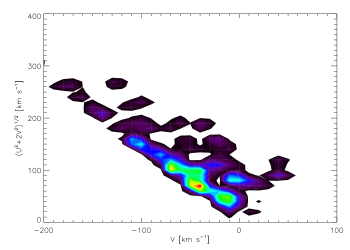
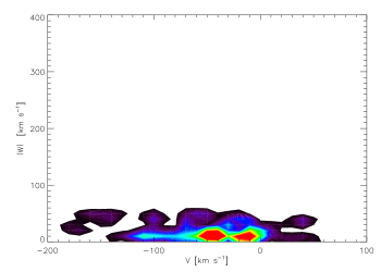
Figure 1: Wavelet analysis of the distribution of thin disk stars over $\sqrt{U^{2}+2\,V^{2}}$ versus $V$ (top panel) and over $|W|$ versus $V$ (bottom panel). The wavelet scale of the Mexican hat kernel is 10 km/s and a linear colour table from black over lilac, green, yellow to red is adopted.

On the other hand, it is instructive in order to assess the reality of such overdensities in phase space to compare the observed distribution with Monte Carlo simulations of realisations of a smooth distribution. In Fig. 2 we show such a Monte Carlo simulation analysed in the same way as the observations. Three hundred nine stars were distributed in the range -200 km/s $<$ $V$ $<$ 50 km/s and $\sqrt{U^{2}+2\,V^{2}}$ $<$ 300 km/s, respectively, according to a Schwarzschild distribution

$$f\propto\exp{-\frac{1}{2}\left[\left(\frac{U}{\sigma_{\rm U}}\right)^{2}+\left(\frac{V-\bar{V}}{\sigma_{\rm V}}\right)^{2}\right]}\,,$$ (9)

with parameters $\sigma_{\rm U}$ = 45 km/s, $\sigma_{\rm V}$ = 32 km/s, and $\bar{V}$ = 26 km/s, which have been derived from the CNS4 catalogue as representative of disk stars in the solar neighbourhood (Jahreiß & Wielen 1997). As can be seen from Fig. 2 the simulated distributions looks generally smoother than the observed distribution but also show considerable Poisson fluctuations that can be confused with real cold star streams. The only remedy for detecting real star streams is obviously to search for such streams in separate data sets.

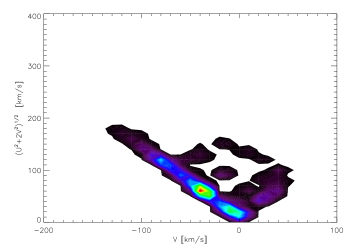
Figure 2: Same as Fig. 1, but for 309 stars distributed randomly in phase space according to a smooth Schwarzschild distribution

3.2 Thick disk

The remaining stars of our sample with metallicities [Fe/H] $\leq$ -0.6 dex belong to the thick disk and halo of the Milky Way. The distribution of 382 stars is shown in Fig. 3 in the same way as above, but now restricted to $|W|$ $<$ 100 km/s. There are two distinct features in the phase–space distribution function. The lesser feature at $V\approx$ -125 km/s corresponds to the familiar Arcturus stream (Eggen 1996, Navarro et al. 2004). The stars in this phase space region are listed in Table 1 (available only in electronic form) giving all relevant data. The kinematics and metallicities of the stars listed in Table 1 can be compared with those of the stars considered by Navarro et al. (2004; their Figs. 2 and 3) as members of the Arcturus group. Actually there is one common star, G2-34. The kinematics and metallicities agree so well with each other that, even though the reality of low number overdensities is difficult to assess, we are confident that both investigations have identified the same stream. Arcturus itself, although not a CLLA star, lies in Fig. 3 at $V$ = -114 km/s, $\sqrt{U^{2}+2\,V^{2}}$ = 165 km/s, and $|W|$ = 4 km/s, respectively. With a metallicity of [Fe/H] = -0.55 (Luck & Heiter 2005), it fits well to the rest of the presumed stream members. We place the centre of the stream at $V$ = -125 km/s and $\sqrt{U^{2}+2V^{2}}$ = 185 km/s implying $|U|$ = 55 km/s. According to Eq. (7) the guiding centre radius of the orbits of the stars now passing close to the Sun is $R_{0}=0.43\,R_{\odot}$ = 3.5 kpc. The eccentricity is $e_{R_{0}}$ = 0.59 implying an outer turning radius of $R_{t}=2.5\,R_{0}$ = 8.5 kpc. The stars are apparently close to apogalacticon, when they are at their slowest on their orbits and the detection probability is highest. In Fig. 4 we show a colour–magnitude diagram of the presumed members of the Arcturus stream listed in Table 1. Overlaid are theoretical isochrones of subdwarfs with an age of 12 Gyrs calculated for metallicities [Fe/H] = -0.5, -1, and -1.5, respectively (Yi et al. 2001). The good fit of the isochrones indicates that the selected stars must be very old. In particular the tip of the main sequence fits well to the turn–off points of the isochrones. This is not a selection effect in the AFJW sample, because the brightest stars in the sample have absolute magnitudes of $M_{\rm V}$ $<$ 4 mag. Judging from the ages and metallicities of the stars and the similarity of their kinematics with that of debris from a disrupted satellite in the vicinity of the Sun, we follow Navarro et al. (2004) in concluding that the members of the Arcturus stream are of extragalactic origin.

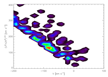
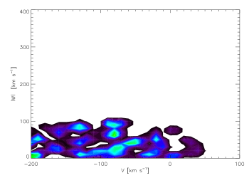
Figure 3: Same as Fig. 1, but for thick disk stars.

Figure 4: Colour–magnitude diagrams of the presumed members of the Arcturus stream (left panel) and the proposed new stream (right panel). Overlaid are theoretical isochrones for subdwarfs with an age of 12 Gyrs and and metallicities of [Fe/H] = -0.5, -1, and -1.5 (from right to left).

As can be seen in Fig. 3 there is a second strong feature in the phase–space distribution of the thick–disk stars. This seems to be even more significant than the overdensity in the Arcturus region. The stars in this overdensely populated region are listed in Table 2. To our knowledge the existence of a cold star stream in this part of phase space has not been suggested before. Comparing Figs. 3 and 1 we find a clear indication of a corresponding density enhancement at $V$ $\approx$ -70 km/s in Fig. 1. This phase–space feature can thus also be traced among the more–metal rich stars, but is more prominently seen in the metal–poor population.

In order to test the robustness of our findings we analysed the Copenhagen–Geneva Survey of nearby F and G stars (NMA+). This is based on Hipparcos parallaxes, Tycho–2 proper motions, radial velocities, and Strömgren photometry measured by the authors themselves. We have drawn all those stars from the catalogue with metallicities [Fe/H] $<$ -0.6 and show a wavelet analysis of the phase–space distribution function of 591 stars in Fig. 5 in the same way as in Figs. 1 and 3.

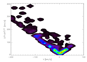
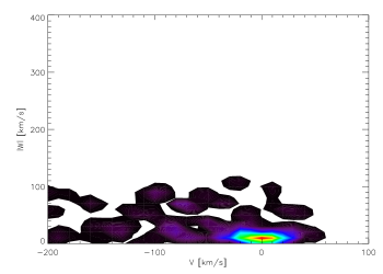
Figure 5: Same as Fig. 1, but for stars drawn from the Nordström et al. (2004) sample with metallicities [Fe/H] $<$ -0.6.

Comparing Figs. 5 and 3 it becomes immediately clear that the NMA+ sample is much more fully populated at low space velocities. This reflects that the latter is kinematically unbiased, whereas the CLLA sample is biased towards high proper motion stars. Eggen’s classical moving groups show up very clearly: the Sirius–UMa group at positive $V$ velocities, the Pleiades–Hyades stream at $V$ $\approx$ -20 km/s, and the Hercules stream at $V$ $\approx$ -40 km/s.

Even though these moving groups were originally devised by Eggen among thin disk stars with metallicities of [Fe/H] $\approx$ 0, they are also very prominent among the metal–poor stars. This indicates that the origins of the moving groups cannot be dissolving open clusters, but must be due to non–axisymmetric perturbations of the gravitational potential of the Milky Way (Dehnen 2000, Quillen & Minchev 2005). In Fig. 5 there is a weak but significant sign of the Arcturus stream, and some of the stars found as members of the Arcturus stream in the AFJW sample appear in the NMA+ catalogue. In our view this is due to the kinematical bias in the AFJW sample, so that the phase space is more richly populated at these negative $V$–velocities than in the NMA+ sample. For instance, in the NMA+ sample there are 144 stars with -200 km/s $<$ $V$ $<$ -50 km/s and $\sqrt{U^{2}+2\,V^{2}}$ $<$ 400 km/s, respectively, whereas in the AFJW sample there are 191 stars in the same range. However, the overdensity between -100 km/s $<$ $V$ $<$ -60 km/s is clearly discernible in Fig. 5, which confirms the detection of the new cold star stream claimed above.

Our data as given in Tables 1 and 2 show that the velocity and metallicity distributions of the members of the proposed new stream and the Arcturus stream are practically identical. Also the colour–magnitude diagrams shown in Fig. 4 seem to indicate that the stars stem from the same population. We place the centre of the proposed new stream at $V$ = -80 km/s and $\sqrt{U^{2}+2V^{2}}$ = 130 km/s implying $|U|$ = 64 km/s. The mean guiding centre radius of the orbits of these stars now passing close to the sun is $R_{0}=0.64\,R_{\odot}$ = 5.1 kpc. The eccentricity is $e_{R_{0}}$ = 0.42 and the outer turning radius is at $R_{\rm t}=1.7\,R_{0}$ = 8.7 kpc. Thus the stars of the proposed new stream are also on their orbits close to apogalacticon.

Their orbits are actually very similar to the orbits of the presumed members of the Arcturus stream. We can at present only speculate about the possible origin of the stream. However, the similarity of the characteristics of the new stream with the Arcturus stream seems to point to an extragalactic origin. Moreover, both streams are probably related to each other. Indeed, Helmi et al. (2005) show that in numerical simulations of the disruption of a satellite galaxy falling into its parent galaxy, the satellite debris can end up in several cold star streams with roughly the same characteristic eccentricities of their orbits. Precisely this seems to be the case here, so that both streams can have very well originated from the same accretion event of a dwarf galaxy into the Milky Way. How the star streams discussed here are related to the star streams reported by Helmi et al. (2005), especially their groups 2 and 3, has yet to be explored.

Table 1: Potential members of the Arcturus stream

Name RA[2000] Dec[2000] $$V$$ Plx

Hip/Giclas deg deg mag mas mas/yr mas/yr mas/yr mas/yr mas/yr

13111 42.15594864 22.59843445 10.10 11.03 55.03 -359.47 1.55 1.07 0.97

36491 112.62090302 18.96128273 8.48 20.00 27.80 -436.75 1.45 0.95 0.62

36710 113.26815033 76.92041016 10.32 12.93 242.95 -201.59 1.42 0.96 1.28

40613 124.37228394 -3.98961496 7.74 20.46 -145.25 -438.59 1.12 0.88 0.91

53070 162.86718750 20.27749062 8.21 19.23 -260.72 -456.01 1.11 0.71 0.62

58253 179.20997620 13.37740707 9.95 11.98 -320.47 -173.65 1.49 0.90 0.73

74033 226.94375610 8.87977409 8.26 15.40 -518.44 -57.96 1.33 0.86 0.86

94931 289.75228882 41.63460541 8.87 28.28 98.78 -631.15 0.85 0.72 0.70

105888 321.67877197 5.44163942 8.49 13.02 167.04 -246.55 1.09 0.95 0.65

113514 344.83105469 12.19233322 8.35 20.59 332.17 -156.65 1.14 0.90 0.83

77637 237.74555969 8.42326450 9.95 10.07 -234.80 -159.80 1.39 1.47 1.51

G72-12 23.03840446 34.55577087 10.82 9.30 161.10 -223.20 1.37 1.80 1.80

G4-2 32.83348846 9.62153053 10.68 9.95 142.40 -267.70 1.47 2.50 2.30

G102-44 90.68071747 13.07698059 10.84 7.78 232.20 -148.30 1.15 1.50 1.50

G101-25 93.26070404 38.91038132 10.79 9.00 132.20 -199.60 1.33 3.60 3.40

G103-53 100.94363403 25.52507973 10.19 10.31 -7.60 -314.30 1.52 2.00 2.10

G42-34 150.80117798 19.84084129 10.70 13.16 -82.50 -343.60 1.95 1.50 1.60

G139-49 264.20046997 2.83879447 10.70 10.43 -137.80 -190.30 1.27 1.30 1.30

G204-30 267.49429321 37.52183914 10.27 9.72 -215.20 -165.50 1.44 3.20 3.00

G26-1 321.69931030 -8.39890003 11.27 6.34 56.70 -221.60 0.73 2.30 2.50

G265-43W 325.39273071 85.91363525 10.52 13.80 239.80 108.50 2.04 2.80 3.00

G241-7 336.42810059 69.52659607 10.50 9.10 172.80 91.50 1.34 1.80 1.90

Name B-V RV [Fe/H] U V W

Hip/Giclas mag km/s km/s dex km/s km/s km/s

13111 0.580 -22.3 0.7 -1.00 34.87 -125.83 -88.74

36491 0.538 90.9 0.8 -0.81 -58.52 -124.68 -7.35

36710 0.722 -71.3 0.6 -0.60 33.97 -122.70 47.65

40613 0.584 113.0 0.4 -0.51 -38.74 -144.44 -43.19

53070 0.498 65.4 0.8 -1.56 -35.44 -140.24 10.98

58253 0.700 28.9 0.6 -0.51 -80.23 -122.25 -16.00

74033 0.575 -60.6 0.7 -0.89 -114.20 -125.63 25.19

94931 0.806 -121.1 0.6 -0.87 55.68 -125.58 -85.21

105888 0.572 -84.6 0.6 -0.80 -33.54 -125.79 -44.34

113514 0.580 -122.8 0.5 -0.67 -55.13 -135.58 28.43

77637 0.591 -51.6 1.0 -1.15 -37.11 -138.26 6.81

G72-12 0.830 -33.8 0.8 -0.25 -23.01 -123.70 -70.70

G4-2 0.740 38.3 0.3 -0.80 -20.31 -122.47 -83.21

G102-44 0.710 -28.8 0.5 -0.62 61.06 -136.59 81.41

G105-25 0.820 -47.6 0.4 -0.14 36.30 -129.67 5.87

G103-53 0.680 9.2 0.8 -0.70 0.39 -130.49 -62.86

G42-34 0.850 37.5 0.8 -0.81 -2.93 -131.93 -13.93

G139-49 0.670 -95.7 0.7 -1.23 -37.19 -137.70 -14.74

G204-30 0.600 -70.7 0.6 -0.98 48.82 -136.30 39.61

G26-1 0.490 14.5 0.9 -1.87 46.28 -131.91 -99.60

G265-43W 0.800 -131.7 0.4 -0.76 -19.61 -134.02 -84.70

G241-7 0.620 -114.2 0.7 -0.97 -53.98 -140.39 -28.18

Table 2: Potential members of the proposed new stream

Name RA[2000] Dec[2000] $$V$$ Plx

Hip/Giclas deg deg mag mas mas/yr mas/yr mas/yr mas/yr mas/yr

9080 29.23373795 11.66352558 10.52 13.26 378.47 2.28 1.97 1.38 1.38

10652 34.27974319 21.56681061 9.06 14.43 473.77 83.43 1.29 0.77 0.69

11952 38.54603577 -12.38429260 9.77 8.67 60.47 -185.07 1.78 1.21 1.24

16169 52.08785248 -6.53092098 8.23 21.98 358.02 -195.35 1.13 1.00 0.76

17147 55.09193802 -3.21697974 6.68 41.07 690.50 -213.58 0.85 0.86 0.79

22020 71.01499176 52.98161697 9.10 10.76 64.35 -294.97 1.38 1.04 1.00

22777 73.48664093 69.23905945 9.78 13.44 219.93 -124.84 1.54 0.92 1.11

24030 77.48732758 5.55742788 9.71 10.29 269.99 -71.18 1.64 1.26 0.97

26452 84.41486359 68.73518372 9.60 13.14 245.55 -143.16 1.54 0.94 1.04

29814 94.17899323 47.06034470 9.18 20.39 57.31 -493.15 1.30 0.96 0.69

31740 99.60284424 48.79860687 10.11 11.92 131.60 -258.21 1.66 1.41 1.21

34642 107.62411499 53.25177765 8.80 10.77 -73.41 -241.43 1.21 1.02 0.83

50965 156.14868164 -5.51967478 9.80 9.70 -242.50 -166.16 1.40 1.05 1.00

61974 190.50057983 72.96403503 9.25 15.38 -287.50 -67.43 0.94 0.89 0.86

62607 192.43678284 1.18803751 8.13 30.12 -79.55 -644.49 0.91 0.61 0.48

73773 226.19566345 64.81214142 9.46 17.81 -255.17 -14.04 0.88 0.75 0.82

77122 236.21554565 62.86030579 8.95 11.53 -254.97 129.00 0.78 0.81 0.91

80700 247.14978027 3.25295258 8.81 21.50 -12.87 -526.94 1.27 0.93 0.88

89144 272.90850830 32.17737198 11.10 9.40 -96.72 -207.54 1.82 1.68 1.73

90365 276.59140015 8.61576462 8.32 26.30 -195.91 -468.58 1.05 0.88 0.75

92918 283.97070312 -5.74521637 7.46 29.77 -200.21 -388.80 1.04 0.89 0.73

102923 312.77783203 7.02700377 9.82 20.71 237.77 -361.96 1.62 1.41 0.84

104913 318.77395630 62.84111404 9.56 14.51 122.87 260.66 0.89 0.87 0.89

112811 342.69140625 1.86516070 9.33 16.66 100.35 -384.38 1.33 0.97 0.84

114661 348.41174316 39.41738892 11.02 14.09 173.67 -313.88 2.18 1.63 1.28

115359 350.49285889 16.63253784 8.92 14.97 406.56 -49.04 1.22 0.93 0.86

118115 359.38964844 -9.64751911 7.89 20.98 454.84 -146.12 1.20 0.97 0.58

G30-46 2.05598330 15.00853062 11.01 8.91 220.70 -51.20 1.32 1.70 1.60

G69-21 11.66600418 33.82573700 10.34 9.20 250.20 -23.20 1.36 1.50 1.60

G71-33 26.30754089 3.51369452 10.63 8.91 224.10 -12.10 1.03 1.20 1.20

G5-44 53.57446671 22.98726463 9.18 10.83 150.70 -169.00 1.60 0.90 0.90

G78-41 53.73811722 38.30670166 10.21 9.83 144.10 -144.20 1.45 2.50 2.50

G99-40 88.23098755 -3.49025011 9.19 10.97 268.80 -49.80 1.62 1.20 1.10

G192-21 92.50205231 50.15151215 8.52 17.11 205.80 -265.70 2.53 1.20 1.30

G110-38 106.72556305 18.13643265 11.34 9.40 9.10 -167.70 1.39 1.70 1.70

G146-76 164.98948669 44.77882004 10.49 15.28 -101.80 -219.80 1.77 1.30 1.30

G10-12 169.80845642 5.67945290 9.29 25.16 -307.60 -74.20 3.72 1.40 1.40

G197-45 182.37043762 51.93362045 10.73 10.97 -235.30 -114.30 1.62 2.30 2.20

G66-51 225.20860291 2.12708616 10.63 11.11 -177.50 -109.30 1.36 1.40 1.40

G230-45 310.06958008 54.21994019 11.43 9.72 83.40 224.70 1.44 3.00 2.70

G25-5 312.33590698 1.92505836 10.11 10.31 -43.60 -189.20 1.52 1.30 1.30

G26-8 322.93942261 -1.92733061 10.47 11.41 203.00 -68.60 1.69 1.70 1.70

G28-16 341.91043091 6.42221117 11.59 7.99 250.60 -77.40 1.18 2.70 2.70

G67-40 345.44311523 11.82143307 10.66 9.50 286.70 -79.40 1.41 1.70 1.60

Table 2: cont.

Name B-V RV $$\sigma_{\rm RV}$$ [Fe/H] U V W

Hip/Giclas mag km/s km/s dex km/s km/s km/s

9080 0.785 -10.7 0.9 -0.39 -93.51 -88.77 42.41

10652 0.621 -21.1 0.9 -0.89 -99.83 -92.30 83.28

11952 0.437 24.0 0.7 -1.82 27.76 -99.19 -36.06

16169 0.619 63.5 0.5 -0.58 -56.55 -90.59 -19.11

17147 0.554 120.3 0.6 -0.85 -109.88 -85.71 -44.86

22020 0.667 30.2 0.3 0.20 -82.86 -89.87 -60.51

22777 0.850 -45.6 0.5 -0.42 -7.82 -97.26 22.69

24030 0.520 -16.0 0.8 -0.92 10.42 -93.38 89.29

26452 0.513 -35.6 0.7 -0.89 -7.89 -100.11 41.20

29814 0.769 22.6 0.4 -0.55 -54.64 -99.83 -29.69

31740 0.730 85.9 0.4 -0.61 -101.93 -93.82 38.36

34642 0.600 -28.6 0.6 -0.73 -23.64 -92.83 -63.07

50965 0.580 20.6 0.6 -0.63 -61.88 -93.89 -91.75

61974 0.615 -43.2 0.7 -0.86 -50.36 -85.29 -18.44

62607 0.686 2.4 1.0 -0.81 39.48 -84.29 -42.29

73773 0.814 -69.5 0.4 0.00 -24.27 -92.86 -15.66

77122 0.580 -48.8 7.2 -0.87 -88.72 -90.59 10.33

80700 0.770 25.2 0.7 -0.17 80.96 -80.32 -33.70

89144 0.780 -38.0 0.8 -0.49 78.92 -92.41 -3.24

90365 0.764 -18.1 0.4 -0.15 42.89 -82.43 -8.58

92918 0.747 -73.4 0.3 -0.03 -31.25 -96.10 5.00

102923 0.900 -61.8 0.6 -0.07 -21.53 -97.77 -60.20

104913 0.751 -64.6 0.6 -0.27 -74.40 -84.82 17.53

112811 0.683 -4.1 0.8 -0.81 28.97 -89.88 -62.26

114661 0.689 -56.3 1.2 -2.68 9.71 -93.73 -94.11

115359 0.610 -40.4 0.5 -0.63 -101.86 -85.55 -27.46

118115 0.643 -31.2 0.5 -0.02 -74.78 -83.84 -2.35

G30-46 0.890 -22.6 0.6 0.20 -84.69 -86.10 -21.34

G69-21 0.680 -15.7 0.8 -0.57 -97.53 -86.43 -5.22

G71-33 0.480 -9.6 1.5 -2.33 -82.74 -81.47 29.43

G5-44 0.610 25.4 0.5 -0.06 -41.36 -90.59 -23.50

G78-41 0.670 -10.7 0.6 -0.65 -28.33 -94.13 -10.79

G99-40 0.560 49.6 0.6 -0.45 -27.56 -97.82 78.02

G192-21 0.560 -18.6 0.6 -0.64 -3.60 -93.73 14.76

G110-38 0.790 65.5 0.5 -0.67 -42.64 -96.55 -17.96

G146-76 0.670 -115.2 0.7 -2.31 41.50 -86.27 -98.76

G10-12 0.810 133.0 0.7 -0.92 -63.69 -96.28 88.98

G197-45 0.720 23.4 0.6 -0.92 -77.58 -81.84 24.70

G66-51 0.710 -118.8 0.4 -1.09 -96.02 -84.60 -75.15

G230-45 0.800 -79.8 0.7 -0.87 -109.04 -87.34 22.67

G25-5 0.670 -37.9 0.6 -0.66 34.72 -90.07 -9.38

G26-8 0.850 -83.1 0.7 -0.32 -89.16 -80.25 -21.01

G28-16 0.810 -25.0 0.5 -0.86 -105.96 -89.29 -75.09

G67-40 0.750 -29.3 0.4 -0.64 -103.86 -90.36 -62.80