Constraining the Cosmological Parameters and Transition Redshift with Gamma-Ray Bursts and Supernovae

Abstract

A new method of measuring cosmology with gamma-ray bursts(GRBs) has been proposed by Liang and Zhang recently. In this method, only observable quantities including the rest frame peak energy of the $\nu F_{\nu}$ spectrum $(E_{p}^{{}^{\prime}})$, the isotropic energy of GRB $(E_{\gamma,iso})$, and the break time of the optical afterglow light curves in the rest frame $(t_{b}^{{}^{\prime}})$ are used. By considering this method we constrain the cosmological parameters and the redshift at which the universe expanded from the deceleration to acceleration phase. We add five recently-detected GRBs to the sample and derive $E_{\gamma,{\rm{iso}}}/10^{52}{\rm ergs}=(0.93\pm 0.25)\times(E^{{}^{\prime}}_{\rm{p}}/{\rm 100\ keV})^{1.91\pm 0.32}\times(t^{{}^{\prime}}_{\rm{b}}/1{\rm day})^{-0.93\pm 0.38}$ for a flat universe with $\Omega_{M}=0.28$ and $H_{0}=71.0$ km s^-1 Mpc^-1. This relation is independent of the medium density around bursts and the efficiency of conversion of the explosion energy to gamma-ray energy. We regard the $E_{\gamma,{\rm{iso}}}(E_{\rm{p}}^{{}^{\prime}},t_{\rm{b}}^{{}^{\prime}}$) relationship as a standard candle and find $0.05<\Omega_{\rm{M}}<0.48$ and $\Omega_{\Lambda}<1.15$ (at the $1\sigma$ confidence level). In a flat universe with the cosmological constant we obtain $0.25<\Omega_{\rm{M}}<0.46$ and $0.54<\Omega_{\Lambda}<0.78$ at the $1\sigma$ confidence level. The transition redshift is $z_{T}=0.69_{-0.12}^{+0.11}$. Combining 20 GRBs with 157 type Ia supernovae, we find $\Omega_{M}=0.29\pm 0.03$ for a flat universe and the transition redshift is $z_{T}=0.61_{-0.05}^{+0.06}$, which is slightly larger than the value found by considering SNe Ia alone. In particular, We also discuss several dark-energy models in which the equation of state $w(z)$ is parameterized, and investigate constraints on the cosmological parameters in detail.

1 Introduction

The property of dark energy and the physical cause of acceleration of the present universe are two of the most difficult problems in modern cosmology. In past several years, many authors used distant type Ia supernovae (SNe Ia) (Riess et al. 1998; Perlmutter et al. 1999; Riess et al. 2004), cosmic microwave background (CMB) fluctuations (Bennett et al. 2003; Spergel et al. 2003), and large-scale structure (LSS) (Tegmark et al. 2004) to explore cosmology. Very recently, there have been extensive discussions on using gamma-ray bursts (GRBs) to constrain cosmological constraints (Dai et al. 2004; Ghirlanda et al. 2004; Xu et al. 2005; Firmani et al. 2005; Friedman & Bloom 2005; Mortsell & Sollerman 2005; Di Girolamo et al. 2005; Liang & Zhang 2005; Lamb et al. 2005).

SNe Ia have been considered as astronomical standard candles and used to measure the geometry and dynamics of the universe. Phillips (1993) found the intrinsic relation in SNe Ia: $L_{p}=a\times\bigtriangleup{m}_{15}^{b}$, where $L_{p}$ is the peak luminosity and $\bigtriangleup{m}_{15}$ is the decline rate in the optical band at day 15 after the peak. This relation and other similar relations can be used to explore cosmology. Riess et al (1998) considered 16 high-redshift supernovae and 34 nearby supernovae and found that our present universe has been accelerating. Perlmutter et al (1999) used 42 SNe Ia and drew the same conclusion. Riess et al (2004) selected 157 well-measured SNe Ia, which is called the“gold” sample. Assuming a flat universe, they concluded that: (1) Using the strong prior of $\Omega_{M}=0.27\pm 0.04$, fitting a static dark energy equation of state yields $-1.46<w<-0.78$ (95%C.L.). (2) Assuming a possible redshift dependence of $w(z)$ (using $w(z)=w_{0}+w_{1}z$), the data with the strong prior indicate that the region $w_{1}<0$ and especially the quadrant ($w_{0}>-1$ and $w_{1}<0$) are the least favored. (3) Expand $q(z)$ into two terms: $q(z)=q_{0}+zdq/dz$. If the transition redshift is defined through $q(z_{T})=0$, they found $z_{T}=0.46\pm 0.13$. The cosmological use of SNe Ia has the following advantages: the SN Ia sample is very large and includes low-$z$ sources, so the parameters $a$ and $b$ can be calibrated by using low-$z$ SNe Ia. The Phillips relation and other similar relations are intrinsic and cosmology-independent so that they can be used to explore cosmology. But they also have disadvantages: the interstellar medium extinction may exist when optical photons propagate towards us. In addition, the maximum redshift of SNe Ia is only about 1.7 and thus the earlier universe may not be well-studied. Higher-redshift SNe Ia are necessary to eliminate parameter degeneracies in studying the evolution of dark energy (Weller & Albrencht 2002; Linder & Huterer 2003).

GRBs are the most intense electromagnetic explosions in the universe after the big bang. They have been well understood since the discovery of afterglows in 1997 (for review articles see Piran 1999, 2004; van Paradijs et al. 2000; Mészáros 2002; Zhang & Mészáros 2004). It has been widely believed that they should be detectable out to very high redshifts (Lamb & Reichart 2000; Ciardi & Loeb 2000; Bromm & Loeb 2002; Gou et al. 2004). Schaefer (2003) derived the luminosity distances of 9 GRBs with known redshifts by using two quantities (the spectral lag and the variability). He obtained the first GRB Hubble diagram with the mass density $\Omega_{M}<0.35$ (at the $1\sigma$ confidence level). Ghirlanda et al. (2004a) found the relation between isotropic-equivalent energy $E_{\gamma,iso}$ and the local-observer peak energy $E_{p}^{{}^{\prime}}$ (i.e., the Ghirlanda relation). Unfortunately, because of the absence of low-$z$ GRBs, the Ghirlanda relation has been obtained only from moderate-$z$ GRBs. So this relation is cosmology-dependent. Dai, Liang & Xu (2004) used for the first time the Ghirlanda relation with 12 bursts and found the mass density $\Omega_{M}=0.35\pm 0.15$ (at the $1\sigma$ confidence level) for a flat universe with the cosmological constant and the $w$ parameter of the static dark energy model $-1.27<w<-0.50$ ($1\sigma$). Combining 14 GRBs with SNe Ia, Ghirlanda et al. (2004b) obtained $\Omega_{\rm M}=0.37\pm 0.10$ and $\Omega_{\Lambda}=0.87\pm 0.23$. Assuming a flat universe, the cosmological parameters were constrained: $\Omega_{\rm M}=0.29\pm 0.04$ and $\Omega_{\Lambda}=0.71\pm 0.05$. Firmani et al (2005) used the Bayesian method to solve the circularity problem. For a flat universe they found $\Omega_{M}=0.28\pm 0.03$ and $z_{T}=0.73\pm 0.09$ for the combined GRB+SN Ia sample. In the dark energy model of $w_{z}=w_{0}$, they found $\Omega_{M}=0.44$ and $w_{0}=-1.68$ with $z_{T}=0.40$ for the combined GRB+SN Ia sample. In the dark energy model of $w_{z}=w_{0}+w_{1}z$, they found the best values for GRB+SN Ia sample were $w_{0}=-1.19$ and $w_{1}=0.98$ with $z_{T}=0.55$. Xu, Dai & Liang (2005) obtained $\Omega_{M}=0.15^{+0.45}_{-0.13}(1\sigma)$ using 17 GRBs. Friedmann & Bloom (2005) discussed several possible sources of systematic errors in using GRBs as standard candles. Liang & Zhang (2005a) presented a multi-variable regression analysis to three observable quantities for a sample of 15 GRBs without assumption of any theoretical models. They obtained a relation among the isotropic gamma-ray energy ($E_{\gamma,{\rm{iso}}}$), the peak energy of the $\nu F_{\nu}$ spectrum in the rest frame ($E_{\rm{p}}^{{}^{\prime}}$), and the rest frame break time of the optical afterglow light curves ($t_{\rm{b}}^{{}^{\prime}}$). Using this relation, they found the $1\sigma$ constraints are $0.13<\Omega_{\rm{M}}<0.49$ and $0.50<\Omega_{\Lambda}<0.85$ for a flat universe. They also obtained the transition redshift $0.78^{+0.32}_{-0.23}$ ($1\sigma$). Ghirlanda et al (2005) used their relation in a homogeneous density profile and a wind density profile to explore cosmology. Liang & Zhang (2006) proposed an approach to calibrate the GRB luminosity indicators without introduction of a low-redshift GRB sample. The cosmological use of GRBs has advantages: First, gamma-ray photons suffer from no extinction when they propagate towards us. Second, GRBs are likely to occur at high redshifts. We can thus study the early universe. Recently GRB 050904 whose redshift is 6.29 was detected (Kawai et al. 2005; Haislip et al. 2005). But the low-$z$ GRB sample is so small that the intrinsic relation cannot be obtained. A cosmology-dependent relation is now used to constrain the cosmological parameters and transition redshift.

In this paper we investigate cosmological constraints and the transition redshift following the method of Liang & Zhang (2005). Our GRB sample contains 20 bursts. Combining this sample with 157 SNe Ia we constrain the cosmological parameters and the transition redshift in several dark energy models in detail. The structure of this paper is arranged as follows: In section 2, we list our sample and results from the regression analysis. In section 3, we explore the constraints on cosmological parameters and transition redshift using the GRB and SN Ia sample in different dark-energy models. In section 4, we present conclusions and a brief discussion.

2 The Method

2.1 Sample Selection

Our sample includes 20 GRBs. We add GRBs 970828, 990705, 041006, 050408, and 050525a to the sample of Liang & Zhang (2005). The redshift $z$, spectral peak energy $E_{p}$ and optical break time $t_{b}$ of these bursts have been well measured. The uncertainties of $E_{p}$, $S_{\gamma}$ and $k$-correction of some bursts have not been reported. They are taken to be 20%,10% and 5% of the values. Our GRB sample is listed in Table 1.

2.2 Cosmology with the Cosmological Constant

The isotropic-equivalent gamma-ray energy of a GRB is calculated by

$$E_{\gamma,{\rm{iso}}}=\frac{4\pi D^{2}_{L}(z)S_{\gamma}k}{1+z},$$ (1)

where $D_{L}(z)$ is the luminosity distance at redshift $z$, and $k$ is the factor that corrects the observed fluence to the standard rest-frame bandpass (1-$10^{4}$ keV; Bloom et al. 2001). The expression of $D_{L}(z)$ is different in different dark-energy models. In a Friedmann-Robertson-Walker (FRW) cosmology with mass density $\Omega_{M}$ and vacuum energy density $\Omega_{\Lambda}$, the luminosity distance in equation (1) is

$$D_{L}(z) = c(1+z)H_{0}^{-1}|\Omega_{k}|^{-1/2}{\rm sinn}\{|\Omega_{k}|^{1/2}$$ (2)

$$\times\int_{0}^{z}dz[(1+z)^{2}(1+\Omega_{M}z)-z(2+z)\Omega_{\Lambda}]^{-1/2}\},$$

where $c$ is the speed of light and $H_{0}\equiv 100h\,\,{\rm km}\,{\rm s}^{-1}\,{\rm Mpc}^{-1}$ is the present Hubble constant (Carroll, Press & Turner 1992). In equation (2), $\Omega_{k}=1-\Omega_{M}-\Omega_{\Lambda}$, and “sinn” is sinh for $\Omega_{k}>0$ and sin for $\Omega_{k}<0$. For $\Omega_{k}=0$, equation (2) turns out to be $c(1+z)H_{0}^{-1}$ times the integral. In this model, the transition redshift satisfies

$$z_{T}=\left(\frac{2\Omega_{\Lambda}}{\Omega_{M}}\right)^{1/3}-1.$$ (3)

2.3 One-parameter dark-energy model

We consider an equation of state for dark energy

$$w_{z}=w_{0}.$$ (4)

In this dark energy model, the luminosity distance for a flat universe is (Riess et al. 2004)

$$D_{L}=cH_{0}^{-1}(1+z)\int_{0}^{z}dz[(1+z)^{3}\Omega_{M}+(1-\Omega_{M})(1+z)^{3(1+w_{0})}]^{-1/2}.$$ (5)

The transition redshift satisfies

$$\Omega_{M}+(1-\Omega_{M})(1+3w_{0})\times(1+z)^{3w_{0}}=0.$$ (6)

2.4 Two-parameter dark-energy model

A more interesting approach to explore dark energy is to use a time-dependent dark energy model. The simplest parameterization including two parameters is (Maor et al. 2001; Weller & Albrecht 2001, 2002; Riess et al 2004)

$$w_{z}=w_{0}+w_{1}z.$$ (7)

This parameterization provides the minimum possible resolving power to distinguish between the cosmological constant and a rolling scalar field from the time variation. The value of $w_{1}$ could provide an estimate of the scale length of a dark energy potential (Riess et al 2004). In this dark energy model the luminosity distance is (Linder 2003)

$$D_{L}=cH_{0}^{-1}(1+z)\int_{0}^{z}dz[(1+z)^{3}\Omega_{M}+(1-\Omega_{M})(1+z)^{3(1+w_{0}-w_{1})}e^{3w_{1}z}]^{-1/2}.$$ (8)

The transition redshift is given by

$$\Omega_{M}+(1-\Omega_{M})(1+3w_{0}+3w_{1}z)\times(1+z)^{w_{0}-w_{1}}e^{3w_{1}z}=0.$$ (9)

The above model is incompatible with the CMB data since it diverges at high redshifts (Chevallier & Polarski 2001). Linder (2003) proposed an extended parameterization which avoids this problem,

$$w_{z}=w_{0}+\frac{w_{1}z}{1+z}.$$ (10)

We adopt the results only if $w_{0}+w_{1}$ is well below zero at the time of decoupling. In this dark energy model the luminosity distance is

$$D_{L}=cH_{0}^{-1}(1+z)\int_{0}^{z}dz[(1+z)^{3}\Omega_{M}+(1-\Omega_{M})(1+z)^{3(1+w_{0}+w_{1})}e^{-3w_{1}z/(1+z)}]^{-1/2}.$$ (11)

The transition redshift is given by

$$\Omega_{M}+(1-\Omega_{M})\left(1+3w_{0}+\frac{3w_{1}z}{1+z}\right)\times(1+z)^{w_{0}+w_{1}}e^{-3w_{1}z/(1+z)}=0.$$ (12)

By fitting the SN Ia data using the $w_{z}=w_{0}+\frac{w_{1}z}{1+z}$ model, $w_{0}+w_{1}>0$ was found and thus at high redshifts this model is not good. In order to solve this problem, Jassal, Bagla and Padmanabhan modified this parameterization as

$$w_{z}=w_{0}+\frac{w_{1}z}{(1+z)^{2}}.$$ (13)

This equation can model a dark energy component which has the same value at lower and higher redshifts, with rapid variation at low $z$. Observations are not very sensitive to variations in $w_{z}$ for $z\gg 1$. However, it does allow us to probe rapid variations at small redshifts (Jassal, Bagla & Padmanabhan 2004). The luminosity distance in this dark energy model is

$$D_{L}=cH_{0}^{-1}(1+z)\int_{0}^{z}dz[(1+z)^{3}\Omega_{M}+(1-\Omega_{M})(1+z)^{3(1+w_{0})}e^{3w_{1}z^{2}/2(1+z)^{2}}]^{-1/2}.$$ (14)

The transition redshift is given by

$$\Omega_{M}+(1-\Omega_{M})\left(1+3w_{0}+\frac{3w_{1}z}{(1+z)^{2}}\right)\times(1+z)^{3w_{0}}e^{3w_{1}z^{2}/2(1+z)^{2}}=0.$$ (15)

2.5 Regression Analysis

We perform a three-variable regression analysis to find an empirical relation among $E_{\gamma,{\rm{iso}}}$, $E_{\rm{p}}^{{}^{\prime}}$, and $t_{\rm{b}}^{{}^{\prime}}$. The model that we use is

$$\hat{E}_{{\rm{iso}}}=10^{\kappa_{0}}E_{p}^{{}^{\prime}\kappa_{1}}t_{b}^{{}^{\prime}\kappa_{2}},$$ (16)

where $E_{p}^{{}^{\prime}}=E_{\rm{p}}(1+z)$ and $t_{b}^{{}^{\prime}}=t_{\rm{b}}/(1+z)$. For a flat universe with $\Omega_{M}=0.28$, using the sample of 20 GRBs, we find a relation among $E_{\gamma,{\rm{iso}}}$, $E_{\rm{p}}^{{}^{\prime}}$, and $t_{\rm{b}}^{{}^{\prime}}$,

$$\hat{E}_{\gamma,{\rm{iso,52}}} = (0.93\pm 0.25)\times\left(\frac{E^{{}^{\prime}}_{\rm p}}{100~{}{\rm keV}}\right)^{1.91\pm 0.32}$$ (18)

$$\times\left(\frac{t^{\prime}_{\rm b}}{1~{}{\rm day}}\right)^{-0.93\pm 0.38},$$

where $\hat{E}_{\gamma,{\rm{iso,52}}}=\hat{E}_{\gamma,{\rm{iso}}}/10^{52}{\rm ergs}$ (see Figure 1). This relation depends on the cosmology that we choose. The dispersion of this relation is so small that it can be used to study cosmology (Liang & Zhang 2005). We don’t assume any theoretical models when deriving this relation. With $D_{L}$ in units of mega parsecs, the distance modulus is

$$\hat{\mu}=5\log(D_{L})+25.$$ (19)

Thus,

$$\hat{\mu} = 2.5[\kappa_{0}+\kappa_{1}\log E_{p}^{{}^{\prime}}+\kappa_{2}\log t_{b}^{{}^{\prime}}$$ (21)

$$-\log({4\pi S_{\gamma}k})+\log({1+z})]-97.45.$$

Because of the cosmology-dependent relation, $\hat{\mu}$ is cosmology-dependent. We need low-$z$ GRBs to calibrate a cosmology-independent relation. But the current low-$z$ GRBs sample is small.

We use the following method to solve this problem (also see Liang & Zhang 2005):

(1) Given a particular set of cosmological parameters ($\bar{\Omega}$), we calculate the correlation $\hat{E}_{\gamma,\rm{iso}}(\bar{\Omega};E_{p}^{{}^{\prime}},t_{b}^{{}^{\prime}})$. We evaluate the probability ($w(\bar{\Omega})$) of using this relation as a cosmology-independent luminosity indicator via $\chi^{2}$ statistics, i.e.,

$$\chi^{2}_{w}(\bar{\Omega})=\sum_{i}^{N}\frac{[\log\hat{E}^{i}_{\gamma,{\rm iso}}(\bar{\Omega})-\log E^{i}_{\gamma,{\rm iso}}(\bar{\Omega})]^{2}}{\sigma_{\log\hat{E}^{i}_{\gamma,{\rm iso}}}^{2}(\bar{\Omega})}.$$ (22)

The probability is

$$w(\bar{\Omega})\propto e^{-\chi^{2}_{w}(\bar{\Omega})/2}.$$ (23)

(2) Regard the relation derived in step (1) as a cosmology-independent luminosity indicator without considering its systematic error, and calculate distance modulus $\hat{\mu}(\bar{\Omega})$ and its error $\sigma_{\hat{\mu}}$,

$$\sigma_{\hat{\mu}_{i}} = \frac{2.5}{\ln 10}[(\kappa_{1}\frac{\sigma_{E_{\rm p,i}^{{}^{\prime}}}}{E_{\rm p,i}^{{}^{\prime}}})^{2}+(\kappa_{2}\frac{\sigma_{t_{\rm b,i}^{{}^{\prime}}}}{t_{\rm b,i}^{{}^{\prime}}})^{2}+(\frac{\sigma_{S_{\gamma,i}}}{S_{\gamma,i}})^{2}$$ (25)

$$+(\frac{\sigma_{k_{i}}}{k_{i}})^{2}+(\frac{\sigma_{z_{i}}}{1+z_{i}})^{2}]^{1/2}.$$

(3) Derive the theoretical distance modulus $\mu(\Omega)$ in a set of cosmological parameters, and the $\chi^{2}$ of $\mu(\Omega)$ against $\hat{\mu}(\Omega)$,

$$\chi^{2}(\bar{\Omega}|\Omega)=\sum_{i}^{N}\frac{[\hat{\mu}_{i}(\bar{\Omega})-\mu_{i}(\Omega)]^{2}}{\sigma_{\hat{\mu}_{i}}^{2}(\bar{\Omega})}.$$ (26)

(4) Calculate the probability that the cosmology parameter set $\Omega$ is the right one according to the luminosity indicator derived from the cosmological parameter set $\bar{\Omega}$,

$$p(\bar{\Omega}|\Omega)\propto e^{-\chi^{2}(\bar{\Omega}|\Omega)/2}.$$ (27)

(5) Integrate $\bar{\Omega}$ over the full cosmological parameter space to get the final normalized probability that the cosmological $\Omega$ is the right one,

$$p(\Omega)=\frac{\int_{\bar{\Omega}}w(\bar{\Omega})p(\bar{\Omega}|\Omega)d\bar{\Omega}}{\int_{\bar{\Omega}}w(\bar{\Omega})d\bar{\Omega}}.$$ (28)

In our calculation, the integration in eq.(28) is computed through summing over a wide range of the cosmology parameter space to make the sum converge, i.e.,

$$p(\Omega)=\frac{\sum_{\bar{\Omega}_{i}}w(\bar{\Omega}_{i})p(\bar{\Omega}_{i}|\Omega)}{\sum_{\bar{\Omega}_{i}}w(\bar{\Omega}_{i})}.$$ (29)

3 Results

3.1 Cosmology with the Cosmological Constant

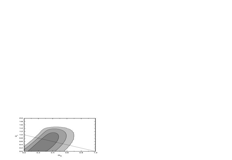
Figure 2: The top panel shows confidence interval distributions in the $\Omega_{M}-\Omega_{\Lambda}$ plane from $1\sigma$ to $3\sigma$ in an FRW cosmology. The straight line represents the flat universe. The bottom panel shows the probability versus transition redshift.

We obtain Figure 2 in a Friedmann-Robertson-Walker (FRW) cosmology with mass density $\Omega_{M}$ and vacuum energy density $\Omega_{\Lambda}$ using the GRB sample. This figure shows that $0.05<\Omega_{\rm{M}}<0.48$ at the $1\sigma$ confidence level, but $\Omega_{\Lambda}$ is poorly constrained, $\Omega_{\Lambda}<1.15$ . For a flat universe, we obtain $0.25<\Omega_{\rm{M}}<0.46$ and $0.54<\Omega_{\Lambda}<0.78$ at the $1\sigma$ confidence level. The best values of $(\Omega_{\rm{M}},\Omega_{\Lambda})$ are $(0.29,0.62)$. The transition redshift that the universe changed from the deceleration to acceleration phase is $z_{T}=0.69_{-0.12}^{+0.11}$ at the $1\sigma$ confidence level.

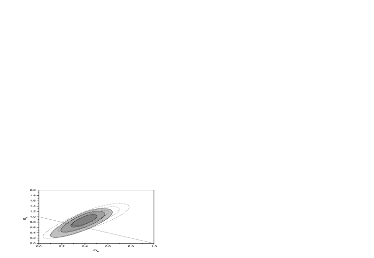
Figure 3: Constraints on $\Omega_{M}$ and $\Omega_{\Lambda}$ from $1\sigma$ to $3\sigma$ in the top panel. The dashed contours are derived from 157 SNe Ia alone and the gray ones from the GRB and SN Ia sample. The bottom panel shows the probability versus the transition redshift derived from the GRB and SN Ia sample.

We plot Figure 3 combining the GRB sample with the SN Ia sample. From this figure we find $\Omega_{M}=0.29\pm 0.03$ at the $1\sigma$ confidence level for a flat universe. The gray contours are derived from SNe Ia alone. The dashed contours are derived from the GRB and SNe Ia sample. We can see that the contours move down and become tighter as compared with the case of a combination of GRBs and SNe Ia. The result is more convincing than the one from SNe Ia alone. The transition redshift is $z_{T}=0.61_{-0.05}^{+0.06}$, which is slightly larger than the value found by considering SNe Ia alone. Figure 4 shows the confidence level derived from SN Ia sample and eight $z>1.5$ GRBs. The results are similar to those shown in Figure 3. We can conclude that an improvement of the confidence is due to the contribution of GRBs at moderate redshifts.

3.2 One-parameter dark-energy model

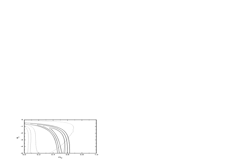
Figure 5: Constraints on $\Omega_{M}$ and $w_{0}$ from $1\sigma$ to $3\sigma$ with dark energy whose equation state is constant in the top panel. The solid contours are derived from SNe Ia alone and the long dashed contours are derived from 20 GRBs and Gold sample. The dotted contours are derived from 20 GRBs. The bottom panel shows the probability versus transition redshift derived from the GRB and SN Ia sample.

Figure 5 shows the constraints on $w_{0}$ and $\Omega_{M}$ in this dark energy model. The best values for the SN Ia and GRB sample are $\Omega_{M}=0.48_{-0.09}^{+0.07}$ and $w_{0}=-1.90^{+0.58}_{-2.85}$. The transition redshift is $z_{T}=0.50_{-0.10}^{+0.09}$. Riess et al (2004) gave $w_{0}=-1.02_{-0.19}^{+0.13}$ using SNe Ia sample with a prior of $\Omega_{M}=0.27\pm 0.04$. Firmani et al (2005) obtained $\Omega_{M}=0.44$ and $w_{0}=-1.68$ from their SNe Ia and GRB sample using the Bayesian method.

3.3 Two-parameter dark-energy model

Figure 6 exhibits the constraints on the dark energy parameters ($w_{0}$ and $w_{1}$) and transition redshift in the model of $w_{z}=w_{0}+w_{1}z$. For the SN Ia and GRB sample the best values are $w_{0}=-1.20_{-0.24}^{+0.18}$ and $w_{1}=0.85_{-0.25}^{+0.30}$ with $z_{T}=0.44_{-0.08}^{+0.09}$ at the $1\sigma$ confidence level. Firmani et al (2005) obtained $w_{0}=-1.19$ and $w_{1}=0.98$ with $z_{T}=0.55$ using their SN Ia and GRB sample. From this figure, we see that the contours plotted from the SN Ia and GRB sample move down and become tighter.

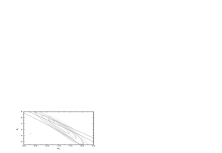
Figure 7: Constraints on $w_{0}$ and $w_{1}$ from $1\sigma$ to $3\sigma$ with dark energy whose equation state is $w_{z}=w_{0}+w_{1}z/(1+z)$ in the top panel. The long dashed contours are derived from SNe Ia alone and the dotted contours are derived from 20 GRBs and Gold sample. The diagonal lines are obtained from 20 GRBs. The bottom panel shows the probability versus transition redshift derived from the GRB and SN Ia sample.

Figure 7 presents the constraints on the dark energy parameters ($w_{0}$ and $w_{1}$) and transition redshift in the model of $w_{z}=w_{0}+w_{1}z/(1+z)$. The best values for the SN Ia and GRB sample are $w_{0}=-1.12_{-0.30}^{+0.32}$ and $w_{1}=1.90_{-1.75}^{+2.10}$ (at the $1\sigma$ confidence level)with $z_{T}=0.49_{-0.09}^{+0.07}$. From this figure we also can see that the contours plotted from the SN Ia and GRB sample move down and become tighter, being similar to Figure 4.

Figure 8 shows the constraints on the dark energy parameters ($w_{0}$ and $w_{1}$) and transition redshift in the model of $w_{z}=w_{0}+w_{1}z/(1+z)^{2}$. The best values for the SN Ia and GRB sample are $w_{0}=-1.00_{-0.25}^{+0.22}$ and $w_{1}=0.54_{-1.20}^{+0.85}$ with $z_{T}=0.37_{-0.07}^{+0.10}$ at the $1\sigma$ confidence level.

4 CONCLUSIONS and DISCUSSION

Following Liang & Zhang (2005), we have derived an empirical relation among the rest frame peak energy of the $\nu F_{\nu}$ spectrum $(E_{p}^{{}^{\prime}})$, the isotropic energy of GRB $(E_{\gamma,iso})$, and the break time of the optical afterglow light curves in the rest frame $(t_{b}^{{}^{\prime}})$ without any theoretical assumptions. The relation is $E_{\gamma,{\rm{iso}}}/10^{52}{\rm ergs}=(0.93\pm 0.25)\times(E^{{}^{\prime}}_{\rm{p}}/{\rm 100\ keV})^{1.91\pm 0.32}\times(t^{{}^{\prime}}_{\rm{b}}/1{\rm day})^{-0.93\pm 0.38}$ in a flat universe with $\Omega_{M}=0.28$ and $H_{0}=71.0$ km s^-1 Mpc^-1 for our sample with 20 GRBs. We find $0.05<\Omega_{\rm{M}}<0.48$ and $\Omega_{\Lambda}<1.15$ ($1\sigma$). For a flat universe with the cosmological constant we obtain $0.25<\Omega_{\rm{M}}<0.46$ and $0.54<\Omega_{\Lambda}<0.78$ at the $1\sigma$ confidence level. The transition redshift is $z_{T}=0.69_{-0.12}^{+0.11}$. Because of the small number of useful GRBs, we combine GRBs with SNe Ia. Using this joint sample, we find $\Omega_{M}=0.29\pm 0.03$ for a flat universe. The transition redshift is $z_{T}=0.61_{-0.05}^{+0.06}$, which is slightly larger than the value found by considering SN Ia alone. The best values for $\Omega_{M}$ and $w_{0}$ are $\Omega_{M}=0.48$ and $w_{0}=-1.90$ with the GRB and SN Ia sample in the $w_{z}=w_{0}$ model. The transition redshift is $z_{T}=0.50_{-0.10}^{+0.09}$. For the SN Ia and GRB sample the best values are $w_{0}=-1.20_{-0.24}^{+0.18}$ and $w_{1}=0.85_{-0.25}^{+0.30}$ with $z_{T}=0.44_{-0.08}^{+0.09}$ at the $1\sigma$ confidence level in the model of $w_{z}=w_{0}+w_{1}z$. The best values for the SN Ia and GRB sample are $w_{0}=-1.12_{-0.30}^{+0.32}$ and $w_{1}=1.90_{-1.75}^{+2.10}$ (at the $1\sigma$ confidence level) with $z_{T}=0.49_{-0.09}^{+0.07}$ in the model of $w_{z}=w_{0}+w_{1}z/(1+z)$. The best values for the SN Ia and GRB sample are $w_{0}=-1.00_{-0.25}^{+0.22}$ and $w_{1}=0.54_{-1.20}^{+0.85}$ with $z_{T}=0.37_{-0.07}^{+0.10}$ at the $1\sigma$ confidence level in the model of $w_{z}=w_{0}+w_{1}z/(1+z)^{2}$. The contours are tighter than those only by using the SN Ia data. From these figures a clear trend can be seen.

GRBs appear to be natural events of studying the universe at very high redshifts. They can bridge the gap between the nearby SNe Ia and the cosmic microwave background. GRBs establish a new insight on the cosmic acceleration. However the density of the circumburst medium and the efficiency of conversion of the explosion energy to gamma-rays should be assumed in the Ghirlanda relation. This is naturally overcome in the Liang & Zhang relation.

Since the empirical relation of Liang & Zhang (2005) is cosmology-dependent, we use a strategy through weighing this relation in all possible cosmological models. We find that the transition redshift varies from $0.37_{-0.07}^{+0.10}$ to $0.69_{-0.06}^{+0.05}$. Although our constraints from the GRB sample are weaker than those from SNe Ia, the constraints from the GRB and SN Ia sample are more stringent than those from the SN Ia sample. A low-$z$ GRB sample is needed to calibrate the relation in a cosmology-independent way. MIDEX-class mission, which would obtain $>$ 800 bursts in the redshift range $0.1\leq z\leq 10$ during a 2-year mission (Lamb et al. 2005), will be dedicated to using GRBs to constrain the properties of dark energy. This burst sample would enable both $\Omega_{M}$ and $w_{0}$ to be determined to $\pm 0.07$ and $\pm 0.06$ (68% C.L.), respectively, and $w_{a}$ to be significantly constrained. Probing the properties of dark energy by using GRBs is complementary (in the sense of parameter degeneracies) to other probes, such as CMB anisotropies and X-ray clusters (Lamb et al 2005). New constraints from GRBs detected in the future would improve the study of cosmology.

We thank Enwei Liang and Bing Zhang for helpful discussions, and the referee for valuable suggestions. This work was supported by the National Natural Science Foundation of China (grants 10233010 and 10221001).

Table 1: The parameters of the GRB sample used in this paper

GRB	$z$	$E_{\rm{p}}(\sigma_{E_{\rm{p}}})$	$\alpha$	$\beta$	$S_{\gamma}(\sigma_{S})$	Band	$t_{b}(\sigma_{t_{b}})$	Refs.
(1)	(2)	(3)(keV)	(4)	(5)	(6)(erg.cm-2)	(7)(keV)	(8)(days)	(9)
970828	0.9578	297.7(59.5)	-0.70	-2.07	96.0(9.6)	20-2000	2.2(0.4)	1; 5; 20; 20
980703	0.966	254(50.8)	-1.31	-2.40	22.6(2.3)	20-2000	3.4(0.5)	2; 3; 3; 3
990123	1.6	780.8(61.9)	-0.89	-2.45	300(40)	40-700	2.04(0.46)	4; 5; 5; 5
990510	1.62	161.5(16.1)	-1.23	-2.70	19(2)	40-700	1.6(0.2)	6; 5; 5; 5
990705	0.8424	188.8(15.2)	-1.05	-2.20	75.0(8.0)	40-700	1.0(0.2)	1; 19; 20; 20
990712	0.43	65(11)	-1.88	-2.48	6.5(0.3)	40-700	1.6(0.2)	6; 5; 5; 5
991216	1.02	317.3(63.4)	-1.23	-2.18	194(19)	20-2000	1.2(0.4)	7; 3; 3; 3
011211	2.14	59.2(7.6)	-0.84	-2.30	5.0(0.5)	40-700	1.56(0.02)	8; 9; 9; 8
020124	3.2	86.9(15.0)	-0.79	-2.30	8.1(0.8)	2-400	3(0.4)	10; 11; 11; 11
020405	0.69	192.5(53.8)	0.00	-1.87	74.0(0.7)	15-2000	1.67(0.52)	12; 12; 12; 12
020813	1.25	142(13)	-0.94	-1.57	97.9(10)	2-400	0.43(0.06)	13; 11; 11; 11
021004	2.332	79.8(30)	-1.01	-2.30	2.6(0.6)	2-400	4.74(0.14)	14; 11; 11; 11
021211	1.006	46.8(5.5)	-0.86	-2.18	3.5(0.1)	2-400	1.4(0.5)	15; 11; 11; 11
030226	1.986	97(20)	-0.89	-2.30	5.61(0.65)	2-400	1.04(0.12)	16; 11; 11; 11
030328	1.52	126.3(13.5)	-1.14	-2.09	37.0(1.4)	2-400	0.8(0.1)	17; 11; 11; 11
030329	0.1685	67.9(2.2)	-1.26	-2.28	163(10)	2-400	0.5(0.1)	18; 11; 11; 11
030429	2.6564	35(9)	-1.12	-2.30	0.85(0.14)	2-400	1.77(1)	19; 11; 11; 11
041006	0.716	63.4(12.7)	-1.37	-2.30	19.9(1.99)	25-100	0.16(0.04)	20; 20; 21; 21
050408	1.2357	19.93(4.0)	-1.979	-2.30	1.90(0.19)	30-400	0.28(0.17)	22; 22; 23; 23
050525a	0.606	79.0(3.5)	-0.987	-8.839	20.1(0.50)	15-350	0.28(0.12)	24; 24; 24; 24

References are in order for $z$, $E_{\rm p}^{obs}$, $[\alpha,\beta]$, $S_{\gamma}$, $t_{b}$:(1) Bloom et al. 2003; (2) Djorgovski et al. 1998; (3) Jimenez et al. 2001; (4) Kulkarni et al. 1999; (5) Amati et al. 2002; (6) Vreeswijk et al. 2001; (7)Djorgovski et al. 1999; (8) Holland et al. 2002; (9) Amati 2004; (10) Hjorth et al. 2003; (11)Sakamoto et al. 2005; (12) Price et al. 2003; (13) Barth et al. 2003; (14) Möller et al. 2002; (15) Vreeswijk et al. 2003; (16) Greiner et al. 2003; (17) Martini et al. 2003; (18)Bloom et al. 2003c; (19) Weidinger et al. 2003; (20) Butler et al. 2005. (21) Stanek et al. 2005. (22) Sakamoto et al. 2005. (23) Godet et al. 2005. (24)Blustin et al. 2005.

Figure 1: log $E\hat{}_{\gamma,iso}$ calculated by the regression method versus log $E_{\gamma,iso}$ calculated from a flat universe with $\Omega_{M}=0.28$. The line is the best regression line.

Figure 4: Constraints on $\Omega_{M}$ and $\Omega_{\Lambda}$ from $1\sigma$ to $3\sigma$ derived from 157 SNe Ia and 8 GRBs with redshifts greater than 1.5 (shown by gray contours). The dashed contours are derived from 157 SNe Ia alone.

Figure 6: Constraints on $w_{0}$ and $w_{1}$ from $1\sigma$ to $3\sigma$ with dark energy whose equation state is $w_{z}=w_{0}+w_{1}z$ in the top panel. The long dashed contours are derived from SNe Ia alone and the dotted contours are derived from 20 GRBs and Gold sample. The diagonal lines are obtained from 20 GRBs. The bottom panel shows the probability versus transition redshift derived from the GRB and SN Ia sample.

Figure 8: Constraints on $w_{0}$ and $w_{1}$ from $1\sigma$ to $3\sigma$ with dark energy whose equation state is $w_{z}=w_{0}+w_{1}z/(1+z)^{2}$ in the top panel. The long dashed contours are derived from SNe Ia alone and the dotted contours are derived from 20 GRBs and Gold sample. The diagonal lines are obtained from 20 GRBs. The bottom panel shows the probability versus transition redshift derived from the GRB and SN Ia sample.

References

- [] Allen, S. W. 2003, MNRAS. 342, 287
- [] Amati, L. 2004, Chin.J.Astron.Astrophys. 3, 455
- [] Amati, L., et al. 2002, A&A, 390, 81
- [] Barth, A. J. et al. 2003, ApJ, 584, L47
- [] Bennett, C. L. et al. 2003, ApJS, 148, 97
- [] Bloom, J. S., Morrell, N. & Mohanty, S. 2003b, GCN Report 2212
- [] Blustin, A .J. et al. 2005, astro-ph/0507515
- [] Bromm, V. & Loeb, A. 2002, ApJ, 575, 111
- [] Burrows, D. et al. 2005. GCN Reports 3222
- [] Carroll, S.M., Press, W.H. & Turner, E. L. 1992, ARA&A, 30, 499
- [] Chevallier, M. & Polarski, D. 2001, Int. J. Mod. Phys. D, 10, 213
- [] Ciardi, B. & Loeb, A. 2000, ApJ, 540, 687
- [] Dai, Z. G., Liang, E. W. & Xu, D. 2004, ApJ, 612, L101
- [] Di Girolamo, T. et al. 2005, JCAP, 4, 008
- [] Djorgovski, S. G. et al. 1998, ApJ, 508, L17
- [] Firmani, C., Ghisellini, G., Ghirlanda, G., & Avila-Reese, V. 2005, MNRAS, 360, L1
- [] Friedmann, A. S. & Bloom, J. S. 2005, ApJ, 627, 1
- [] Ghirlanda, G., Ghisellini, G., & Lazzati, D. 2004a, ApJ, 616, 331
- [] Ghirlanda, G. et al. 2004b, ApJ, 613, L13
- [] Ghirlanda, G. et al. 2005, astro-ph/0511559
- [] Godet, O. et al. 2005, GCN Reports 3222
- [] Gou, L. J., Mészáros, P., Abel, T., & Zhang, B. 2004, ApJ, 604, 508
- [] Greiner, J. et al. 2003, GCN, 2020
- [] Haislip, J. et al. 2005, Nature, submitted (astro-ph/0509660)
- [] Hjorth, J. et al. 2003, ApJ, 597, 699
- [] Holland, S. T. et al. 2002, AJ, 124, 639
- [] Jassal, H. K., Bagla, J. S. & Padmanabhan, T. 2004, MNRAS. 356, L11
- [] Jimenez, R., Band, D. L. & Piran, T. 2001, ApJ, 561, 171
- [] Kawai, N. et al. 2005, astro-ph/0512052
- [] Kulkarni, S. R. et al. 1999, Nature, 398, 389
- [] Liang, E. W. & Zhang, B. 2005, ApJ, 633, 611
- [] Liang, E. W. & Zhang, B. 2006, MNRAS, submitted (astro-ph/0512177)
- [] Lamb, D. Q. & Reichart, D. E. 2000, ApJ, 536, 1
- [] Lamb, D. Q. et al. 2005, astro-ph/0507362
- [] Linder, E, V. 2003, Phys. Rev. Lett, 90, 091301
- [] Linder, E, V. & Huterer, D. 2003, Phys.Rev.D., 67,081303
- [] Maor, I., Brustein, R. & Steinhardt P. J. 2001, Phys. Rev. Lett, 87, 049901
- [] Martini, P., Garnavich, P. & Stanek, K. Z. 2003, GCN Report 1980
- [] Mészáros, P. 2002, ARA&A, 40, 137
- [] Möller, P. et al. 2002, A&A, 396, L21
- [] Mortsell, E. & Sollerman, J. 2005, JCAP, 0506, 009
- [] Perlmutter, S. et al. 1999, ApJ, 517, 565
- [] Phillips, M. M. 1993, ApJ, 413, L105
- [] Piran, T. 1999, Phys. Rep., 314, 575
- [] Piran, T. 2004, Rev. Mod. Phys., 76, 1143
- [] Price, P. A. et al. 2003, ApJ, 589, 838
- [] Riess, A.G. et al. 1998, AJ, 116, 1009
- [] Riess, A.G. et al. 2004, ApJ, 607, 665
- [] Sakamoto, T. et al. 2005, ApJ, 629, 311
- [] Sakamoto, T., Ricker, G., Atteia, J, L. et al. 2005, GCN Reports 3189
- [] Schaefer, B. E. 2003, ApJ, 583, L67
- [] Spergel. D. N. et al. 2003, ApJS, 148, 175
- [] Stanek, K. Z. et al. 2005, ApJ, 626, L5
- [] Tegmark, M. et al. 2004, ApJ, 606, 702
- [] van Paradijs J., Kouveliotou C. Wijers, R. 2000, ARA&A, 38, 379
- [] Vreeswijk, P. M. et al. 2001, ApJ, 546, 672
- [] Vreeswijk, P., Fruchter, A., Hjorth, J. & Kouveliotou, C. 2003, GCN Report 1785
- [] Weidinger, M., Hjorth, J., Gorosabel, J., Klose, S., & Tanvir, N. 2003, GCN Report 2215
- [] Weller, J. & Albrecht, A. 2001, Phys. Rev. Lett., 86, 1939
- [] Weller, J. & Albrecht, A. 2002, Phys.Rev.D., 65, 103512
- [] Xu, D., Dai, Z. G. & Liang. E. W. 2005, ApJ, 633, 603
- [] Zhang, B. & Mészáros, P. 2004, Int. J. Mod. Phys. A, 19, 2385