Resolution requirements for simulating gravitational fragmentation using SPH

Jeans showed analytically that, in an infinite uniform-density isothermal gas, plane-wave perturbations collapse to dense sheets if their wavelength, $\lambda$, satisfies $\lambda>\lambda_{{}_{\rm JEANS}}=\left(\pi a^{2}/G\rho_{{}_{0}}\right)^{1/2}$ (where $a$ is the isothermal sound speed and $\rho_{{}_{0}}$ is the unperturbed density); in contrast, perturbations with smaller $\lambda$ oscillate about the uniform density state. Here we show that Smoothed Particle Hydrodynamics reproduces these results well, even when the diameters of the SPH particles are twice the wavelength of the perturbation. Our simulations are performed in 3-D with initially settled (i.e. non-crystalline) distributions of particles. Therefore there exists the seed noise for artificial fragmentation, but it does not occur. We conclude that, although there may be – as with any numerical scheme – ‘skeletons in the SPH cupboard’, a propensity to fragment artificially is evidently not one of them.

1 Introduction

Stars form through the collapse and fragmentation of molecular clouds. This is a highly chaotic and non-linear process; it involves many different physical effects, of which the dominant one is arguably gravitational fragmentation; and it involves a very large dynamic range of physical scales and complex geometries. Because the process is chaotic and non-linear, numerical simulations have a central role to play in understanding the interplay between the different physical effects. Because gravitational fragmentation is a critical effect, it is essential that numerical schemes are able to capture this effect properly, i.e. that true gravitational fragmentation is not suppressed by inadequate resolution, and that artificial fragmentation does not occur. Because the process involves a large dynamic range of physical scales and complex geometries, Smoothed Particle Hydrodynamics has been used extensively to simulate star formation (e.g. in 2004 alone, Bonnell, Vine & Bate, 2004; Clark & Bonnell, 2004; Delgado-Donate, Clarke & Bate, 2004a; Delgado-Donate et al., 2004b; Goodwin, Whitworth & Ward-Thompson, 2004a,b,c; Hennebelle et al., 2004; Hosking & Whitworth, 2004a,b; Jappsen & Klessen, 2004; Li, Mac Low & Klessen, 2004; Rice et al., 2004; Kurosawa et al., 2004; Price & Monaghan, 2004a,b; Schmeja & Klessen, 2004; Whitehouse & Bate, 2004).

In this paper we present a new demonstration of the ability of Smoothed Particle Hydrodynamics to simulate gravitational fragmentation properly, even at very poor resolution, using the plane-wave analysis initially performed by Jeans (1929). In Section 2, we briefly describe SPH in general, and the implementation we use in particular. In Section 3, we define – from first principles – the resolution required for simulating gravitational fragmentation, i.e. the so-called Jeans Condition. In Section 4, we describe the Jeans Test, and in Section 5, we explain how the initial conditions for the test are set up. In Section 6, we present the results of the test, emphasising how poor the resolution can be made before the results are significantly corrupted. In Section 7, we derive and demonstrate a correction term for use when the Jeans condition is not satisfied or only weakly so. In Section 8, we summarise our main conclusions.

2 Smoothed Particle Hydrodynamics

Smoothed Particle Hydrodynamics (hereafter SPH) is a Lagrangian, particle-based scheme, first formulated by Lucy (1977) and by Gingold & Monaghan (1977). The fluid is represented by an ensemble of particles having masses $m_{{}_{i}}$, positions ${\bf r}_{{}_{i}}$, velocities ${\bf v}_{{}_{i}}$, internal energies $u_{{}_{i}}$ and smoothing lengths $h_{{}_{i}}$. Apart from its gravity, the influence of particle $i$ extends only to radius $r=2h_{{}_{i}}$, and is weighted by the smoothing kernel $W(r/h_{{}_{i}})$. There need be no grids or symmetry constraints, and mass is conserved automatically, so there is no need to solve a continuity equation. Local functions of state can be evaluated at an arbitrary position ${\bf r}$ by summing contributions from all the particles $j$ whose smoothing kernel overlaps ${\bf r}$, weighted by $W(|{\bf r}-{\bf r}_{{}_{j}}|/h_{{}_{j}})$. During the evolution, ${\bf v}_{{}_{i}}$ is updated using a sum of terms representing hydrostatic, viscous, gravitational and magnetic accelerations. Similarly $u_{{}_{i}}$ can be updated using a sum of terms representing adiabatic, viscous and radiative ‘heating’. In principle, the radiative heating can be coupled to a treatment of radiation transport, but in practise this is normally very computationally expensive, and often a barotropic equation of state is used instead.

The SPH code we use here is dragon. This is an extensively tested code (Goodwin, Whitworth & Ward-Thompson, 2003a), which uses an octal spatial decomposition tree (Barnes & Hut, 1986) to speed up the calculation of gravitational accelerations and to find lists of neighbours. Gravity is kernel-softened. Particle smoothing lengths, $h_{{}_{i}}$ are adapted to give ${\cal N}_{{}_{\rm NEIB}}=50$ neighbours. A 2nd-order Runge-Kutta time-integration scheme is used, with multiple particle time-steps regulated by a Courant-like condition. The code uses time-dependent viscosity with $\alpha^{\star}_{{}_{\rm VISC}}=0.1$ (Morris & Monaghan 1997); the option exists to reduce the effective shear viscosity still further using the Balsara switch (Balsara 1995), but this option is not exercised here. Periodic boundary conditions can be imposed. If, as here, self-gravity is involved, the Ewald method is used (Hernquist et al., 1991; Klessen, 1997). Since we are imposing an isothermal equation of state (i.e. $P=a^{2}\rho$) the energy equation need not be solved.

3 Resolution requirements for gravitational fragmentation

The resolution requirements for numerical simulations of gravitational fragmentation were first addressed systematically by Truelove et al. (1997) and Bate & Burkert (1977). Truelove et al. (1997) used an Adaptive Mesh Refinement (AMR) Finite Difference (FD) code to show that grid-based codes must use cell sizes $d$ satisfying a Jeans Condition of the form $d<\lambda_{{}_{\rm JEANS}}/4$, where $\lambda_{{}_{\rm JEANS}}=(\pi a^{2}/G\rho)^{1/2}$ is the local Jeans length, $a$ is the local isothermal sound speed, and $\rho$ is the local density. If this Jeans Condition is not met in FD simulations, artificial fragmentation can occur, particularly if artificial viscosity is used.

In this context, the configuration initially explored by Boss & Bodenheimer (1979) has acquired the status of a standard test, since it is believed that the simulations of this configuration presented by Truelove et al. (1998) achieved convergence. The initial configuration involves a spherical cloud with mass $M=1{\rm M}_{{}_{\odot}}$, radius $R=5\times 10^{16}\,{\rm cm}$, uniform density $\rho=3.8\times 10^{-18}\,{\rm g}\,{\rm cm}^{-3}$, uniform temperature $T=10\,{\rm K}$ and uniform angular speed $\Omega=7.2\times 10^{-13}$ (hence ratio of thermal to gravitational energy $\alpha=0.26$ and ratio of rotational to gravitational energy $\beta=0.16$). An azimuthal $m=2$ density perturbation with fractional amplitude $A=0.1$ is then imposed and the subsequent isothermal evolution is followed. In the Truelove et al. (1998) AMR simulation of this configuration, a binary system forms, with a filament between the two components, and – as predicted by Inutsuka & Miyama (1992) – the filament does not fragment, but rather collapses to a singularity. This is in direct contrast with the earlier FD simulations of the Boss & Bodenheimer configuration reported by Burkert & Bodenheimer (1993). They used nested grids to increase the central resolution, but did not satisfy the Jeans Condition, and this resulted in fragmentation of the filament (into regularly spaced condensations with planetary masses).

The corresponding Jeans Condition for SPH has been derived by Bate & Burkert (1997), who show that SPH models gravitational fragmentation properly (i.e. artificial fragmentation is avoided and true fragmentation captured) provided (i) the gravity softening and particle smoothing have similar scales (this is achieved automatically here with kernel-softened gravity), and (ii) the local Jeans mass is resolved at all times. They suggest that the minimum mass that can be resolved by SPH is given by $M_{{}_{\rm MIN}}=2{\cal N}_{{}_{\rm NEIB}}m$, where ${\cal N}_{{}_{\rm NEIB}}\sim 50$ is the mean number of neighbours and $m$ is the mass of a single SPH particle (here assumed to be universal). In a subsequent paper (Bate, Bonnell & Bromm, 2002), this has been revised down to $M_{{}_{\rm MIN}}=1.5{\cal N}_{{}_{\rm NEIB}}m$, and therefore we have elected to put $M_{{}_{\rm MIN}}={\cal N}_{{}_{\rm NEIB}}m$ and to use the factor by which $M_{{}_{\rm JEANS}}$ exceeds $M_{{}_{\rm MIN}}$ as a measure of the accuracy of the code, Requiring

$$M_{{}_{\rm MIN}}\;=\;{\cal N}_{{}_{\rm NEIB}}\,m\;\leq\;M_{{}_{\rm JEANS}} = \frac{4\,\pi\,\left(\lambda_{{}_{\rm JEANS}}/2\right)^{3}\,\rho}{3}\;=\;\frac{\pi^{5/2}\,a^{3}}{6\,G^{3/2}\,\rho^{1/2}}$$

then reduces to

$$\rho \leq \left(\frac{\pi\,a^{2}}{G}\right)^{3}\,\left(\frac{\pi}{6\,{\cal N}_{{}_{\rm NEIB}}\,m}\right)^{2}\,,$$ (2)

or equivalently

$$\lambda_{{}_{\rm JEANS}} \geq 4\,h\,,$$ (3)

i.e. the Jeans length should exceed the diameter of an SPH particle.

Whitworth (1998) has shown analytically that with a standard smoothing kernel, and a gravitational softening length comparable to the kernel smoothing length, the only gravitational condensations which can form in SPH must (a) be genuinely gravitational unstable, and (b) be – at least approximately – resolved. Thus, failing to satisfy the Jeans Condition simply suppresses true fragmentation, rather than promoting artificial fragmentation. The present paper confirms these results.

Kitsionas & Whitworth (2002) have shown that standard SPH simulates the Boss & Bodenheimer test as well as AMR, provided sufficient particles are used to satisfy the Jeans Condition. Moreover, the number of particles can be greatly reduced (and with it the amount of memory and computation required) by implementing on-the-fly particle splitting. Despite the transient high spatial-frequency noise introduced by particle splitting, the filament between the two binary components shows no sign of fragmenting, even when the simulation is evolved to densities almost 100 times higher than Truelove et al. (1998) achieved, and the computational cost is greatly reduced. Thus, $\sim 600,000$ particles are required for standard SPH to follow this test with an isothermal equation of state to $\rho=6\times 10^{-8}\,{\rm g}\,{\rm cm}^{-3}$ (a more stringent test than attempted by Truelove et al., 1998). With particle splitting this can be achieved with $\sim 45,000$ particles initially, and fewer than $\sim 145,000$ at the end, with huge savings in the required CPU.

4 The Jeans Test

Although the Boss & Bodenheimer test is a demanding one, it does not have an analytic solution, established beyond all reasonable doubt, and therefore it is appropriate to explore a test which does have an analytic solution.

Consider a static infinite medium, with uniform density $\rho_{{}_{0}}$, and uniform and constant isothermal sound speed $a$, and assume that, even though it is self-gravitating, it is in equilibrium. This assumption is usually referred to as the ‘Jeans swindle’, since the medium cannot strictly be in self-gravitating equilibrium if the density is finite. However, in the simulations presented below the uniform density unperturbed state is effectively in equilibrium, in the sense that it can be evolved for a long time without changing.

Now suppose that the medium is perturbed so that $\rho_{{}_{0}}\rightarrow\rho_{{}_{0}}+\rho_{{}_{1}}$ and ${\bf v}_{{}_{0}}={\bf 0}\rightarrow{\bf v}_{{}_{0}}+{\bf v}_{{}_{1}}={\bf v}_{{}_{1}}$. The continuity, Euler and Poisson equations reduce to the forms

$$\frac{\partial\rho_{{}_{1}}}{\partial t} = -\,\rho_{{}_{0}}\nabla\cdot{\bf v}_{{}_{1}}$$ (4)

$$\frac{\partial{\bf v}_{{}_{1}}}{\partial t} = -\,\frac{a^{2}\,\nabla\rho_{{}_{1}}}{\rho_{{}_{0}}}\,-\,\nabla\phi_{{}_{1}}$$ (5)

$$\nabla^{2}\phi_{{}_{1}} = 4\,\pi\,G\,\rho_{{}_{1}}$$ (6)

where $\phi_{{}_{1}}$ is the gravitational potential due to the perturbed density (e.g. Binney & Tremaine, 1987). Eliminating ${\bf v}_{{}_{1}}$ and $\phi_{{}_{1}}$ from Eqns. (4) to (6) then yields

$$\frac{\partial^{2}\rho_{{}_{1}}}{\partial t^{2}}\,-\,a^{2}\,\nabla^{2}\rho_{{}_{1}}\,-\,4\,\pi\,G\,\rho_{{}_{0}}\,\rho_{{}_{1}}\;=\;0\,.$$ (7)

Substituting a plane wave of the form $\rho_{{}_{1}}({\bf r},t)=A\,\rho_{{}_{0}}\,e^{i(kx\pm\omega t)}$ in Eqn. (7) gives the dispersion relation

$$\omega_{{}_{k}}^{2}\;=\;a^{2}k^{2}\,-\,4\,\pi\,G\,\rho_{{}_{0}}\,.$$ (8)

Hence we can identify a critical Jeans wave-number,

$$k_{{}_{\rm JEANS}} = \frac{(4\pi G\rho_{{}_{0}})^{1/2}}{a}\,,$$ (9)

and correspondingly a critical Jeans wavelength,

$$\lambda_{{}_{\rm JEANS}} = \frac{2\,\pi}{k_{{}_{\rm JEANS}}}\;=\;\left(\frac{\pi\,a^{2}}{G\,\rho_{{}_{0}}}\right)^{1/2}\,,$$ (10)

separating short wavelength perturbations (which oscillate) from long wavelength perturbations (which grow).

To set up an initially stationary plane-wave perturbation, we superimpose two plane waves of equal amplitude and wavelength, travelling in opposite directions:

$$\rho_{{}_{1}}({\bf r},t) = \frac{A\,\rho_{{}_{0}}}{2}\,\left\{e^{i(kx-\omega_{{}_{k}}t)}\,+\,e^{i(kx+\omega_{{}_{k}}t)}\right\}\,,$$ (11)

$${\bf v}_{{}_{1}}({\bf r},t) = \frac{A\,\omega}{2\,k}\,\left\{e^{i(kx-\omega_{{}_{k}}t)}\,-\,e^{i(kx+\omega_{{}_{k}}t)}\right\}\,\hat{\bf e}_{{}_{x}}\,.$$ (12)

For short wavelength perturbations ($\lambda<\lambda_{{}_{\rm JEANS}}$, $k>k_{{}_{\rm JEANS}}$), the dispersion relation (Eqn. 8) indicates that $\omega^{2}$ is positive, and therefore (switching from $k$ to $\lambda$),

$$\omega_{{}_{\lambda}} = 2\,\pi\,a\,\left(\frac{1}{\lambda^{2}}\,-\,\frac{1}{\lambda_{{}_{\rm JEANS}}^{2}}\right)^{1/2}\,$$ (13)

is real and the perturbation oscillates. Taking the real parts of Eqns. (11) and (12),

$$\rho_{{}_{1}}({\bf r},t) = A\,\rho_{{}_{0}}\,\cos\left(\frac{2\,\pi\,x}{\lambda}\right)\,\cos\left(\omega_{{}_{\lambda}}t\right)\,,$$ (14)

$${\bf v}_{{}_{1}}({\bf r},t) = \frac{A\,\omega_{{}_{\lambda}}}{k}\,\sin\left(\frac{2\,\pi\,x}{\lambda}\right)\,\sin\left(\omega_{{}_{\lambda}}t\right)\,\hat{\bf e}_{{}_{x}}\,.$$ (15)

and the oscillation period is

$$T_{{}_{\lambda}} = \frac{2\,\pi}{\omega_{{}_{\lambda}}}\;=\;\left(\frac{\pi}{G\,\rho_{{}_{0}}}\right)^{1/2}\,\frac{\lambda}{(\lambda_{{}_{\rm JEANS}}^{2}-\lambda^{2})^{1/2}}\,.$$ (16)

For long wavelength perturbations ($\lambda>\lambda_{{}_{\rm JEANS}}$, $k<k_{{}_{\rm JEANS}}$), the dispersion relation (Eqn. 8) indicates that $\omega^{2}$ is negative, and therefore $\omega_{{}_{\lambda}}$ is imaginary. Defining

$$\gamma_{{}_{\lambda}} = 2\,\pi\,a\,\left(\frac{1}{\lambda_{{}_{\rm JEANS}}^{2}}\,-\,\frac{1}{\lambda^{2}}\right)^{1/2}\,,$$ (17)

we can put $\omega_{{}_{\lambda}}=i\gamma_{{}_{\lambda}}$. Then, taking the real parts of Eqns. (11) and (12), we have

$$\rho_{{}_{1}}({\bf r},t) = A\,\rho_{{}_{0}}\,\cos\left(\frac{2\,\pi\,x}{\lambda}\right)\,\cosh\left(\gamma_{{}_{\lambda}}t\right)\,,$$ (18)

$${\bf v}_{{}_{1}}({\bf r},t) = \frac{A\,\gamma_{{}_{\lambda}}}{k}\,\sin\left(\frac{2\,\pi\,x}{\lambda}\right)\,\sinh\left(\gamma_{{}_{\lambda}}t\right)\,\hat{\bf e}_{{}_{x}}\,.$$ (19)

The time for the perturbed density on the plane $x=0$ to grow from $A\rho_{{}_{0}}$ to ${\rm cosh}(1)\,A\rho_{{}_{0}}=1.54\,A\rho_{{}_{0}}$ is

$$T^{\prime}_{{}_{\lambda}} = \frac{1}{\gamma_{{}_{\lambda}}}\;=\;\left(\frac{1}{4\,\pi\,G\,\rho_{{}_{0}}}\right)^{1/2}\,\frac{\lambda}{(\lambda^{2}-\lambda_{{}_{\rm JEANS}}^{2})^{1/2}}\,.$$ (20)

Figure 1: The solid line represents one wavelength of the imposed sinusoidal plane-wave perturbation. The other lines represent the smoothing kernels used in the results displayed in Fig. 2: ${\cal R}=0.5$ (dotted line) the very well resolved case; ${\cal R}=1.0$ (dash-dot line) the marginally resolved case; and ${\cal R}=2.0$ (dashed line) the under-resolved case. The kernels are all scaled so that the integrated area under the kernel is equal to the area under the perturbation.

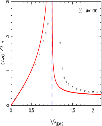
Figure 2: Characteristic timescales for the evolution of plane-wave perturbations, as a function of wavelength. The ordinate is the wavelength in units of the Jeans length, and the abscissa is the timescale in units of $(G\rho_{{}_{0}})^{-1/2}$. For perturbations which oscillate (i.e. those with $\lambda<\lambda_{{}_{\rm JEANS}}$) the oscillation period estimated from the SPH simulations is represented by an open circle. For perturbations which collapse (i.e. those with $\lambda>\lambda_{{}_{\rm JEANS}}$) the time for the peak density in the SPH simulations to increase by a factor 1.54 (see text) is represented by an open star. For reference, the analytic timescales are given by solid curves. (a) The very well resolved case, ${\cal R}=0.5$. (b) The marginally resolved case, ${\cal R}=1.0$. (c) The under-resolved case, ${\cal R}=2.0$. Note that in all cases, even the under-resolved one, wavelengths which should oscillate do oscillate (i.e. no Jeans-stable perturbations artificially collapse). In (c), the filled circles and filled stars represent simulations performed with the correction factor derived in Section 7.

5 Initial conditions

Since in both situations (low wavelength perturbations that oscillate and long wavelength perturbations that grow) the initial state is

$$\rho({\bf r},t) = \rho_{{}_{0}}\,\left\{1\,+\,A\,\cos\left(\frac{2\,\pi\,x}{\lambda}\right)\right\}\,,$$ (21)

$${\bf v}({\bf r},t) = {\bf 0}\,,$$ (22)

we set up the initial conditions as follows.

First, ${\cal N}_{{}_{\rm TOTAL}}$ particles are distributed randomly within a unit cube and settled using non–self-gravitating SPH and periodic boundary conditions. This reduces the Poissonian density fluctuations, and produces an approximately uniform, but non-crystalline, density distribution (sometimes described as glass-like). The mean smoothing length of a particle is given by

$$\bar{h} = \left(\frac{3\,{\cal N}_{{}_{\rm NEIB}}}{32\,\pi\,{\cal N}_{{}_{\rm TOTAL}}}\right)^{1/3}\;\simeq\;1.1427\,{\cal N}_{{}_{\rm TOTAL}}^{-1/3}\,,$$ (23)

where we have substituted ${\cal N}_{{}_{\rm NEIB}}=50$, and the length of the edges of the cube is equal to unity.

Second, a sinusoidal density perturbation is imposed by adjusting the unperturbed $x$-coordinate, $x_{{}_{i}}$, of each particle $i$ to a perturbed value, $x^{\prime}_{{}_{i}}$, satisfying

$$x^{\prime}_{{}_{i}}\,+\,\frac{A\,\lambda}{2\,\pi}\,\sin\left(\frac{2\,\pi\,x^{\prime}_{{}_{i}}}{\lambda}\right) = x_{{}_{i}}\,.$$ (24)

This equation must be solved numerically for $x^{\prime}_{{}_{i}}=x^{\prime}(x_{{}_{i}})$. We use a perturbation with fractional amplitude $A=0.1$.

Since periodic boundary conditions are being invoked, we can only apply perturbations which fit an integer number of wavelengths into the side of the unit cube, i.e.

$$\lambda = n_{{}_{\lambda}}^{-1}\,,$$ (25)

where $n_{{}_{\lambda}}=1,\,2,\,3,\,{\rm etc.}$.

A convenient measure of the resolution is the ratio of the mean diameter of an SPH particle, $\bar{d}=4\bar{h}$, to the wavelength of the perturbation, $\lambda=n_{{}_{\lambda}}^{-1}$, i.e.

$${\cal R}\;=\;\frac{\bar{d}}{\lambda}\;=\;n_{{}_{\lambda}}\,4\,\bar{h}\;=\;n_{{}_{\lambda}}\,\left(\frac{6\,{\cal N}_{{}_{\rm NEIB}}}{\pi\,{\cal N}_{{}_{\rm TOTAL}}}\right)\,.$$ (26)

Thus a small value of ${\cal R}$ corresponds to good resolution, and the Jeans condition (Eqn. 3) can then be rewritten in the form

$${\cal R} \leq 1\,.$$ (27)

where $\lambda=\lambda_{{}_{\rm JEANS}}$. The number of SPH particles in one Jeans mass is then

$$\frac{M_{{}_{\rm JEANS}}}{m} = \frac{{\cal N}_{{}_{\rm NEIB}}}{{\cal R}^{3}}\,.$$ (28)

The Jeans wavelength can be varied arbitrarily by changing the isothermal sound speed, $a$.

6 Test results

In Figure 1, we compare the sinusoidal perturbation with the smoothing kernel for three values of the resolution: (a) ${\cal R}=0.5$, i.e. very well resolved with $8{\cal N}_{{}_{\rm NEIB}}=400$ SPH particles in one Jeans mass; (b) ${\cal R}=1.0$, marginally resolved, with ${\cal N}_{{}_{\rm NEIB}}=50$ SPH particles in one Jeans mass; and (c) ${\cal R}=2.0$, under-resolved, with just ${\cal N}_{{}_{\rm NEIB}}/8\simeq 6$ SPH particles in one Jeans mass. We see why the resolution ${\cal R}=1.0$ is critical, in the sense that the smoothing kernel is closely matched to the perturbation (see Fig. 1), and there are just enough SPH particles to resolve a three-dimensional object.

In Figure 2 we plot the results of SPH simulations of plane-wave perturbations having different values of $\lambda/\lambda_{{}_{\rm JEANS}}$. Each panel of Fig. 2 corresponds to a different resolution, ${\cal R}$, viz. (a) ${\cal R}=0.5$, (b) ${\cal R}=1.0$, and (c) ${\cal R}=2.0$. If the perturbation oscillates, we plot with an open circle the oscillation period. If the perturbation grows, we plot as an open star the time required for the amplitude to increase by a factor ${\rm cosh}(1)=1.54$. The analytic predictions for these times (Eqns. 16 and 20) are shown as solid lines. From these plots, we can draw the following two important conclusions.

(i) There is no artificial fragmentation. Even when the resolution is poor (i.e. ${\cal R}=2.0$, Fig.2(c)), perturbations which should oscillate ($\lambda<\lambda_{{}_{\rm JEANS}}$) do oscillate, and perturbations which should grow ($\lambda>\lambda_{{}_{\rm JEANS}}$) do grow. Furthermore we should be mindful that ${\cal R}=2.0$ corresponds to a strong violation of the Jeans Condition, with only $\sim 6$ particles in a Jeans mass. It would never be tolerated in a simulation of collapse and fragmentation.

(ii) With ${\cal R}\stackrel{{\scriptstyle<}}{{\sim}}1$ (good to marginal resolution), the characteristic timescales are reproduced well, except for the cases where $\lambda\sim\lambda_{{}_{\rm JEANS}}$. Marginally Jeans stable perturbations oscillate a little too rapidly, and marginally Jeans unstable perturbations grow rather more slowly than they should.

(iii) The effect of large ${\cal R}$ (poor resolution) is to shift the asymptote separating stable wavelengths from unstable ones, from $\lambda=\lambda_{{}_{\rm JEANS}}$ to a slightly longer wavelength, i.e. to stabilise marginally Jeans unstable wavelengths, as if the temperature had been increased slightly. This is the reason for the gap on Fig. 2(c) between $\lambda/\lambda_{{}_{\rm JEANS}}=1.0$ and $\lambda/\lambda_{{}_{\rm JEANS}}=1.4$. A perturbation with (say) $\lambda=1.2\lambda_{{}_{\rm JEANS}}$ is stabilised and initially oscillates, but at the same time, because of the poor resolution, its energy is transferred to longer wavelengths modes which then become unstable with a shorter timescale than the initial perturbation, and therefore it is not possible to evaluate an oscillation period. Thus poor resolution simply suppresses the collapse of marginally unstable modes.

7 Correcting for the self-gravity of an individual SPH particle

In standard self-gravitating SPH, the mutual gravitational force between two different SPH particles is included in the equation of motion, but the self-gravity of an individual particle is not. When the Jeans mass is not well resolved, we can improve the performance of the code by correcting for the fact that part of the pressure of an SPH particle must be used to support the particle against its own self gravity , rather than pushing on other particles. To formulate this correction, consider particle $i$ in isolation. If its mass is $m_{{}_{i}}$ and its sound speed is $a_{{}_{i}}$, then

$$3\int P\,dV = 3\,m_{{}_{i}}\,a_{{}_{i}}^{2}\,,$$ (29)

where the integral is over the volume of the SPH particle. We use $a_{{}_{i}}$ because in general each SPH particle has its own sound speed which differs from that of other particles. The Virial Theorem tells us that, if the particle is to be in hydrostatic equilibrium, this integral must equal the magnitude of its self-gravitational potential energy, which is

$$|\Omega| = \frac{G\,m_{{}_{i}}^{2}\hat{W}}{h_{{}_{i}}}\,.$$ (30)

Here $h_{{}_{i}}$ is its smoothing length, and

$$\hat{W} = \int_{s=0}^{s=2}\,\cdot\,\int_{s^{\prime}=0}^{s^{\prime}=s}\,W(s^{\prime})\,4\,\pi\,s^{\prime 2}\,ds^{\prime}\,\cdot\,W(s)\,4\,\pi\,s\,ds$$ (31)

is an integral which can be worked out given the dimensionless kernel function $W(s)$. It follows that the effective sound speed squared, $a_{{}_{i,{\rm EFF}}}^{2}$, should be reduced below the true sound speed squared, $a_{{}_{i}}^{2}$, viz

$$a_{{}_{i,{\rm EFF}}}^{2}=a_{{}_{i}}^{2}-\frac{G\,m_{{}_{i}}\hat{W}}{3\,h_{{}_{i}}}\,.$$ (32)

For the standard M4 kernel which we use,

$$W(s)=\frac{1}{\pi}\left\{\;\;\begin{array}[]{ll}1-\frac{3}{2}s^{2}+\frac{3}{4}s^{3}&{\rm if}\;\;0\leq s\leq 1\,;\\ \frac{1}{4}(2-s)^{3}&{\rm if}\;\;1\leq s\leq 2\,;\\ 0&{\rm if}\;\;s>2\,.\end{array}\right.$$ (36)

(Monaghan & Lattanzio, 1985), $\hat{W}=0.505\,$.

We have repeated the simulations with ${\cal R}=2.0$, invoking this correction factor, and the results are presented as filled circles and filled stars on Fig. 2(c). As expected, the collapsing wavelengths collapse more rapidly (although still more slowly than the analytic solution).

8 Conclusions

The conclusions are very simple. SPH using the standard M4 kernel and kernel-softened gravity (i.e. the standard options) only captures fragmentation which is (a) genuine, and (b) resolved. It does not suffer from artificial fragmentation.

- (1) Balsara, D. S., 1995, JCompPhys, 121, 357
- (2) Barnes, J., Hut, P., 1986, Nature, 324, 446
- (3) Bate, M. R., Burkert, A., 1997, MNRAS, 288, 1060
- (4) Bate, M. R., Bonnell, I. A., Bromm, V., 2002, MNRAS, 332, L65
- (5) Binney, J, Tremaine, S., 1987, Galactic Dynamics (Princeton University Press; Princeton, NJ, USA)
- (6) Bonnell, I. A., Vine, S. G., Bate, M. R., 2004, MNRAS, 349, 735
- (7) Boss, A. P., Bodenheimer, P., 1979, ApJ, 234, 289
- (8) Burkert, A., Bodenheimer, P., 1993, MNRAS, 264, 798
- (9) Clark, P. C., Bonnell, I. A., 2004, MNRAS, 347, L36
- (10) Delgado-Donate, E., Clarke, C. J., Bate, M. R., 2004a, MNRAS, 347, 759
- (11) Delgado-Donate, E., Clarke, C. J., Bate, M. R., Hodgkin, S. T., 2004b, MNRAS, 351, 617
- (12) Gingold, R. A., Monaghan, J. J., 1977, MNRAS, 181, 375
- (13) Goodwin, S. P., Whitworth, A. P., Ward-Thompson, D., 2004a, A&A, 414,633
- (14) Goodwin, S. P., Whitworth, A. P., Ward-Thompson, D., 2004b, A&A, 419, 543
- (15) Goodwin, S. P., Whitworth, A. P., Ward-Thompson, D., 2004c, A&A, 423, 169
- (16) Hennebelle, P., Whitworth, A. P., Cha, S.-H., Goodwin, S. P., 2004, MNRAS, 348, 687
- (17) Hernquist, L., Bouchet, F. R, Suto, Y., 1991, ApJS, 75, 231
- (18) Hosking, J. G., Whitworth, A. P., 2004a, MNRAS, 347, 994
- (19) Hosking, J. G., Whitworth, A. P., 2004b, MNRAS, 347, 1001
- (20) Inutsuka, S., Miyama, S. M., 1992, ApJ, 388, 392
- (21) Jappsen, A.-K., Klessen, R. S., 2004, A&A, 423, 1
- (22) Jeans, J. H., 1929, Astronomy and Cosmogony (Cambridge University Press: Cambridge, UK)
- (23) Kitsionas, S., Whitworth, A. P., 2002, MNRAS, 330, 129
- (24) Klessen R., 1997, MNRAS, 292, 11
- (25) Kurosawa, R., Harries, T.J., Bate, M. R., Symington, N. H., 2004, MNRAS, 351, 1134
- (26) Li, X., Mac Low, M.-M., Klessen, R. S., 2004, ApJ, 614, L29
- (27) Lucy, L. B., 1977, AJ, 82, 1013
- (28) Monaghan, J. J., Lattanzio, J. C., 1985, A&A, 149, 135
- (29) Morris, J. P., Monaghan, J. J., 1997, JCompPhys, 136, 41
- (30) Price, D. J., Monaghan, J. J., 2004a, MNRAS, 348, 123
- (31) Price, D. J., Monaghan, J. J., 2004b, MNRAS, 348, 139
- (32) Rice, W. K. M., Lodato, G., Pringle, J. E., Armitage, P. J., Bonnell, I. A., 2004, MNRAS, 355, 543
- (33) Schmeja, S., Klessen, R. S., 2004, A&A, 419, 405
- (34) Truelove, J. K., Klein, R. I., McKee, C. F., Holliman, J. H., II, Howell, L. K., Greenough, J. A., 1997, 489, L179
- (35) Truelove, J. K., Klein, R. I., McKee, C. F., Holliman, J. H., II, Howell, L. K., Greenough, J. A., Woods, D. T., 1998, ApJ 495, 821
- (36) Whitehouse, S. C., Bate, M. R., 2004, MNRAS, 353, 1078
- (37) Whitworth, A. P. 1998, MNRAS, 296, 442