Very Efficient Methods for
Multilevel Radiative Transfer
in Atomic and Molecular Lines

Abstract

The development of fast numerical methods for multilevel radiative transfer (RT) applications often leads to important breakthroughs in astrophysics, because they allow the investigation of problems that could not be properly tackled using the methods previously available. Probably, the most familiar example is the so-called Multilevel Accelerated $\Lambda$-Iteration (MALI) technique of Rybicki & Hummer for the case of a local approximate operator, which is based on Jacobi iteration. However, there are superior operator-splitting methods, based on Gauss-Seidel (GS) and Successive Overrelaxation (SOR) iteration, which provide a dramatic increase in the speed with which non-LTE multilevel transfer problems can be solved in one, two and three-dimensional geometries. Such RT methods, which were introduced by Trujillo Bueno & Fabiani Bendicho ten years ago, are the main subject of the first part of this paper. We show in some detail how they can be applied for solving multilevel RT problems in spherical geometry, for both atomic and molecular line transitions. The second part of the article addresses the issue of the calculation of the molecular number densities when the approximation of instantaneous chemical equilibrium turns out to be inadequate, which happens to be the case whenever the dynamical time scales of the astrophysical plasma under consideration are much shorter than the time needed by the molecules to form.

1 Introduction

Astrophysical plasma spectroscopy is a fascinating but very complex research field because non-equilibrium physics is required. First, for given atomic or molecular number densities at each point within the astrophysical plasma under consideration, we have the problem of how to calculate the population numbers of the levels included in the atomic or molecular model. Second, it is also important to remember that the atomic and/or molecular number densities themselves are not always given by the instantaneous values of the physical conditions of the plasma (e.g., kinetic temperature, density), simply because such conditions may be changing rapidly with time as as result of magneto-hydrodynamical processes. Therefore, for instance, it may be “dangerous” to infer chemical abundances in stellar atmospheres by computing the molecular number densities via the approximation of instantaneous chemical equilibrium.

The present keynote article addresses these two aspects of astrophysical plasma spectroscopy, with emphasis on the increasingly attractive topic of non-LTE radiative transfer in molecular lines (e.g., note that in the very near future the Herschell Space Observatory of ESA is expected to be fully operative).

2 The Non-LTE Multilevel Radiative Transfer Problem

2.1 Basic equations

The standard multilevel radiative transfer problem requires the joint solution of the radiative transfer (RT) equation (which describes the radiation field) and the kinetic equations (KE) for the atomic or molecular level populations (which describe the excitation state). The numerical solution of this non-local and non-linear problem requires to discretize the model atmosphere in NP points, where the physical properties are assumed to be known. The standard multilevel RT problem consists in obtaining the population $n_{j}$ of each of the $j=1,2,\ldots,\mathrm{NL}$ levels included in the atomic/molecular model that are consistent with the radiation field within the stellar atmosphere. This radiation field has contributions from possible background sources and from the radiative transitions in the given atomic/molecular model.

Making the usual assumption of statistical equilibrium, the rate equation for each level $i$ at each spatial point reduces to (Socas-Navarro & Trujillo Bueno 1997):

$$\sum_{j<i}{\Gamma}_{ji}\,-\,\sum_{j>i}{\Gamma}_{ij}\,+\,\sum_{j\neq i}{n_{j}C_{ji}}-n_{i}\sum_{j\neq i}{C_{ij}}=0,$$ (1)

where $C_{ij}$ is the collisional rate between levels $i$ and $j$ and $\Gamma_{lu}$ is the net radiative rate in the transition from a bound lower level $l$ to an upper level $u$:

$$\Gamma_{lu}\,=\,n_{l}R_{lu}\,-\,n_{u}\,R_{ul}\,,$$ (2)

with $R_{ij}$ the radiative rates. Given that Eqs. (1) are not linearly independent, we replace one of them by the particle conservation law:

$$\sum_{i}n_{i}=n_{\mathrm{total}},$$ (3)

where $n_{\mathrm{total}}$ is the total number density of the species under consideration. The resulting system can be formally written as:

$$\bf A\cdot n=f,$$ (4)

where $\bf A$ is a matrix of size NL$\times$NL whose elements contain the collisional and radiative rates (except for one of the rows that contains 1 due to the conservation law), $\bf f$ is a vector of length NL with zeros except for the $n_{\mathrm{total}}$ value of the conservation law, and $\bf n$ is a vector containing the population of each level. The result of grouping together the sets of Eqs. (4) for all the NP grid points of the atmosphere can be symbolically represented as

$$\bf L\cdot n=f,$$ (5)

where $\mathbf{f}$ is a known vector of size NP$\times$NL, $\mathbf{n}$ is a vector of the same length with the populations of the NL levels for each of the NP points and $\mathbf{L}$ is a block-diagonal matrix such that each of its NP blocks of size NL$\times$NL is given by the matrix $\mathbf{A}$ of Eq. (4).

The collisional rates are assumed to be known and given by the local physical conditions of the atmosphere. On the other hand, the net radiative rates $\Gamma_{lu}$ depend on the radiation field within the stellar atmosphere. For bound-bound transitions

$$\Gamma_{lu}\,=(n_{l}B_{lu}-n_{u}B_{ul}){\bar{J}}_{lu}\,-\,n_{u}A_{ul},$$ (6)

where $A_{ul}$, $B_{ul}$ and $B_{lu}$ are the Einstein coefficients. A key quantity is $\bar{J}_{lu}$, which is the frequency averaged mean intensity weighted by the line absorption profile:

$$\bar{J}_{lu}=\frac{1}{4\pi}\int d\mathbf{\Omega}\int d\nu\phi_{lu}(\nu,\mathbf{\Omega})I_{\nu\mathbf{\Omega}},$$ (7)

where $\phi_{lu}$ and $I_{\nu\bf\Omega}$ are, respectively, the normalized line profile and the specific intensity at frequency $\nu$ and direction $\bf\Omega\rm$. The specific intensity is governed by the radiative transfer equation, which can be formally solved if we know the variation of the opacity ($\chi_{\nu}$) and of the source function ($\epsilon_{\nu}/\chi_{\nu}$, being $\epsilon_{\nu}$ the emission coefficient) in the medium. Once the stellar atmosphere is discretized, the specific intensity can be written formally as

$$\bf I_{\nu\mathbf{\Omega}}=\bf\Lambda_{\nu\mathbf{\Omega}}\left[\bf S_{\nu}\right]+\mathcal{\bf T}_{\nu\mathbf{\Omega}},$$

where $\mathcal{\bf T}_{\nu\mathbf{\Omega}}$ is a vector that accounts for the contribution of the boundary conditions to the intensity at each spatial point of the discretized medium, $\bf S_{\nu}$ is the source function vector and $\bf\Lambda_{\nu\mathbf{\Omega}}$ is an operator whose element $\Lambda_{\nu\mathbf{\Omega}}(i,j)$ gives the response of the radiation field at point “$i$” due to a unit-pulse perturbation in the source function at point “$j$”.

Since the radiative transfer equation couples different parts of the atmosphere and the absorption and emission properties at all the spatial points depend on the level populations, the RT problem is both non-local and non-linear. Therefore, the system of Eqs. (4) represents a highly non-linear problem (i.e., the operator $\mathbf{A}$ depends implicitly on $\mathbf{n}$). This non-linearity makes it necessary to apply suitable iterative methods.

2.2 Formal solution in spherical geometry

The equation that describes the radiative transfer in a spherically symmetric atmosphere where the physical conditions vary only along the radial direction is (e.g., Mihalas 1978):

$$\mu\frac{\partial I_{\nu}(r,\mu)}{\partial r}+\frac{\left(1-\mu^{2}\right)}{r}\frac{\partial I_{\nu}(r,\mu)}{\partial\mu}=\epsilon_{\nu}(r,\mu)-\chi_{\nu}(r,\mu)I_{\nu}(r,\mu),$$ (8)

where $r$ is the radial coordinate and $\mu$ the cosine of the angle between the radial direction and the ray. This partial differential equation (PDE) can be reduced to a set of ordinary differential equations (ODE) if solved along the characteristics of the PDE. In this case, the characteristic curves (parameterized by $t$) are straight lines with constant impact parameter $p$:

$$\frac{\partial r}{\partial t} = \mu$$

$$\frac{\partial\mu}{\partial t} = \frac{1-\mu^{2}}{r}.$$ (9)

In order to solve the RT equation in spherical geometry, we apply the parabolic short-characteristics (SC) method (Kunasz & Auer 1988; Auer & Paletou 1994; Auer, Fabiani Bendicho & Trujillo Bueno 1994) along each ray of constant impact parameter. As shown by Trujillo Bueno & Fabiani Bendicho (1995), the SC method allows an efficient implementation of the fast iterative methods based on the Gauss–Seidel iterative scheme. The parabolic SC method assumes that the variation of the source function with the optical depth along the ray under consideration has a parabolic behavior between each three consecutive points. Consider the upwind point M, the point O where the intensity is being calculated and the downwind point P. The source function at each of such consecutive points can be easily calculated from the current values of the level populations. The intensity $I_{\mathrm{M}}$ at the upwind point M is also known from previous steps. Taking into account that the formal solution of the radiative transfer equation is given by

$$I_{\mathrm{O}}=I_{\mathrm{M}}e^{-\Delta\tau_{\mathrm{MO}}}+\int_{0}^{\Delta\tau_{\mathrm{MO}}}S(t)e^{-(\Delta\tau_{\mathrm{MO}}-t)}dt,$$ (10)

it is easy to obtain the following formula (Kunasz & Auer 1988):

$$I_{\mathrm{O}}=I_{\mathrm{M}}e^{-\Delta\tau_{\mathrm{MO}}}+\Psi_{\mathrm{M}}S_{\mathrm{M}}+\Psi_{\mathrm{O}}S_{\mathrm{O}}+\Psi_{\mathrm{P}}S_{\mathrm{P}}.$$ (11)

The quantities $\Psi_{\mathrm{M,O,P}}$ are functions of the optical distances $\Delta\tau_{\mathrm{MO}}$ between the upwind point M and the point O and of the optical distance $\Delta\tau_{\mathrm{OP}}$ between the point O and the downwind point P, while $S_{\mathrm{M,O,P}}$ are the values of the source function at points M, O and P, respectively. We can build a similar formula assuming that the source function varies linearly between points M and O, which is used only at the boundary grid points for rays going out of the boundaries. In this case, the last term of Eq. (11) disappears and $\Psi_{\mathrm{M}}$ and $\Psi_{\mathrm{O}}$ only depend on $\Delta\tau_{\mathrm{MO}}$. Note that $\Delta\tau_{\mathrm{MO}}{\approx}(\chi_{\mathrm{M}}+\chi_{\mathrm{O}})/2$ and $\Delta\tau_{\mathrm{OP}}{\approx}(\chi_{\mathrm{O}}+\chi_{\mathrm{P}})/2$, with $\chi_{i}$ the opacity at point $i$ (which depends on the lower-level population at point $i$).

2.3 Iterative methods for radiative transfer applications

The basic idea behind an iterative method for the solution of a nonlinear problem is to start from an estimation of the solution (ideally as close to the final solution as possible) and then to perform successive corrections to the current estimation until the final solution is found. Iterative methods for multilevel transfer problems obey the same structure. Consider the solution of Eqs. (4) at each of the NP spatial points. We start from an estimate, $\bf n^{\rm old}$, of the atomic or molecular level populations at each point. If this estimate is not the exact solution of the problem, we have a nonzero residual

$$\bf r=f-A^{\rm old}\cdot n^{\rm old}\neq 0,$$ (12)

where the superscript “old” indicates that the radiative rates of the operator $\bf A^{\rm old}$ have to be calculated by solving the RT equation using the previous estimation of the populations (i.e., using $\bf n^{\rm old}$). This matrix is built, for every point in the atmosphere, by using also the appropriate collisional rates of the chosen atomic/molecular model. The aim is to find the correction, $\mathbf{\delta n}$, such that the estimation:

$$\bf n^{\rm new}=n^{\rm old}+\delta n$$ (13)

gives a zero residual and, therefore,

$$\bf A^{\rm new}\cdot\delta n=f-A^{\rm new}\cdot n^{\rm old}.$$ (14)

Note that this equation cannot be directly solved because it is still nonlinear and similar to the original Eq. (4); hence it is not possible to solve the problem in one single step. Therefore, we have to obtain approximate corrections in order to arrive to the self-consistent solution iteratively. The different iterative methods applied to the solution of multilevel radiative transfer problems differ in the way one manages to build, at each iterative step, a linear system of equations whose solution gives approximate corrections to the level populations. An efficient iterative method should account for the non-locality and the radiative couplings of the problem (see Socas-Navarro & Trujillo Bueno 1997).

2.3.1 The $\Lambda$-iteration method

This method is the most direct and simple one. It consists in solving Eq. (14) by calculating the radiative rates at each point in the atmosphere using the populations from the previous iterative step (i.e., $\bf n^{\rm old}$). Therefore, the corrections to the estimation of the populations can be obtained from:

$$\bf A^{\rm old}\cdot\delta n=r.$$ (15)

Note that the mean intensity $\bar{J}_{lu}$ at each spatial point is obtained by solving the RT equation using the $\mathbf{n}^{\mathrm{old}}$ values of the populations at all the points of the computational grid. In this way, at each iterative step the nonlinear system is transformed into a linear one, which can be solved easily to obtain the approximate corrections to the populations. This procedure is iterated until convergence. Although very simple and easy to code, the $\Lambda$-iteration method has a serious drawback, which is its very poor convergence rate in optically thick media. This is due to the fact that this method is equivalent to assuming that the radiation field does not react to the perturbations in the populations (see Socas-Navarro & Trujillo Bueno 1997). For example, for the case of bound-bound transitions such an unrealistic assumption implies that the expression of Eq. (6) is taken equal to

$$\Gamma_{lu}\,=(n_{l}^{\rm new}B_{lu}-n_{u}^{\rm new}B_{ul}){\bar{J}}_{lu}^{\rm old}\,-\,n_{u}^{\rm new}A_{ul}.$$ (16)

In fact, when this approximate expression for the net radiative rate is introduced in Eq. (1) we obtain Eq. (15). In any case, we point out that the $\Lambda$-iteration method is useful for optically thin problems (e.g., Bernes 1979, Uitenbroek 2000).

2.3.2 The Multilevel Accelerated $\Lambda$-iteration Method (MALI)

MALI is a clever modification of the $\Lambda$-iteration method, which implies a much higher convergence rate (Cannon 1973; Olson, Auer & Buchler 1986; Rybicki & Hummer 1991, 1992; Auer, Fabiani Bendicho & Trujillo Bueno 1994). There are several methods to achieve the required linearity in the system of Eqs. (14) at each iterative step. The most powerful ones are linearization (Auer & Mihalas 1969; Scharmer & Carlsson 1985) and preconditioning (Rybicki & Hummer 1991, 1992). Socas-Navarro & Trujillo Bueno (1997) showed that both schemes are equivalent, but that the preconditioning strategy with a local approximate operator guarantees positive populations. The preconditioning approach with a local approximate operator is nowadays the most used due to its simplicity and good performance. It is usually referred to as Multilevel-ALI (MALI).

As pointed out by Socas-Navarro & Trujillo Bueno (1997) this method takes into account the local response of the radiation field to the source function perturbations. For example, for the case of bound-bound transitions the expression of Eq. (6) takes the form

$$\Gamma_{lu}\,=(n_{l}^{\rm new}B_{lu}-n_{u}^{\rm new}B_{ul})({\bar{J}}_{lu}^{\rm old}-{\bar{\Lambda}}_{lu}^{*}S_{lu}^{\rm old})\,-\,n_{u}^{\rm new}A_{ul}(1-{\bar{\Lambda}}_{lu}^{*}),$$ (17)

where $S_{lu}^{\mathrm{old}}$ is the line source function computed using $\mathbf{n}^{\mathrm{old}}$. When this new approximate expression for the net radiative rate is introduced in Eq. (1) the resulting linearized system of equations is

$$\bf A_{\rm MALI}^{\rm old}\cdot\delta n=r,$$ (18)

which is similar to Eq. (15), but with the crucial difference that the elements of $\bf A_{\rm MALI}^{\rm old}$ now account for the information provided by the approximate $\Lambda$-operator through the quantity

$$\bar{\mathbf{\Lambda}}_{lu}^{*}=\frac{1}{4\pi}\int d\mathbf{\Omega}\int d\nu\phi_{lu}(\nu)\mathbf{\Lambda}_{\nu\mathbf{\Omega}}^{*}r_{lu}^{\mathrm{old}},$$ (19)

where $r_{lu}^{\mathrm{old}}$ is the frequency-dependent line strength given by

$$r_{lu}^{\mathrm{old}}=\frac{\chi_{lu}^{\mathrm{old}}\phi_{lu}(\nu)}{\chi_{lu}^{\mathrm{old}}\phi_{lu}(\nu)+\chi_{c}},$$ (20)

with $\chi_{lu}^{\mathrm{old}}$ the line opacity computed with $\mathbf{n}^{\mathrm{old}}$ and $\chi_{c}$ the background opacity. When the approximate operator is chosen equal to the diagonal of the full operator $\bf\Lambda_{\nu\mathbf{\Omega}}$, the computational time per iteration is similar to that of the $\Lambda$-iteration scheme.

The implementation of the MALI method for the solution of RT problems in spherical geometry can be easily carried out with the aid of the short-characteristics formal solver. We need to evaluate the mean intensity, $\bar{J}_{lu}$, and the approximate operator, $\bar{\mathbf{\Lambda}}_{lu}^{*}$, for each transition. The following steps describe the implementation details:

1. Incoming part. We start the integration of the RT equation from the outer boundary surface along rays with constant impact parameter $p$ using the appropriate boundary condition. If the outer boundary condition has a dependence on the angle $\mu$, then each characteristics will have a different boundary condition $I(R,\mu)$. The intensity is then propagated inwards along each ray applying the formal solution as established by the parabolic short-characteristics method. This process is carried out for each ray until the inner boundary surface is reached (for the rays that intersect the core) or until tangentially reaching the shell with $r=p$ (for the rays that do not intersect the core). Such calculations give us the information required to obtain the angular dependence of the incoming radiation field and its contribution to the mean intensity:

   $$\bar{J}_{lu}(\mathrm{in},r_{i})=\frac{1}{2}\int_{-1}^{0}d\mu\int d\nu\phi_{lu}(\nu)I(r_{i},\mu),$$ (21)

   where we have explicitly indicated that it is the contribution of the incoming radiation. The contribution of the incoming radiation to the approximate $\mathbf{\Lambda}_{\nu\mathbf{\Omega}}^{*}$ operator is also calculated. Since for this operator we have chosen the diagonal of the full operator, it represents the response of the mean intensity to a unit pulse perturbation in the source function at the point O under consideration. For the case of a bound-bound transition with a fixed background continuum, it can be calculated as:

   $$\bar{\Lambda}^{*}_{ii}(\mathrm{in},r_{i})=\frac{1}{2}\int_{-1}^{0}d\mu\int d\nu\phi_{lu}(\nu)\left[I_{\mathrm{M}}e^{-\Delta\tau_{\mathrm{MO}}^{\mathrm{old}}}+\Psi_{\mathrm{O}}^{\mathrm{old}}(\mathrm{in})\right]r_{lu}^{\mathrm{old}},$$ (22)

   where $\Psi_{\mathrm{O}}$ is one of the coefficients of the short-characteristics formula (11). Although $I_{\mathrm{M}}$ is usually taken equal to zero, in reality it is a small negative contribution which can be easily calculated (see the shaded area of Fig. 1). The reason is that the unit pulse perturbation at point O produces a residual intensity at point M coming from the application of the parabolic SC formula to the points L, M and O, as indicated in Fig. 1.

   

   Figure 1: The unit pulse perturbation in the source function at point O necessary for the calculation of the $\mathbf{\Lambda}_{\nu\mathbf{\Omega}}^{*}$ operator produces a residual intensity at point M. This contribution comes from the application of the parabolic SC formula at points L, M and O, where point L precedes point M along the ray.

2. Outgoing part. We apply the inner boundary condition for the rays that intersect the core and continue integrating the RT equation along the outgoing rays until reaching the external boundary surface. The contribution of the outgoing radiation field to the mean intensity can be obtained as:

   $$\bar{J}_{lu}(\mathrm{out},r_{i})=\frac{1}{2}\int_{0}^{1}d\mu\int d\nu\phi_{lu}(\nu)I(r_{i},\mu),$$ (23)

   and similarly for the approximate operator.

When this process is carried out for all the spectral lines of the atomic/molecular model, the mean intensity $\bar{J}_{lu}$ and the $\bar{\mathbf{\Lambda}}_{lu}^{*}$ operator are available at each spatial point. We can then build the system matrix $\bf A_{\rm MALI}^{\rm old}$ for each point and obtain the approximate corrections to the populations.

2.3.3 The Multilevel Gauss–Seidel Method (MUGA)

This method was developed by Trujillo Bueno & Fabiani Bendicho (1995). The paper by Fabiani Bendicho, Trujillo Bueno & Auer (1997) gives a suitable summary of its application to the multilevel problem in cartesian coordinates, including a detailed analysis of its convergence rate and performance. Although the computational time per iteration is similar to that of MALI, MUGA has a much better convergence behavior. The key point of the Gauss–Seidel method for RT applications is that one obtains the convergence rate of an upper or lower triangular approximate $\Lambda$-operator without having to build and/or invert this triangular operator. To this end, once the radiation field is known at the atmospheric point being considered, the population correction can be made directly using Eqs. (18). Then, if these new populations are taken into account when calculating the radiation field at the next spatial grid point, the resulting scheme turns out to be equivalent to that of the Gauss-Seidel method, which has a higher convergence rate than Jacobi’s method (Trujillo Bueno & Fabiani Bendicho 1995; Trujillo Bueno 2003). It is important to clarify that MUGA, contrary to what happens with MALI, requires an specific order of the loops over transitions, angles (equivalently, rays with constant impact parameter in the spherically symmetric case) and spatial points when propagating the radiation. The most external loop is the one over directions, first going inwards and then ouwards. The next one is the loop over spatial points, followed by the loop over transitions. The most internal ones are the loops over angles and frequencies. The reason is that we need to evaluate the mean intensity for all the radiative transitions in order to be able to perform the population correction before advancing to the following point of the spatial grid. This ordering is shown in a pseudo-code manner in the following algorithm:

Algorithm 1 The MUGA scheme

  for directions do {directions are incoming and outgoing}

     for spatial points do

        for transitions do

           for angles do

              for frequencies do

                 Propagate radiation using parabolic SC

              end for

           end for

           Calculate mean intensity of the given transition

        end for

        Carry out population correction

     end for

  end for

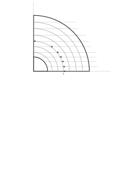
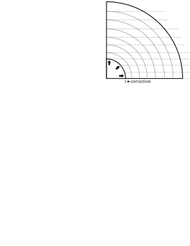
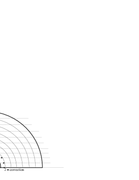
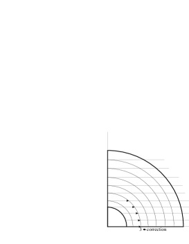
Figure 2: Schematic representation of the Gauss-Seidel iterative scheme in its incoming and outgoing phases. Note that the inner boundary is the shell $i=1$, while the external boundary is the shell $i=\mathrm{NP}$.

MUGA can be extended to spherical geometry as follows:

1. Incoming part. The formal integration of the RT equation along each ray of constant impact parameter $p$ is started at the outer boundary. This process is schematized in the upper left panel of Fig. 2. Note that the intensity can be propagated simultaneously along all the rays. The integration along each ray is done using short-characteristics, calculating the intensity at each shell until the ray intersects the central core or arrives tangent to the shell $r=p$. Once the incoming intensity at every intersection point between the shells and the whole set of rays is known, the contribution to the mean intensity of the incoming rays ($\mu<0$) can be calculated.

2. Outgoing part. When the contribution to the mean intensity from the incoming radiation is known, the boundary condition at the inner core can be applied to get the contribution of the outgoing radiation to the mean intensity in all the radiative transitions, thus allowing us to solve the linear system of Eqs. (18) to get the population correction at the inner core. The schematic representation of this step is shown in the upper right panel of Fig. 2. With these improved level populations, one can propagate the intensity outwards until the next shell and get the mean intensity there for each of the transitions [what Trujillo Bueno & Fabiani Bendicho (1995) call $\bar{J}_{lu}^{\mathrm{old\&new}}$], which then allows us to solve the linear system of Eqs. (18) to obtain the new populations corresponding to this shell. The procedure is repeated until arriving to the outer boundary. This process is schematized in the lower left and right panels of Fig. 2. The “old&new” label of the mean intensity is used to indicate clearly that the value of the mean intensity $\bar{J}_{lu}$ at shell $n$ is obtained by using the new population at the shells with $r<r_{n}$, contrarily to what happens with the MALI method, where the mean intensity is calculated always by using the “old” population estimation. Consequently, the final system to be solved at each shell is:

   $$\bf A_{\rm GS}^{\rm old\&new}\delta n=r,$$ (24)

   where the coefficients of $\bf A_{\rm GS}^{\rm old\&new}$ are similar to those of $\bf A_{\rm MALI}$ but calculated one spatial point after the other as summarized above.

As explained in detail by Trujillo Bueno & Fabiani Bendicho (1995) for the plane–parallel case, two corrections have to be performed in order to obtain a true GS iteration. Let us assume that we have already obtained the new populations at point $i$ and that we want to calculate the new populations at point $i+1$. The corrections, graphically schematized in Figure 3, are the following:

1. The first one, represented in the left panel of Fig. 3, affects the incoming radiation field at point $i+1$ after the population correction is performed at point $i$ during the outgoing pass. Since the parabolic SC formal solver is being used, the radiation field at point $i+1$ depends on the absorption and emission properties at points $i$, $i+1$ and $i+2$. The incoming radiation field at $i+1$ had been calculated using the “old” populations at point $i$. Since we have already a new estimation of the populations at point $i$, we have to correct the incoming radiation field as illustrated in Fig 3. We indicate in grey those points for which we have a “new” estimation of the populations, while those points with the “old” populations are marked in black. The intensity at point $i+1$ for the incoming ray with impact parameter $p$ was calculated according to the formula:

   $$\begin{split}I_{i+1}^{\mathrm{old}}(\mathrm{in},p)&=I_{i+2}^{\mathrm{old}}(\mathrm{in},p)e^{-\Delta\tau_{i+2,i+1}^{\mathrm{old}}}\\ &+\Psi_{i+2}^{\mathrm{old}}(\mathrm{in})S_{i+2}^{\mathrm{old}}(p)+\Psi_{i+1}^{\mathrm{old}}(\mathrm{in})S_{i+1}^{\mathrm{old}}(p)+\Psi_{i}^{\mathrm{old}}(\mathrm{in})S_{i}^{\mathrm{old}}(p),\end{split}$$ (25)

   which has to be replaced with:

   $$\begin{split}I_{i+1}^{\mathrm{new}}(\mathrm{in},p)&=I_{i+2}^{\mathrm{old}}(\mathrm{in},p)e^{-\Delta\tau_{i+2,i+1}^{\mathrm{old}}}\\ &+\Psi_{i+2}^{\mathrm{new}}(\mathrm{in})S_{i+2}^{\mathrm{old}}(p)+\Psi_{i+1}^{\mathrm{new}}(\mathrm{in})S_{i+1}^{\mathrm{old}}(p)+\Psi_{i}^{\mathrm{new}}(\mathrm{in})S_{i}^{\mathrm{new}}(p),\end{split}$$ (26)

   since the populations at point $i$ have just been corrected. This correction in the specific intensity is performed for each ray and is then taken into account when calculating the mean intensity at point i+1.

   

   

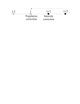
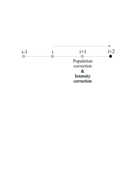
   Figure 3: Corrections needed for obtaining a true Gauss-Seidel iteration when using the parabolic SC method. The left panel shows the corrections to the incoming radiation field at point $i+1$ due to the population correction obtained previously at point $i$. The right panel shows the corrections to the outgoing radiation field at point $i+1$ after performing the population correction at this point $i+1$. Note that the inner boundary is at point $i=1$ and the outer boundary is at point $i=\mathrm{NP}$.

2. The second correction, represented in the right panel of Fig. 3, is necessary once a new estimation of the populations is available for point $i+1$. Since the outgoing radiation field at point $i+1$ has been obtained with the “old” populations at this point, it has to be corrected in order to obtain the true value of the outgoing radiation field at point $i+1$ before moving to the next point $i+2$. Therefore, the outgoing intensity at point $i+1$, which had been obtained using:

   $$\begin{split}I_{i+1}^{\mathrm{old}}(\mathrm{out},p)&=I_{i}^{\mathrm{new}}(\mathrm{out},p)e^{-\Delta\tau_{i,i+1}^{\mathrm{new}}}\\ &+\Psi_{i}^{\mathrm{new}}(\mathrm{out})S_{i}^{\mathrm{new}}(p)+\Psi_{i+1}^{\mathrm{new}}(\mathrm{out})S_{i+1}^{\mathrm{old}}(p)+\Psi_{i+2}^{\mathrm{new}}(\mathrm{out})S_{i+2}^{\mathrm{old}}(p),\end{split}$$ (27)

   has to be replaced by:

   $$\begin{split}I_{i+1}^{\mathrm{new}}(\mathrm{out},p)&=I_{i}^{\mathrm{new}}(\mathrm{out},p)e^{-\Delta\tau_{i,i+1}^{\mathrm{new}}}\\ &+\Psi_{i}^{\mathrm{new}}(\mathrm{out})S_{i}^{\mathrm{new}}(p)+\Psi_{i+1}^{\mathrm{new}}(\mathrm{out})S_{i+1}^{\mathrm{new}}(p)+\Psi_{i+2}^{\mathrm{new}}(\mathrm{out})S_{i+2}^{\mathrm{old}}(p),\end{split}$$ (28)

   since now the populations at point $i+1$ have just been corrected.

These corrections are applied consecutively while computing the outgoing radiation field until reaching the outer boundary surface.

Summarizing, when such two corrections are applied to the iterative scheme, a true Gauss-Seidel iteration is obtained once the specific intensity of the radiation field is propagated from the outer to the inner boundary, and again to the outer one. This MUGA scheme leads to a convergence rate a factor 2 higher than that corresponding to the MALI method. The main advantage of this GS-based iterative scheme is that it has the convergence properties of a triangular $\mathbf{\Lambda}_{\nu\mathbf{\Omega}}^{*}$-operator, but neither the construction nor the inversion of this approximate operator has to be performed. Therefore, it is also suitable for 2D and 3D multilevel radiative transfer (see Fabiani Bendicho & Trujillo Bueno 1999).

As pointed out by Trujillo Bueno & Fabiani Bendicho (1995) and by Trujillo Bueno (2003), the increase in the convergence rate can be enhanced to a factor of 4 if the previous corrections are applied, not only when the radiation field is being propagated outwards, but also when it is being propagated inwards. In this way, each incoming+outgoing pass produces two GS iterations. Some examples of the application of this “up+down” strategy to polarized radiative transfer can be found in Trujillo Bueno & Manso Sainz (1999).

2.3.4 The Multilevel Successive Overrelaxation Method (MUSOR)

The Successive Overrelaxation method (SOR) has been also proposed by Trujillo Bueno & Fabiani Bendicho (1995) for the solution of non-LTE RT problems. The solution process is exactly the same as in MUGA, since the only difference lies on the level population correction. In the SOR method, a parameter $\omega$ is introduced to overcorrect the population, thus allowing for some kind of anticipation of the future corrections. This scheme can be written as

$$\bf A_{\rm GS}^{\rm old\&new}\cdot\delta n = \bf r$$

$$\bf n^{\rm new} = \bf n^{\rm old}+\omega\delta n,$$ (29)

where the $\omega$ parameter has a value between 1 and 2 in order to produce the overcorrection. The MUGA method is therefore a particular case of the MUSOR scheme (see Trujillo Bueno & Fabiani Bendicho 1995 for understanding how to calculate the optimum value of the parameter $\omega$).

2.4 Computational time

A fundamental consideration of any iterative method is to know how the total computational time scales with the number of spatial grid points, rays, frequencies and radiative transitions in the chosen atomic or molecular model. Let $N_{\mathrm{atm}}$ be the number of points in the atmosphere, $N_{\mu}$ the number of points of the angular quadrature for computing the mean intensity, $N_{\nu}$ the number of frequencies at which the RT equation has to be solved and $N_{\mathrm{iter}}$ the number of iterations needed for reaching the convergence in the chosen spatial grid. With the short-characteristics method, the computational time $T_{\mathrm{cpu}}$ scales linearly with the number of spatial grid points in the atmosphere, the number of frequency points and the number of angles, so that:

$$T_{\mathrm{cpu}}\propto N_{\nu}N_{\mu}N_{\mathrm{atm}}N_{\mathrm{iter}}.$$ (30)

The dependence of the total computational time on the number of points in the atmosphere scales as $N_{\mathrm{atm}}^{2}$ for MALI, as $N_{\mathrm{atm}}^{2}/2$ for MUGA and as $\sqrt{N_{\mathrm{atm}}}N_{\mathrm{atm}}/2$ for MUSOR (Trujillo Bueno & Fabiani Bendicho 1995). This is a direct consequence of the different number of iterations required for obtaining convergence with each of the methods in the chosen spatial grid: it is of the order of $N_{\mathrm{atm}}$ for MALI, $N_{\mathrm{atm}}/2$ for MUGA and $\sqrt{N_{\mathrm{atm}}}$ for MUSOR. As pointed out by Trujillo Bueno (2003) the computational time of MUGA and MUSOR can be reduced further via the application of the above mentioned “up+down” strategy.

2.5 Illustrative examples

Some interesting examples of the application of the MUGA method to three-dimensional (3D) multilevel radiative transfer can be seen in Fabiani Bendicho & Trujillo Bueno (1999). Model calculations of scattering polarization signals in spectral lines can be found in Trujillo Bueno & Landi Degl’Innocenti (1997), Trujillo Bueno & Manso Sainz (1999), Manso Sainz & Trujillo Bueno (2003) and Trujillo Bueno (2003). Detailed information on the convergence properties of the MUGA method in one-dimensional plane-parallel atmospheres can be found in Fabiani Bendicho, Trujillo Bueno & Auer (1997). Here we show some illustrative examples of our generalization of the MUGA and MUSOR methods to multilevel RT in spherical geometry.

2.5.1 The limiting case of a plane–parallel atmosphere

In order to show the convergence properties of these methods in spherical symmetry, we have selected the multilevel problem treated by Avrett & Loeser (1987), which concerns a simplified three-level hydrogen atomic model without continuum in an isothermal semi-infinite atmosphere with T=5000 K. The atmosphere is $\sim$1500 km thick and the radius of the internal core is 6.95$\times$10¹⁰ cm. This may be considered as an isothermal representation of the solar atmosphere in spherical geometry. The collisional rates among the three levels of the model atom are assumed to be constant.

We define the curvature $q$ of a given stellar atmosphere as the ratio between its extension ($\Delta R$) and the radius of the star ($R$):

$$q=\frac{\Delta R}{R},$$ (31)

so that the RT problem should be solved using spherically symmetric geometry when $q\gtrsim 1$, while using plane–parallel geometry when $q\ll 1$. The case under study has $q\approx 0.002$ and may be safely solved using the plane–parallel approximation.

Figure 4: Convergence properties of the various iterative methods showing the variation of the true error versus the iteration number for a three-level hydrogen atomic model. The left panel shows the results for the quasi plane–parallel problem ($q\approx 0.002$) using our spherical geometry MUGA code while the right panel shows the same result but using the plane–parallel version.

We have solved this non-LTE problem with the following iterative methods: $\Lambda$-iteration, MALI, MUGA and MUSOR. Both the spherical and plane-parallel MUGA/MUSOR radiative transfer codes have been used. In the left panel of Fig. 4 we show the convergence behavior for the spherical case. In order to calculate the true error we have obtained first the converged solution in a grid of 150 radial shells with a grid step of $\Delta r=$10 km, sampling the $\sim$1500 km thick atmosphere. The problem was then solved using a coarser grid with 80 radial shells ($\Delta r=$ 19 km). Note that the true error corresponding to this grid is approximately 1 %. The $\Lambda$-iteration method, although converging, is not capable of finding the solution in a suitable number of iterations due to the large optical depth of the transitions in the model atmosphere.

Concerning the results obtained with our MUGA codes, the convergence is reached with half the number of iterations required by the MALI method, which leads to approximately half of the total computational time, since the computational time per iteration is approximately the same in both methods. Finally, as shown in Fig. 4 the number of iterations required by the MUSOR method is a factor 10 smaller.

The convergence behavior when the same problem is solved using the plane-parallel approximation is shown in the right panel of Fig. 4. It is interesting to note that, due to the low curvature radius of the atmosphere, both results are very similar. However, the total computational time is larger when the problem is solved with our spherically symmetric code due to the large number of formal solutions that have to be performed along rays of constant impact parameter.

2.5.2 Spherical case

Let us consider now a problem which is very similar to the previous one, but with a more extended atmosphere. The core radius is still 6.95$\times$10¹⁰ cm, but the total thickness of the atmosphere is now increased to 6.3$\times$10⁶ km, which implies a curvature of $q\sim 9$. With this $q$–value, sphericity effects have a great influence on the final result because there are now directions in the atmosphere along which the photons can escape more easily. The temperature of the atmosphere is still T=5000 K. We have chosen a different non-LTEmultilevel problem characterized by a simplified 5–level Ca ii model atom with constant collisional rates (Avrett & Loeser 1987).

Figure 5: Convergence properties of the various iterative methods showing the true error versus the iteration number for a multilevel RT problem for which sphericity effects are very important. In this case, we used a Ca ii model with 5 levels.

In order to be able to compute the true error at each iterative step as indicative of the convergence properties, the fully converged solution has been obtained first in an atmosphere sampled at 300 radial shells. The atmosphere is now $\sim 4000$ times more extended. Therefore, in order to obtain a reasonable precision, the number of radial shells have to be greater than in the quasi plane–parallel case of the previous section. Figure 5 shows the true error for the four iterative schemes. The calculations have been performed using a grid of 150 radial shells. The convergence behavior is very similar to the previous case, but the true error of the final converged solution is 3 % due to the larger distance between grid points. As expected, the $\Lambda$-iteration method does not reach convergence in a suitable number of iterations (the optical depths are well above 10⁶). The convergence properties of the rest of the methods is similar to that of the previous quasi plane–parallel calculation. If $N$ is the number of iterations that MALI needs to reach convergence, MUGA reaches convergence in roughly $N/2$ iterations while with our MUSOR code convergence is reached after only $\sqrt{N}$ iterations.

2.5.3 A realistic multilevel problem: warm water in SgrB2

Finally, we investigate the convergence properties of the MALI and MUGA methods for the solution of a complicated multilevel radiative transfer problem in spherical geometry. This problem consists in the calculation of the self-consistent populations of the first 14 rotational levels of ortho-water in a warm ($T\sim 300-500$ K) shell. This scenario tries to model the physical conditions under which many H₂O lines observed with ISO are formed (Cernicharo et al. 2006). Water introduces some difficulties in the convergence process because of the appearance of maser transitions (specially the line at 183 GHz). The convergence properties are shown in Fig. 6 when the model atmosphere is discretized with 150 shells. Convergence with the MUGA method is reached with half the number of iterations required by the MALI code, similar to the previous illustrative examples. The efficiency can be improved further via the “up+down” strategy proposed by Trujillo Bueno & Fabiani Bendicho (1995) and/or via MUSOR and/or via the application of acceleration techniques.

Figure 6: Convergence properties of the MALI and MUGA methods when solving the multilevel water problem described in the text. The time needed to reach the final true error with the MALI method is two times larger than with MUGA.

3 Molecular Number Densities and Non-equilibrium Chemistry

Molecules are usually found in highly dynamic systems (e.g., the solar atmosphere, winds of AGB stars, etc.) and their formation is influenced by the time variation of the physical conditions in the medium. Therefore, only when the dynamical timescales are much slower than the timescales of molecular formation, the approximation of Instantaneous Chemical Equilibrium (ICE) can be used safely. Under the ICE approximation, molecules are assumed to be formed instantaneously and their abundances depend on just the local temperature and density. Another consequence of this assumption is that the specific reaction mechanisms that create and destroy a given molecule are irrelevant and only the molecule and its constituents are important. The ICE approximation has been applied to many astrophysical situations (Russell 1934; Tsuji 1964; Tsuji 1973; McCabe, Connon Smith & Clegg 1979, etc.).

3.1 Basic Equations

When the dynamical timescales are smaller than the time needed to reach the molecular equilibrium number densities, it is fundamental to consider all the reactions which create and destroy a given species, which requires solving the full chemical evolution (CE) problem. The temporal variation of the abundance of a given species $i$ can be modeled with the following set of nonlinear ordinary differential equations (see, e.g., Bennett 1988):

$$\frac{dn_{i}}{dt} = \sum_{A}\sum_{B}\sum_{C}k_{ABC}n_{A}n_{B}n_{C}+\sum_{A}\sum_{B}k_{AB}n_{A}n_{B}+\sum_{A}k_{A}n_{A}$$

$$- \sum_{A}\sum_{B}k_{ABi}n_{A}n_{B}n_{i}-\sum_{A}k_{Ai}n_{A}n_{i}-k_{i}n_{i}.$$

The set of reactions is classified according to the number of species which have to collide to let the reaction take place:

• Three-body reactions. The reactions are of the type $\mathrm{A}+\mathrm{B}+\mathrm{C}\to products$. They are included in the model by means of the first and the fourth terms of Eq. (3.1). They correspond to reactions which create and destroy species $i$ from the reaction of other three components, respectively. They are characterized by the reaction rates $k_{ABC}$ in units of cm⁶ s^-1 whose value is usually extremely small. They typically give a negligible contribution to the total rate of variation of the abundance of species $i$ for low density media. On the other hand, for relatively high density media like the photospheric plasma of solar-like atmospheres these reactions become extremely important. For example, the catalytic formation of hydrogen by the three body reaction H+H+H $\to$ H₂+H has a rate of $\sim$10^-30 cm⁶ s^-1. Then, since the typical hydrogen densities in the solar photosphere are of the order of 10¹⁵-10¹⁷ cm^-3, the rate of formation of H₂ turns out to be of the order of 10¹⁵-10²¹ cm^-3 s^-1.

• Two-body reactions. They are of the form $\mathrm{A}+\mathrm{B}\to products$, and are included in the model by means of the second and fifth terms in Eq. (3.1). They correspond to reactions which create and destroy species $i$ from the reaction of other two components, respectively. They are characterized by the reaction rates $k_{AB}$ in units of cm³ s^-1 and typically represent the most important reactions in almost all the astrophysical media in which chemical reactions take place.

• One-body reactions. These reactions are of the form $\mathrm{A}\to products$. They usually represent photodissociation or photoionization in which the species is dissociated by photons of energy greater than the dissociation potential (this is only valid for molecular species because atomic species do not dissociate) or ionized by photons higher than the ionization potential (valid both for atomic or molecular species). Therefore, these reactions are often written as $\mathrm{A}+h\nu\to products$, where we have explicitly indicated the necessity of a radiation field for the reaction to take place. This dependence on the radiation field present in the medium is implicitly taken into account in the reaction rate $k_{A}$ in units of s^-1. The model includes such reactions by means of the third and sixth terms in Eq. (3.1), corresponding to those which create and destroy species $i$, respectively.

Once the physical conditions, the set of species included in the model, and the reaction rates of the reactions which take place among them are known, the system of equations given by Eq. (3.1) is completely defined. This set of nonlinear differential equations represents a very stiff problem because of the different variables and rates having disparate ranges of variation. A suitable method that can cope with this stiffness has to be used. For instance, an algorithm based on the backward differentiation formula (see, e.g., Gear 1971) can assure stability and allows us to use large time steps so that the solution for very long evolution times can be obtained. An interesting application which helped to solve the enigma of CO “clouds” in the solar atmosphere can be seen in Asensio Ramos et al. (2003).

3.2 Relaxation times

In a medium of given temperature $T$ and hydrogen number density $n_{\mathrm{H}}$, it is of interest to ask for the formation time of a given molecule when the physical conditions are perturbed. If the temperature and density values permit fast reactions, the time for molecular formation will be short. If reactions take place very slowly, molecular number densities will adapt to the new conditions after a very long timescale. Therefore, short relaxation times may be interpreted as an indication that the ICE approximation will give a correct description of the molecular number densities, while large relaxation times would indicate that we better take into account the time evolution of the molecular number densities.

The calculation is initialized assuming that at $t=0$ s we only have atomic species. Then, the system evolves until reaching the chemical equilibrium abundances. These molecular number densities should be similar to those obtained via the ICE approximation. For this to be true, the set of reactions and the chemical species included in the model have to be complete enough. Once such equilibrium abundances are obtained, we introduce a perturbation in the physical conditions and we calculate the time needed to reach the new equilibrium situation compatible with the new physical conditions. This timescale is called the relaxation time. We assume that the perturbations are small enough to consider that we are in the linear regime (i.e., $|\Delta T|/T\ll 1$, $|\Delta n_{\mathrm{H}}|/n_{\mathrm{H}}\ll 1$).

Figure 7: Time evolution of the molecular number densities for some selected molecules at some heights of the granular and intergranular models and the semi-empirical models FAL-C and COOL-C. At $t=0$ s, a reduction of 1% in the temperature has been performed and the evolution until reaching the new equilibrium abundance has been obtained. Note the simple behavior of the CO abundance, while the rest of molecules have a complicated evolution showing the extremely non-linear character of the chemical evolution problem. All the molecules reach their new equilibrium concentrations in less than 10 s, except for the points at $\sim$700 km in both semi-empirical models. Since the granular and intergranular models represent only the photospheric conditions of the solar atmosphere, no high relaxation times are found.

We have selected a granular and an intergranular model from the 3D hydrodynamical simulations of solar surface convection carried out by Asplund et al. (2000). While the granular model is hotter in the deep regions of the photosphere, it turns out to be cooler above $\sim$200 km. Figure 7 shows the molecular number density relative to that at $t=0$ s for some selected species at a height of 453 km. In this calculation, the temperature has been reduced by 1%. It is clearly seen that almost all the chemical species increase their abundance after the perturbation, once the new equilibrium situation is reached. The relaxation times in the granular plasma are larger than in the intergranular gas because the temperature and hydrogen number density is smaller at such heights. Both the lower temperature and hydrogen number density produce a lower rate of collisions which results in slower reactions

As seen in Fig. 7, the time evolution of the molecular number densities seems to be quite simple for the CO molecule, which follows a smoothed step function. On the other hand, it is more complicated for the majority of the molecules, with episodes in which the abundance is increasing and others in which it is decreasing. The quite simple time variation of the CO abundance can be explained with a very simplified model similar to that used by Ayres & Rabin (1996). Since CO is one of the most abundant molecules in the solar atmospheric environment, we can assume that its formation and destruction depends on two processes. On the one hand, direct association of C and O to form CO:

$$\begin{split}\mathrm{C}+\mathrm{O}&\xrightarrow{K_{\mathrm{CO}}}\mathrm{CO},\\ \mathrm{CO}&\xrightarrow{K^{\prime}_{\mathrm{CO}}}\mathrm{C}+\mathrm{O},\end{split}$$ (33)

where $K_{\mathrm{CO}}$ and $K^{\prime}_{\mathrm{CO}}$ are the reaction rate for the formation of CO by neutral association of its constituents and the reaction rate for the dissociation of CO, respectively. Another reaction path which efficiently forms CO is:

$$\begin{split}\mathrm{C}+\mathrm{OH}&\xrightarrow{K_{1}}\mathrm{CO}+\mathrm{H}\\ \mathrm{CO}+\mathrm{H}&\xrightarrow{K_{2}}\mathrm{OH}+\mathrm{C}.\end{split}$$ (34)

It can be verified that the last pair of chemical reactions are much more efficient in setting the CO number density than those given by Eqs. (33). As a first approximation, we can assume that OH is formed much faster than CO and so its abundance can be considered constant during the time interval in which the number density of CO molecules is changing. This fact is reinforced by our chemical evolution calculations, as seen in Fig. 7. Note that OH has almost reached its equilibrium abundance when CO starts to change from its value at $t=0$ s. Consider now the simplifying condition that the hydrogen number density is constant. The OH number density can be written in terms of that of hydrogen as $n_{\mathrm{OH}}\approx A_{\mathrm{OH}}n_{\mathrm{H}}$ (where $A_{\mathrm{OH}}$ is the OH abundance relative to hydrogen), while the carbon abundance is given by $n_{\mathrm{C}}\approx A_{\mathrm{C}}n_{\mathrm{H}}-n_{\mathrm{CO}}$ (where $A_{\mathrm{C}}$ is the carbon abundance relative to hydrogen). The first assumption introduces a very small error since the hydrogen number density is barely affected by the presence of molecular species unless the temperature is extremely small. The second assumption can be considered suitable since $n_{\mathrm{OH}}$ reaches its equilibrium value much faster than $n_{\mathrm{CO}}$. The third assumption is applicable because almost all the carbon not in atomic form is indeed in the form of CO. Therefore, the differential equation that describes the time evolution of the CO number density can be rewritten as:

$$\frac{dn_{\mathrm{CO}}}{dt}=K_{1}\left(A_{\mathrm{C}}n_{\mathrm{H}}-n_{\mathrm{CO}}\right)n_{\mathrm{OH}}-K_{2}n_{\mathrm{CO}}n_{\mathrm{H}}.$$ (35)

The solution to this simple equation is

$$n_{\mathrm{CO}}(t)=n_{\mathrm{CO}}(\infty)+\left[n_{\mathrm{CO}}(0)-n_{\mathrm{CO}}(\infty)\right]e^{-t/\tau_{\mathrm{relax}}},$$ (36)

where

$$n_{\mathrm{CO}}(\infty)=\frac{K_{1}A_{\mathrm{OH}}A_{\mathrm{C}}n_{\mathrm{H}}}{K_{1}A_{\mathrm{OH}}+K_{2}},$$ (37)

and

$$\tau_{\mathrm{relax}}=\frac{1}{\left(K_{1}A_{\mathrm{OH}}+K_{2}\right)n_{\mathrm{H}}}.$$ (38)

Our calculations show that, if the behavior of the molecular number density can be written in a simple way like for that of the CO case, its evolution can be characterized by a timescale which depends on the main reactions which create and destroy the molecule and by its equilibrium abundance (which also depend on the main reactions). Note that it is not correct to define timescales for the formation and destruction processes separately, since there is only one global timescale which involves both processes. This is the reason that explains why one cannot know how fast a chemical reaction is going to take place by only taking into account the rate of the individual reaction. When the whole system of differential equations is solved, many non-linearities arise, making it very difficult to make a simple relaxation time estimation.

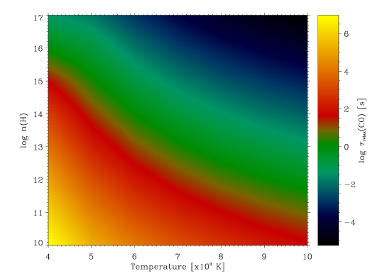
Figure 8: Relaxation time of the CO number density for a broad range of possible physical conditions in a stellar atmosphere. Note that the relaxation time increases when the temperature and/or hydrogen number density are reduced, while it decreases when the temperature and/or hydrogen number density are increased.

The linear analysis of the time evolution of the CO number density shows that CO is mainly driven by itself as dictated by Eq. (36). Therefore, it is possible to carry out a fit of this temporal evolution behavior and obtain a relaxation time $\tau_{\mathrm{relax}}$. Since a linear analysis is suitable for CO, the relaxation time can be calculated for a range of perturbations in the temperature and hydrogen number density. The results are shown in Fig. 8. The general trend is that, for a given density, the relaxation time is the larger the cooler the medium where the temperature perturbation is introduced. Similarly, for a given temperature of the unperturbed medium, the relaxation time increases rapidly with decreasing density. Short relaxation times are typical of high-temperature and high-density media (e.g. $t_{\rm relax}\,{\approx}\,0.006$ s for $n_{\rm H}=10^{16}\,{\rm cm}^{-3}$ and $T=6000$ K), while long relaxation times are characteristic of low-temperature and low-density situations (e.g. $t_{\rm relax}\,{\approx}\,400$ s for $n_{\rm H}=10^{14}\,{\rm cm}^{-3}$ and $T=4000$ K). This behavior can be easily understood in terms of the number of collisions per unit time, which decreases both when the temperature and/or the density decreases. In a realistic situation like in the solar atmosphere, one would find a broad range of relaxation times at a fixed atmospheric height because the existing rarefactions, compressions and temperature fluctuations are continually changing the physical conditions. Obviously, the situation is highly non-linear and the relaxation time concept, although useful, loses its meaning in the real Sun. Therefore, any firm conclusion needs to be achieved via detailed numerical simulations (see Asensio Ramos et al. 2003).

4 Concluding remarks

Thirty years ago, the total computational work ($W$) of the best available multilevel transfer codes scaled approximately as NP³, with NP the number of spatial grid points in a computational domain of fixed dimensions (e.g., Mihalas 1978). Twenty years ago, operator splitting methods based on Jacobi iteration were developed that yielded $W{\sim}{\rm NP}^{2}$ (e.g., Olson, Auer & Buchler 1986; Rybicki & Hummer 1991, 1992; Auer, Fabiani Bendicho & Trujillo Bueno 1994). Ten years ago, radiative transfer methods based on Gauss-Seidel and SOR iteration were developed for which $W{\sim}{\rm NP}{\,}\sqrt{{\rm NP}}$, which imply an-order-of-magnitude of improvement with respect to the MALI method (Trujillo Bueno & Fabiani Bendicho 1995; Trujillo Bueno & Manso Sainz 1999; Trujillo Bueno 2003). Such methods are also suitable for 2D and 3D radiative transfer applications because they do not require neither the construction nor the inversion of any non-local approximate $\Lambda$-operator (see the MUGA-3D code of Fabiani Bendicho & Trujillo Bueno 1999). Moreover, MUGA is the iterative method of choice for the development of the only multilevel RT method for which $W{\sim}{\rm NP}$ -that is, the non-linear multigrid method described by Fabiani Bendicho, Trujillo Bueno & Auer (1997).

In this article we have shown how the Multilevel Gauss-Seidel (MUGA) and Multilevel Successive Overrelaxation (MUSOR) methods can be applied for solving multilevel radiative transfer problems in spherical geometry, for both atomic and molecular lines. Our multilevel codes based on the MUGA and MUSOR methods offer a very powerful tool for the fast solution of realistic RT problems.