A New Multidimensional Relativistic Hydrodynamics code based on Semidiscrete Central and WENO schemes.

Abstract

We have proposed a new High Resolution Shock Capturing (HRSC) scheme for Special Relativistic Hydrodynamics (SRHD) based on the semidiscrete central Godunov-type schemes and a modified Weighted Essentially Non-oscillatory (WENO) data reconstruction algorithm. This is the first application of the semidiscrete central schemes with high order WENO data reconstruction to the SRHD equations. This method does not use a Riemann solver for flux computations and a number of one and two dimensional benchmark tests show that the algorithm is robust and comparable in accuracy to other SRHD codes.

1 Introduction

Gas flows at (ultra)relativistic speeds are an integral component of many astrophysical phenomena. Some significant examples of these include accretion disks around compact objects, Gamma ray bursts, collapse of (super)massive stars, pulsar wind nebula/supernova remnant interactions, Active Galactic Nuclei (AGN), X-ray binaries, superluminal jets and many others. As it stands, there is a massive amount of astronomical data from many of these sources that to date, have only been partially understood and which hold clues to many problems related to the phenomena mentioned above. Correlating these data with the theory in many of these phenomena would require doing simulations that would include modelling (ultra)relativistic gas/fluid flows. Such flows are described by non-linear hyperbolic conservation laws that have shock waves as possible solutions. Shock waves are difficult to approximate numerically using standard finite difference techniques as they usually lead to spurious oscillations. High Resolution Shock Capturing (HRSC) schemes are a class of numerical methods devoted specifically to approximating hyperbolic conservation laws. Over the past fifteen years HRSC research have progressed immensely and they have been applied to a wide variety of problems involving classical and relativistic hydrodynamics. For a pedagogical introduction to some modern HRSC schemes and their applications, see Levequque R. (2002); Toro (1999); Pen U. L. (2002). To date, the most commonly used HRSC schemes in relativistic hydrodynamics have been ones that have not incorporated many of the recent advances in HRSC research. In this work, we will apply a new scheme to the SRHD equations that is simpler than most of the previous approaches and incorporates a number of recent advances from HRSC research. In Rahman $\&$ Moore (2005), this scheme was applied to the multidimensional classical hydrodynamics code. The work presented here should be considered an extension of that work. Before describing the motivations behind the algorithm used in this work, we provide a brief review of numerical methods used for the SRHD equations and that of HRSC schemes.

Wilson J. R. (1972), Wilson et al. (1979), Hawley et al. (1984), and Centrella $\&$ Wilson (1984) were the first to apply numerical methods to approximate the SRHD equations. They discretized the SRHD equations using an explicit finite difference scheme with artificial viscosity and monotonic transport. Since their work, this technique has been used to study a number of astrophysical phenomena including stellar collapses, accretion disks, cosmology etc. Most SRHD schemes up to the late eighties used the artificial viscosity technique of Wilson et al. (1979) to handle shock waves. However, a major breakthrough occurred when HRSC schemes were applied to the SRHD equations (Martì et al. (1991); Marquina et. al (1992); Eulderink, F (1993, 1995)). One of the most significant of these new schemes was the relativistic Piecewise Parabolic Method (PPM) by Martí $\&$ Müller (1996) (MM) which was based on the PPM reconstruction scheme of Colella $\&$ Woodward (1985). For a recent review of modern SRHD schemes, we refer the reader to Martí $\&$ Müller (2003).

The use of HRSC schemes for SRHD equations essentially shifted the paradigm for solving these equations from artificial viscosity based methods to this approach. Modern HRSC schemes are based on two conventional approaches for solving hyperbolic conservation laws. These are the so-called upwind (Harten A. (1983); Van Leer B. (1979); Roe P. L., (1981); Toro (1999)) and central methods (Lax & Friedrichs (1971); Lax P. (1954); Nessyahu & Tadmore (1990)). A common aspect of most modern HRSC-SRHD schemes is that they are solved using upwind schemes that use so-called Riemann solvers to approximate the solution. A drawback of using Riemann solvers is that they are computationally expensive and difficult to implement because they need computations of eigenvalues and eigenvectors of the flux matrix and uses flux splittings etc., to compute the numerical fluxes. On the other hand, central schemes do not use Riemann solvers and are simpler and easier to implement. Until recently, central schemes were not considered for wide ranging applications because a trade-off for their simplicity was loss of accuracy. This is because central schemes were generally more dissipative than their upwind counterparts. However, recent progress in HRSC research has addressed this issue and some newer formulations of central schemes have been shown to be comparable performance-wise to the upwind approach. The work presented here is based on some of these newer central schemes. Before discussing them, we provide below a brief overview of central schemes and discuss the most important aspect of HRSC schemes known as non-oscillatory data reconstructions methods.

Modern central schemes are based on the first and second order shock capturing algorithms developed by Lax-Friedrichs (LxF) (Lax & Friedrichs (1971); Lax P. (1954)), and Nessyahu $\&$ Tadmore (1990) (NT), respectively. Since NT, there have been a number of extensions of central HRSC schemes to higher orders and multidimensions. Some of these recent extensions are summarized below. The NT scheme was extended to 3^rd order by Liu $\&$ Tadmor (1998), and to multidimensions by Jiang $\&$ Tadmore (1998). These were followed by a new formulation of central HRSC schemes known as semidiscrete central schemes. The semidiscrete schemes were designed to address the dissipation issue mentioned above and were proposed in Kurganov $\&$ Tadmore (2000) (KT). KT showed that semidiscrete schemes, which are formulated on non-staggered grids and use more accurate information of local speeds of propagation, are less dissipative than their staggered grid counterparts. Hence, these schemes retained the simplicity of the central approach and were comparable in accuracy to other Riemann solver based upwind approaches. The inception of semidiscrete central schemes precipitated a great deal research on extending this formalism which included higher order formulations in multidimensions, genuinely multidimensional formulations and unstructured grid formulations among others(Liu & Tadmore (1998); Jiang & Tadmore (1998); Levy et al. (2000, 2002); Kurganov &Petrova (2001); Kurganov & Noelle (2001); Kurganov & Levy (2000)).

Besides the method used to advance the solution, another aspect of HRSC schemes that is equally important for any algorithm is the so called non-oscillatory data interpolation method. Data interpolation is used in all HRSC schemes. Non-oscillatory data reconstruction is the piecewise continuous polynomial interpolation of the data (which may contain discontinuities) over the computational domain. Most of the HRSC schemes mentioned above use the so called Essentially Non-Oscillatory (ENO) (Harten et al. (1987)) data reconstruction algorithm for data interpolation. This methods works by interpolating the data using the smoothest stencil from a number of choices. A modern extension of ENO schemes is the Weighted Essentially Non-Oscillatory data reconstruction (WENO) algorithm (Liu et al. (1994); Jiang G-S, Shu C-W (1996)) that has a number of advantages over its predecessor. In order to take advantage of the developments in central approaches and high order data reconstruction, another class of HRSC schemes were developed as an extension of the NT scheme by Levy et al. (Levy et al. (2000, 2002)) called the Central Weighted Non-Oscillatory (CWENO) schemes. Recently, Kurganov $\&$ Levy (2000) (KL) have combined the semidiscrete central schemes with the WENO reconstruction method and proposed yet another, better HRSC scheme. The work presented here is based on the KL HRSC scheme which we will describe below.

Despite the many advances mentioned above, there have been relatively few attempts at applying central-type methods to computational astrophysics. However this is rapidly changing. Among the most significant attempts to apply central schemes for computational astrophysics, the following are noteworthy. Del Zanna $\&$ Bucciantini (2002), have developed an algorithm that is a variation of the conventional finite volume central type approach and applied it to multidimensional SRHD and SRMHD equations. They have also used these codes to study Pulsar Wind Nebula (PWN) interactions with the interstellar medium Del Zanna & Bucciantini (2004) and supernova remnants Del Zanna & Bucciantini (2003). Anninos $\&$ Fragile (2003,2004) have developed a new central type scheme for relativistic hydrodynamics in fixed, curved spacetime and have applied their scheme to study accretion disks around kerr black holes. Lucas-Serano et al. (2004) have assessed the applicability of central schemes to SRHD equations using the PPM data reconstruction scheme Colella & Woodward (1985). Their results were the first to demonstrate that central type schemes of KT can be used for SRHD. Recently, Shibata $\&$ Font (2005) have successfully tested the suitability of central type schemes for general relativistic simulations. We turn our attention now to applications of the WENO data reconstruction methods in computational astrophysics. Balsara (Balsara D. (2001)) have used the WENO methods extensively in magnetohydrodynamics. Feng et al. (2004), have recently developed a cosmological hydrodynamics code using the WENO reconstruction scheme. Zhang $\&$ MacFadyen (2005), have recently used the WENO scheme in their adaptive SRHD code. The work mentioned above point to a promising future for the application of central and WENO schemes in astrophysical hydrodynamics. Indeed, the work presented here was done concurrently with many of the recent work mentioned above. However, the algorithm presented here is the first to combine the WENO and the semidiscrete central approach for applications in SRHD. We describe below this algorithm and its novel aspects.

In a previous paper, Rahman $\&$ Moore (2005), we have described in detail the incentive behind our algorithm for multidimensional classical hydrodynamics. Many of the same reasons apply for the SRHD equations as well. The algorithm is based on combining the semidiscrete approach of Kurganov $\&$ Levy (2000) with high order WENO data reconstruction methods. To ensure robustness we have added the flattening, steepening and monotonicity preserving techniques of the PPM reconstruction scheme by Colella $\&$ Woodward (1985) to the data reconstruction scheme. Essentially, the simplicity of central schemes, the accuracy WENO reconstructions and the robustness of the piecewise parabolic method have been combined to propose a new robust central scheme. Building on the success of this algorithm for classical hydrodynamics, it has been applied to the SRHD equations. This work is original in several respects. It is the first attempt at solving the SRHD equations using the semidiscrete central scheme with WENO data reconstructions. The algorithm has been tested using both 3^rd. and 4^th. order data reconstruction techniques. It is also a dimensionally unsplit algorithm and to our knowledge is the only unsplit multidimensional algorithm in SRHD. The work presented here can be considered as laying the foundation for the development of a multi-purpose, multi-dimensional SRHD code that could be used to study a wide variety of astrophysical phenomena.

The paper is organized as follows. Sec. 2 presents the SRHD equations. Sec. 3 describes the new algorithm for numerically approximating the SRHD equations. In Sec. 4, we present the results of a number of one dimensional benchmark tests. In Sec. 5, the two dimensional tests are presented. Finally we conclude this paper in Sec. 6.

2 Relativistic Hydrodynamic Equations

As a system of hyperbolic conservation laws, the equations of special relativistic hydrodynamics are given by

$$\frac{\partial{\bf U}({\bf w})}{\partial t}+\frac{\partial{\bf f}^{i}({\bf w})}{\partial x^{i}}=0\quad.$$ (1)

where the indices run from 1 to 3. In the above equations ${\bf U}$ and ${\bf f}^{i}$ are given by

$${\bf U}({\bf w}) = (D\quad,S^{1}\quad,S^{2}\quad,S^{3}\quad,\tau)\quad,$$ (2)

$${\bf f}^{i}({\bf w}) = (Dv^{i}\quad,S^{j}v^{i}+p\delta^{ij}\quad,S^{i}-Dv^{i})\quad.$$ (3)

Here $\delta^{ij}$ is the Kronecker delta, $v^{i}$ is the three velocity and $p$ is the pressure. The relationship between the conserved variable and the primitive variable is given by

$$D = \rho W\quad,$$ (4)

$$S^{i} = \rho hW^{2}v^{i}\quad,$$ (5)

$$\tau = \rho hW^{2}-p-D\quad,$$ (6)

where $h$ is the specific enthalpy; $h=1+\varepsilon+p/\rho$, and $W$ is the Lorentz factor satisfying $W\equiv u^{0}=1/\sqrt{1-v^{2}}$ with $v^{2}=v^{i}v_{i}$. The 3-velocity components are obtained from the spatial components of the 4-velocity as $v^{i}={u^{i}}/{u^{0}}$. The equations above are closed by the ideal gas Equation of State (EOS) given by,

$$p=(\gamma-1)\rho\epsilon\quad,$$ (7)

where $\gamma$ is the adiabatic index of the ideal gas and $\epsilon$ the energy density. The difference between the conserved and the primitive variables in these equations require special treatment in the algorithm which will be discussed below.

3 The Semidiscrete Central WENO Algorithm for SRHD

This section presents the new algorithm for solving the SRHD equations implemented in this work. This algorithm is very similar to that presented in a previous paper (rahman05). Besides one major sub-step, that of recovering the primitive variables from the conserved variables, it is in fact identical. However, for the sake of completeness, a very brief description of it is provided.

As mentioned before, this new SRHD algorithm is based on the combination of the Semidiscrete Central scheme of Kurganov $\&$ Levy (2000) (KL), and the steepening, flattening and monotonicity preserving algorithm of MM. For a review and details of the derivation of KL, see Kurganov & Levy (2000). The reader is also referred to MM for details of the steepening, flattening and monotonicity preservation algorithms. In KL, the solution of a scalar hyperbolic conservation law in one dimension,

$$u_{t}+\frac{\partial f(u)}{\partial x}=0\quad$$

$$u(x,t=t^{n})=u^{n}(x)\quad,$$ (8)

is given by

$$\frac{d}{dt}\overline{u}_{j}(t)=-\frac{H_{i+\frac{1}{2}}(t)-H_{i+\frac{1}{2}}(t)}{\Delta x}\quad,$$ (9)

where the flux $H_{i+\frac{1}{2}}$ is,

$$H_{i+\frac{1}{2}}(t):=\frac{f(u^{+}_{i+\frac{1}{2}}(t))+f(u^{-}_{i+\frac{1}{2}}(t))}{2}-$$

$$\frac{a_{i+\frac{1}{2}}(t)}{2}\left[u^{+}_{i+\frac{1}{2}}-u^{-}_{i+\frac{1}{2}}\right]\quad.$$ (10)

$u^{+}_{i+\frac{1}{2}}$, $a_{i+\frac{1}{2}}$ are given by

$$u^{-}_{i+\frac{1}{2}}=P_{j}^{n}(x_{j+1/2})\quad,$$ (11)

$$a_{i+\frac{1}{2}}:=\max\{\rho(\frac{\partial f}{\partial u}(u_{j+1/2}^{-})),\rho(\frac{\partial f}{\partial u}(u_{j+1/2}^{+}))\}\quad,$$ (12)

where $\{P_{j}^{n}(x)\}$ is a non-oscillatory piecewise polynomial reconstruction of cell averaged data at time $t=t^{n}$, $\{\overline{u}_{j}^{n}(x)\}$. In this paper, both 3^rd. and 4^th order WENO reconstruction methods of Kurganov & Levy (2000); Levy et al. (2000) are used. In Eq. 10, $a_{i+\frac{1}{2}}$ is the speed of propagation of $u$ at the interface of a cell that is determined from the spectral radius of the Jacobian of the flux $f$. For a system of equations in multidimensions, the scheme given above can be extended as follows. A dimensionally unsplit approach can be used to extend Eq. 9 to multidimensions. In this approach, Eq. 9 is modified by adding another term corresponding to the flux differences in the y-direction. For a system of equations, the scalar $f$ is replaced by a vector ${\bf F}$ and $\frac{\partial f}{\partial u}$ is replaced by the Jacobian of ${\bf F}$.

For all the computations presented here, the piecewise polynomial interpolations have been done on the primitive variables from which the conserved variables are computed using Eqns. 4-6. In each step of our integration routine, once the conserved variables are updated, the primitive variables are immediately recovered. The method used to do this is by solving of a non-linear equation using the Newton-Raphson root finding method (see Martì $\&$ Müller (2003) for details). It is this aspect of numerical SRHD that makes them computationally more expensive than the Euler equations of gas dynamics. We can now summarize our algorithm in the following few steps:

step 1: Given initial data ${\bf{\overline{u}}_{j}^{n}}$ (primitive variables), use an $nth.$ (for n $\leq$ 4) order WENO reconstruction algorithm to construct a piecewise polynomial interpolation of each variable.

step 2: Apply the steepening (only to the density $\rho$), flattening and monotonicity preserving algorithms to the interface values of the primitive variables.

step 3: Update ${\overline{u}}_{j}^{n}$ (the conserved variables) to ${\overline{u}}_{j}^{n+1}$ using Eqns. 9 and 10 above.

step 4: Recover the primitive variables from the updated conserved variables.

step 5: Repeat steps 1 to step 4

The time integration of Eq. 9 is done using a high order total variation diminishing (TVD) Runge-Kutta scheme Shu & Osher (1988), which combines the first order forward Euler method with predictor-corrector steps. This is,

$$U^{(1)}=U^{n}+\Delta TL(U^{n})$$

$$U^{(2)}=\frac{3}{4}U^{n}+\frac{1}{4}U^{(1)}+\frac{3}{4}\Delta tL(U^{(1)})$$

$$U^{n+1}=\frac{1}{3}U^{n}+\frac{2}{3}U^{(2)}+\frac{2}{3}\Delta tL(U^{(2)})\quad.$$ (13)

4 Numerical Tests

SRHD schemes are usually tested by a series of standard benchmark problems. The most important of these are the so-called $shock$ $tube$ Riemann problems. A shock tube test in one dimension can be described as follows; a one dimensional pipe is divided into two halves by a membrane and the thermodynamic states of each half is specified. When the membrane between the halves is removed, depending on the initial conditions, contact discontinuities, shocks and rarefaction waves etc. will result. Analytic solutions of the amplitude and position of these features have been derived for both classical and relativistic hydrodynamics. For analytical solutions of the relativistic hydrodynamics shock tube problems, see Martì $\&$ Müller (1994); Thompson (1986); Pons et al. (2000). For a list of some standard shock tube tests along a review of the performance of some SRHD schemes, see Martí $\&$ Müller (2003). In addition to the Riemann problems, we have done some other tests that do not have analytic solutions. In each case, the results are compared to the literature.

In the following two sections, we present the results of the benchmark tests in one and two dimensions. Before we present our results, we list in Table 1, the input parameters we have used in the tests for contact steepening, flattening and the monotonicity preserving steps. We have set $\gamma=5/3$ in all the computations, unless otherwise specified.

4.1 One Dimensional tests

Problem 1:

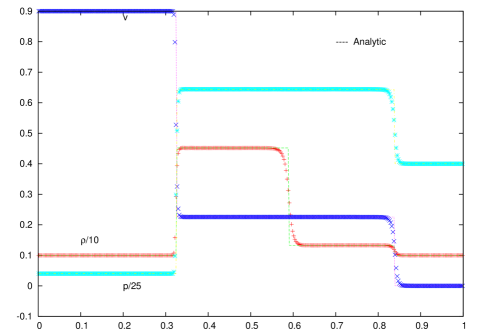
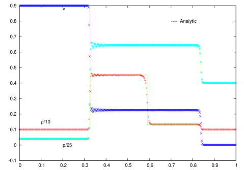
Figure 1: Density, Pressure and velocity profiles for test 1 (Sec. 5.1) at t=0.4 using 3^rd (top) and 4^th (bottom) order WENO reconstructions and n=400.

The initial states of the right and left halves of the domain are given by $p_{\rm L}=1.0,\rho_{\rm L}=1.0,v_{\rm L}=0.9$ (left) and $p_{\rm R}=10.0,\rho_{\rm R}=1.0,v_{\rm R}=0$ (right). This initial condition leads to a strong reverse shock. In Figure 1, the results are shown for both 3^rd and 4^th order reconstructions. We have shown the density, velocity and pressure profiles at t=0.4 and compared the numerical results to analytic solutions. Excellent agreement between these results and the analytic solutions is noted. Also, these results match closely with those obtained by Lucas-Serano et al. (2004) which were obtained using the PPM. As was the case in Lucas-Serano et al. (2004), small oscillations noted behind the shocks disappear completely as the CFL number is lowered. However, such oscillations remain more pronounced for the 4^th order reconstruction. In Table 2, $L^{1}$ errors for the density for both 3^rd and 4^th order reconstructions are shown. It shows that the order of the scheme is approximately one, as is expected for solutions with shocks.

Problem 2:

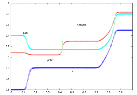
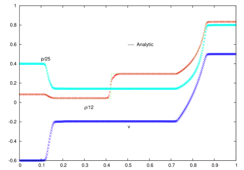
Figure 2: Density, Pressure and velocity profiles for test 2 (Sec. 5.1) at t=0.4 using 3^rd (top) and 4^th (bottom) order WENO reconstructions and n=400.

The initial states of the right and left halves of the domain are $p_{\rm L}=10.0,\rho_{\rm L}=1.0,v_{\rm L}=-0.6$ (left) and $p_{\rm R}=10.0,\rho_{\rm R}=1.0,v_{\rm R}=0.5$ (right). In Figure 2, the results using the 3^rd and 4^th order WENO reconstructions are presented. Once again, we note that the shock positions and velocities are captured well by both reconstruction schemes. Unlike the previous test, post shock oscillations are not seen in either of the reconstructions. Direct comparison with Lucas-Serano et al. (2004), show good agreements as well. Table 3 presents the $L^{1}$ errors of the density for both 3^rd and 4^th order reconstructions. The order is approximately one for both cases except for very high grid spacings.

Problem 3:

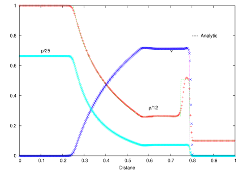
Figure 3: Density, Pressure and velocity profiles for test 3 (Sec. 5.1) at t=0.35 using 3^rd (top) and 4^th (bottom) order WENO reconstructions and n=400.

The initial states of the right and left handed halves of the domain are given by $p_{\rm L}=13.3,\rho_{\rm L}=10.0,v_{\rm L}=0$ (left) and $p_{\rm R}=0,\rho_{\rm R}=1.0,v_{\rm R}=0$ (right). We expect a shock wave, a contact discontinuity and a rarefaction wave from this test. Figure 3 shows the results of the computation. There is good agreement between the computed and analytic solutions. Direct comparison with Lucas-Serano et al. (2004) and Zhang $\&$ MacFadyen (2005) show good agreements as well. In Table 4, the $L^{1}$ errors of the density for both for 3^rd and 4^th order reconstructions are shown. Although irregular, these values show similar trends and magnitudes to those obtained by others (see Lucas-Serano et al. (2004), Zhang $\&$ MacFadyen (2005)). We believe the error could be optimized by appropriately fine tuning the smoothing and flattening parameters.

Problem 4:

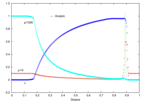
Figure 4: Density, Pressure and velocity profiles for test 4 (Sec. 5.1) at t=0.4 using 3^rd (top) and 4^th (bottom) order WENO reconstructions and n=400.

The initial states of the right and left handed halves of the domain are given by $p_{\rm L}=1000.0,\rho_{\rm L}=1.0,v_{\rm L}=0$ (left) and $p_{\rm R}=0.01,\rho_{\rm R}=1.0,v_{\rm R}=0$ (right). The initial condition gives rise to a right-moving shock, a left-moving rarefaction wave and a contact discontinuity in between. This is a fairly demanding test due to the $10^{5}$ order pressure ratio. In Figure 4, we show the results of our computation. As expected the 3^rd order scheme is more dissipative than the 4^th order scheme. Once again, a direct comparison between the results and analytic solutions show comparable agreements to the same tests done with other schemes (see Lucas-Serano et al. (2004), MacFadyen and Zhang (2005)). The $L^{1}$ errors (Table 5) of the density also show similar results.

Problem 5 (Shock Reflection Test) We consider now an even more severe test for the scheme. The shock reflection test consists of an ultra-cold relativistic wind hitting a solid wall and a reflected shock wave propagating backward leaving a static region of hot gas. The Lorenz factor of the wind is set by the precision level of the code. Hence, winds at very high speeds are considered. To directly compare our results with that of Del Zanna $\&$ Bucciantini (2002), Lucas-Serano et al. (2004), and Zhang $\&$ MacFadyen (2005), we have chosen the following initial conditions; $p=.01,\rho=1.0,v=0.99999,v=0.9999999999$ for the first and second tests, respectively. The solid wall is placed at the right edge of the computational domain. The post shock density is an increasing function of the initial flow velocity. The compression ratio $\sigma=\rho_{2}/\rho_{1}$, satisfies

$$\sigma=\frac{\gamma+1}{\gamma-1}+\frac{\gamma}{\gamma-1}\epsilon_{2}$$ (14)

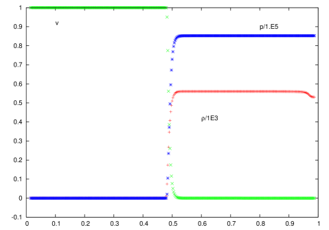
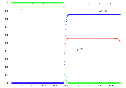
Figure 5: Density, Pressure and velocity profiles for test 5 (Sec. 5.1), v= .99999 using 3^rd (top) and 4^th (bottom) order WENO reconstructions and n=400.

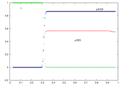
Figure 6: Density, Pressure and velocity profiles for test 5 (Sec. 5.1), v= .9999999999 using 3^rd (top) and 4^th (bottom) order WENO reconstructions and n=400.

where, $\epsilon_{2}=W_{1}-1$ and $W_{1}$ is the initial Lorentz factor. We have used $\gamma=4/3$ for this test. The results are shown in Figures 5 and 6. Consider first Figure 5, which corresponds to a Lorenz boost factor, $W=224$. Direct comparison between our results and those of Lucas-Serano et al. (2004), and Del Zanna $\&$ Bucciantini (2002), show good qualitative agreement. Note that both 3^rd and 4^th order reconstruction schemes capture the shock wave without oscillations, in contrast to the case of Del Zanna and Bucciantini (2002), where the 3^rd order CENO scheme fails. Next, consider the case of $W=70710.675$ (Figure 6). Comparing our results to those of Zhang $\&$ MacFadyen (2005), there is excellent qualitative agreement. These results show that the scheme is robust against both 3^rd and 4^th order reconstructions for ultra-relativistic flows.

Problem 6: Mixed Solution test

For the final one dimensional test, we followed Del Zanna and Bucciantini (2002), and considered a test in which oscillatory and smooth solutions arise close together simultaneously. The initial configuration is given by;

$$p_{L}=50.0,\rho_{L}=5.0,\qquad v_{L}=0(\rm{left})\quad,$$ (15)

$$p_{R}=5.0,\rho_{R}=2.0+0.3\sin 50x,\qquad v_{R}=0(\rm{right})\quad.$$ (16)

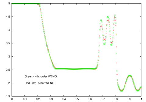
Figure 7: Mixed soulution test (test 5, Sec. 5.1) for 3^rd and 4^th order WENO reconstruction at t= .36. Shown ar the density profiles.

The solution consists of the interaction between a blast wave and a density wave. The results are shown in Figure 7, which shows the density profile for both the 3^rd and 4^th order reconstructions simultaneously. We see that the 4^th order scheme gives more oscillatory results than 3^rd order WENO. Direct comparison with Del Zanna $\&$ Bucciantini (2002), show good agreement.

5 2-dimensional Relativistic Hydrodynamics

The one dimensional scheme is extended to two dimensions in a straightforward manner using a dimensionally unsplit scheme for advancing the solution that was described earlier. The two dimensional reconstruction is done using dimensional splitting. For the multidimensional tests, we consider the a two dimensional Riemann problem, a symmetric blast wave and a relativistic jet. All of these tests are compared to previous results.

5.1 Two-dimensional shock tube test

Following Del Zanna $\&$ Bucciantini (2002), Lucas-Serano et al. (2004), and Zhang and MacFadyen (2005), consider the following two-dimensional Riemann Problem. A two dimensional square region is divided into four quadrants and the initial conditions given by

$$(\rho,v_{x},v_{y},p)^{NE}= (0.1,0.0,0.0,0.01)\quad,$$

$$(\rho,v_{x},v_{y},p)^{NW}= (0.1,0.99,0.0,1.0)\quad,$$

$$(\rho,v_{x},v_{y},p)^{SW}= (0.5,0.0,0.0,1.0)\quad,$$

$$(\rho,v_{x},v_{y},p)^{SE}= (0.1,0.0,0.99,1.0)\quad.$$ (17)

Outflow boundary conditions are used throughout the domain and the adiabatic gas index is set to $\gamma$ = 5/3. The resulting pattern is shown in Figure 8 which were computed using the 4^th order WENO and PPM (from Lucas-Serano et al. (2004)) reconstruction schemes. The solutions are shown at time time $t=0.4$. The PPM based calculations have been presented here for the sake of direct comparison. The salient features of these results are as follows. Note that the WENO based scheme gives sharper contact discontinuities than the PPM scheme for the same grid resolution. Around the head of the shock, we have been able to resolve both the bow shock and the inner shock structure. Around the tails, where the shock merge, we are able resolve the jet-like structure seen due to the merging of the two discontinuities.

5.2 Spherically symmetric blast-wave test

In this test, a cylindrically symmetric blast wave is studied. The set-up of the problem is as follows. The domain is $[-1,1]\times[-1,1]$ with outflow boundary conditions. The initial configuration is given by

$$(\rho,v_{x},v_{y},p)=(1.,0.,0.,1000.)\quad{\rm if}\qquad r^{2}\quad<\quad(.4)^{2}$$

$$(\rho,v_{x},v_{y},p)=(1.,0.,0.,1.0)\quad{\rm Otherwise}\quad.$$ (18)

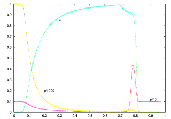
Figure 9: Cylindrically symmetric blast wave (Sec. 6.2) using 4^th order WENO. Solution at t=0.4 and n=250. Solid lines represent one dimensional calculations.

This problem does not have an analytic solution so the results are compared to a one dimensional simulation. The results are also compared to Del Zanna $\&$ Bucciantini (2002), and Zhang $\&$ MacFadyen (2005). The initial condition given above give rise to a cylindrically symmetric blast wave moving outward, a rarefaction wave moving inward and and a contact discontinuity. A 4^th order WENO data reconstruction algorithm was used for this test. In Fig. 9, the test results are shown at time $t=0.4$. Direct comparison with the above mentioned references show excellent agreement. Cylindrical symmetry is also well preserved in the computations.

5.3 2D Relativistic Jet

The final multidimensional test undertaken for our algorithm is that of relativistic jets in planar geometry. The dynamics and morphology of jets have been studied by many authors (see Zhang $\&$ MacFadyen (2005), and references therein). This is a standard benchmark for testing any new relativistic HRSC scheme. To test the ability of our codes to capture the salient features of relativistic jets, we have considered the following scenario. Our tests are done in planar geometry. We consider a rectangular domain of length $[0,45]\times[-25,25]$. Through a small opening along the axis of symmetry we inject a relativistic fluid at $v_{x}=0.99c,V_{y}=0.0$. The pressure between the inflow and the ambient medium is considered to be at equilibrium. And we take a density ratio of the inflow and ambient medium of $0.01$. Reflective boundary conditions are used along the axis-of symmetry. Otherwise outflow boundary conditions are used elsewhere.

Figs. 10-11 progression of the jets at times $t=5$, $t=25$, $t=50$ and $t=75$ respectively. Comparing our results to Lucas-Serano (2004), Del Zanna $\&$ Bucciantini (2002), and Zhang $\&$ MacFadyen (2005), we find good qualitative agreement. The jets capture the expected morphology quite well. There is a supersonic jet that extends from the nozzle and impacts with the ambient medium, at which point we note a terminal planar shock, a contact discontinuity and a bow shock. There is a cocoon that separates the ambient medium from the jet material by a contact discontinuity where we note Kelvin-Helmholtz instabilities. We also note the absence of $carbunckles$, that is purely a numerical artifact.

Figs. 12-13, show snapshots of the same calculations using a slightly narrower opening of the in flowing jets. Compared to the previous case, the jets are more collimated in this case.

6 Summary and Conclusion

We have developed a new multidimensional relativistic hydrodynamics code based on the semidiscrete central and WENO reconstruction approach, and some elements of the PPM method. This is the first such multidimensional relativistic code combining these elements. A dimensionally unsplit scheme was used to advance the solution. We also carried out a number of one and two dimensional tests of the code using both 3^rd and 4^th order reconstruction methods. The test results are comparable to a number of other codes currently being used in computational astrophysics. In all cases, the tests showed good agreements with codes currently in use.

The work presented here should be considered as the first few steps towards the development of a multi-purpose relativistic hydrodynamics code. Some of the developments mentioned above on semidiscrete central schemes could well extend the performance of our code. These include the genuinely multidimensional formulation, the formulation on unstructured grid or higher order WENO reconstructions. From the point of applications, we are working to extend our code to three dimensions, provide it with adaptive capabilities and apply it for parallel architecture using MPI.

Test	$K_{0}$	$\eta^{(1)}$	$\eta^{(2)}$	$\epsilon^{(1)}$	$\omega^{(1)}$	$\omega^{(2)}$	$\epsilon^{(2)}$
Test 1	1.0	5.0	0.05	0.7	0.52	10.0	5.
Test 2	1.0	5.0	0.05	0.7	0.52	10.0	5.0
Test 3	1.0	5.0	0.05	0.7	0.52	10.0	5.0
Test 4	1.0	5.0	0.05	0.7	0.52	10.0	5.0
Test 5	1.0	5.0	0.1	0.1	0.52	10.0	0.0001

Table 1: Values of the flattening, steepening and monotonicity preserving parameters used in one dimensional shock tube tests presented in Sec. 5.1

N	$L^{1}$-error (4th order)	Rate	$L^{1}$-error (3rd order)	Rate
40	2.82E-1	-	3.17E-1	-
80	1.33E-1	1.08	1.55E-1	1.06
160	6.77E-2	.9466	8.04E-2	0.96
320	3.4E-2	1.02	4.22E-2	0.94
640	1.75E-2	0.98	2.32E-2	0.92

Table 2: $L^{1}$ errors of density in Test 1, Sec. 5.1. Shown are the errors in density for both 3^rd and 4^th order reconstruction.

N	$L^{1}$-error (4th order)	Rate	$L^{1}$-error (3rd order)	Rate
40	2.53E-1	-	3.76E-1	-
80	1.66E-1	0.63	2.51E-1	0.61
160	7.31E-2	1.22	1.26E-1	0.99
320	3.77E-2	0.98	6.55E-2	0.95
640	1.92E-2	1.15	3.33E-2	0.99

Table 3: $L^{1}$ errors for Test 2, Sec. 5.1. Shown are the errors in density for both 3^rd and 4^th order reconstruction.

N	$L^{1}$-error (4th order)	Rate	$L^{1}$-error (3rd order)	Rate
40	4.40E-1	-	4.98E-1	-
80	2.28E-1	0.95	2.80E-1	0.84
160	1.30E-1	0.81	1.49E-1	0.92
320	6.19E-2	1.07	7.23E-2	1.04
640	3.23E-2	0.94	3.77E-2	0.94

Table 4: $L^{1}$ errors for Test 3, Sec. 5.1. Shown are the errors in density for both 3^rd and 4^th order reconstruction.

N	$L^{1}$-error (4th order)	Rate	$L^{1}$-error (3rd order)	Rate
80	2.79E-1	-	2.81E-1	-
160	1.85E-1	0.51	1.85E-1	0.6
320	1.51E-1	0.29	1.50E-1	0.3
640	1.01E-1	0.57	9.42E-2	0.66

Table 5: $L^{1}$ errors for Test 3, Sec. 5.1. Shown are the errors in density for both 3^rd and 4^th order reconstruction.

Figure 8: 2D Riemann problem, (Sec. 6.1). Logarithmic density plots are shown using our scheme (top) using the 4^th order WENO schme and that using the PPM reconstruction method (bottom) of Lucas-Serano et al. (2004). Solution showm at t=0.4 and n=400

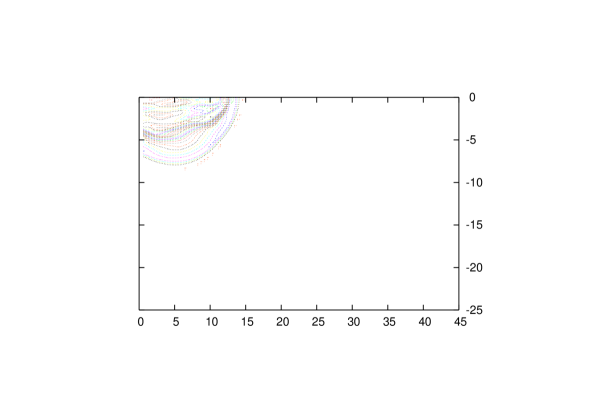
Figure 10: Two dimensional jet problem (Sec. 6.3). Density profile at t=5 (top), t=25 (bottom)

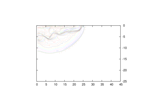
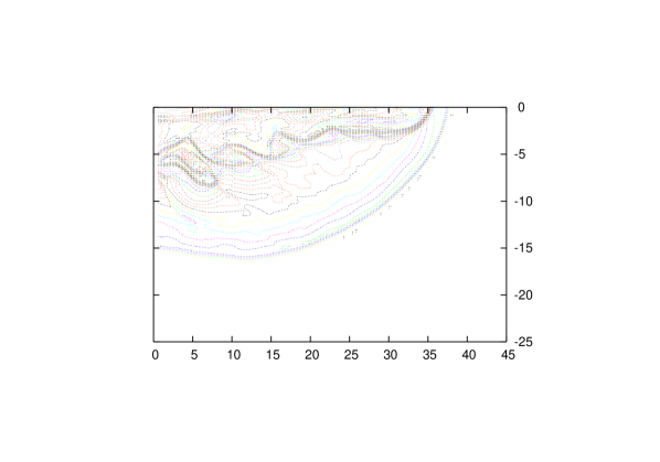
Figure 11: Two dimensional jet problem (Sec. 6.3). Density profile at t=50 (top), t=70 (bottom)

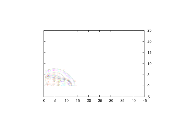
Figure 12: Two dimensional jet problem (Sec. 6.6.3). Density profile at t=5 (top), t=25 (bottom)

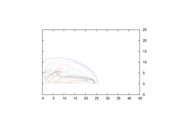
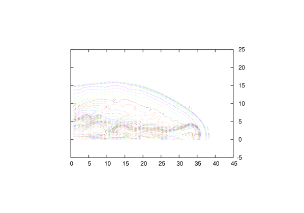
Figure 13: Two dimensional jet problem (Sec. 6.3). Density profile at t=50 (top), t=70 (bottom)

References

- Aloy et al. (1999) Aloy M.A., Ibànez J. M., Martí J. M., Müller E., ApJS, 122, 151 (1999).
- Anninos P. & Fragile C. (2003) Anninos P., Fragile C., ApJS, 144, 243 (2003).
- Anninos P. & Fragile C. (2004) Anninos P., Fragile C., astro-ph/0403356.
- Balsara D. (2001) Balsara D., , 174, 614 (2001).
- Centrella Wilson (1984) Centrella, J., and Wilson, J.R., ApJS, 54, 229 (1984).
- Colella & Woodward (1985) Colella P., Woodward P.R., , 45, 174 (1985).
- Del Zanna & Bucciantini (2003) Del Zanna L., Bucciantini N., astro-ph/0303491.
- Del Zanna & Bucciantini (2004) Del Zanna L., Bucciantini N., astro-ph/0412534.
- Eulderink, F (1993) Eulderink, F., Numerical Relativistic Hydrodynamics, PhD Thesis, (Rijksuniverteit te Leiden, Leiden, Netherlands, 1993).
- Eulderink, F (1995) Eulderink, F., and Mellema, G., Astron. Astrophys. Suppl., 110, 587, (1995).
- Feng L. et al. (2004) Feng L. et al., ApJ, 612, 1 (2004).
- Lax & Friedrichs (1971) Friedrichs K.O., Lax P.D., Pro. Nat. Acad. Sci. U.S.A., 68, 1686 (1971).
- Harten A. (1983) Harten A., , 49, 357 (1983).
- Harten et al. (1987) Harten A., Engquist B., Osher S., Chakravarthy S. R., , 71, 231 (1987).
- Hawley et al. (1984) Hawley, J. F., Smarr, L. L., Wilson, J. R., ApJS, 55, 211 (1984).
- Jiang & Tadmore (1998) Jiang G.-S., Tadmore E., , 19, 1892 (1998).
- Jiang G-S, Shu C-W (1996) Jiang G-S, Shu C-W, , 126, 202 (1996).
- Kurganov & Levy (2000) Kurganov A., Levy D., , 22, 4, 1461 (2000).
- Kurganov & Tadmore (2000) Kurganov A., Tadmore E., , 160, 241 (2000).
- Kurganov & Tadmore (2002) Kurganov A., Tadmore E., Numerical Methods for Partial Differential Equations 18, 608 (2002).
- Kurganov &Petrova (2001) Kurganov A., Petrova G., Numer. math., 88, 4, 683 (2001).
- Kurganov & Noelle (2001) Kurganov A., Noelle S., Petrova G., , 23, 3, 707 (2001).
- Kurganov A., Petrova G. (2005) Kurganov A., Petrova G., Numerical Methods for Partial Differential Equations, 21, 536 (2005).
- Lax P. (1954) Lax P. D., Comm. Pure and Applied. Mathematics 7, 154 (1954).
- Levequque R. (2002) LeVeque R., Finite Volume Methods for Hyperbolic Problems, Cambridge Texts in Applied Mathematics, Cambridge University Press, Cambridge. (2002).
- Levy et al. (2000) Levy D., Puppo G., Russo G., , 22, 2, 656 (2000).
- Levy et al. (2002) Levy D., Puppo G., Russo G., , 24, 2, 480 (2002).
- Liu et al. (1994) Liu L., Osher S, Chan T., 115, 200 (1994).
- Liu & Tadmore (1998) Liu L., Tadmore E., Numer. Math., 79, 4, 397 (1998).
- Lucas Serano et al. (2004) Lucas Serano et al. astro-ph/0407541.
- Marquina et. al (1992) Marquina et al., Astron. Astrophys., 258, 566 (1992).
- Martì et al. (1991) Martì J. M, Ibanez, J. M, Miralles, J. A., Phys. Rev. D, 43, 3794 (1991).
- Martì Müller (1994) Martì J., Müller E., J. Fluid Mech., 258, 317 (1994).
- Martì Müller (2003) Martì J., Müller, E., Living Reviews, 2003.
- Martì Müller (1996) Martì J., Müller E., J. Comput. Phys., 123, 1 (1996).
- Nessyahu & Tadmore (1990) Nessyahu H., Tadmore E., , 87, 408 (1990).
- Pen U. L. (2002) Pen U. L., astro-ph/0210611.
- Pons et al. (2000) Pons J. A., Martì J., Ml̈ler, E., J. Fluid Mech., 422, 125 (2000).
- Rahman Moore (2005) Rahman T., Moore R. B., A New Multidimensional Hydrodynamics code based on Semidiscrete Central and WENO schemes., astro-ph/0511728.
- Roe P. L., (1981) Roe P. L., , 43, 357, (1981).
- Shu & Osher (1988) Shu C.-W., Osher S. 77, 439 (1988).
- Thompson (1986) Thompson K. W., J. Fluid Mech., 171, 365 (1986).
- Toro (1999) Toro E. F., Riemann Solvers and Numerical Mmethods for fluid dynamics : A practical introduction., Berlin ; New York : Springer, 1999.
- Van Leer B. (1979) Van Leer B., , 32, 101 (1979).
- Wilson, J.R. (1972) Wilson J. R., ApJ, 173, 431 (1972).
- Wilson J. R. (1979) Wilson, J. R.,A Numerical Method for Relativistic Hydrodynamics, Smarr L. L., ed., Sources of Gravitational Radiation, 423-446, (Cambridge University Press, Cambridge, U.K., 1979).
- Zhang & MacFadyen (2005) Zhang W., MacFadyen A., astro-ph/0505481.