MHD simulations of radiative jets from young stellar objects:

We study the H$\alpha$ emission from jets using two-dimensional axisymmetrical simulations. We compare the emission obtained from hydrodynamic (HD) simulations with that obtained from magnetohydrodynamics (MHD) simulations. The magnetic field is supposed to be present in the jet only, and with a toroidal configuration. The simulations have time-dependent ejection velocities and different intensities for the initial magnetic field. The results show an increase in the H$\alpha$ emission along the jet for the magnetized cases with respect to the HD case. The increase in the emission is due to a better collimation of the jet in the MHD case, and to a small increase in the shock velocity. These results could have important implications for the interpretation of the observations of jets from young stellar objects.

1 Introduction

Collimated outflows are observed in a variety of astrophysical objects, with typical spatial scales ranging from $\sim 1$ pc for jets from young stellar objects (YSOs) up to several megaparsecs for extragalactic jets. All of these jets seem to be associated with accretion disks, which suggests the existence of a scale-independent physical mechanism responsible for the ejection and collimation of these outflows. The presently more accepted models are the magnetocentrifugal models (Blandford & Payne BP1982 (1982); Uchida & Shibata US1985 (1985)), in which the ejection is driven by the presence of a dynamically important magnetic field in the accretion disk-central object system, and the collimation of the jet is due to the toroidal component of the magnetic field, which is able to collimate the outflows by pinching forces. The toroidal magnetic field is generated by the twisting of the magnetic field due to the rotation of the system. The region where this process acts is too close to the central object to be resolved observationally, and one possible way to obtain some insight into this region is by studying the properties of the outflows.

In particular, a lot of progress has recently been made regarding observations of the outflows from YSOs (see the review by Reipurth & Bally RB2001 (2001)). The caracteristic spectral emission of these objects is believed to come from the region behind the shock, from recombination of the ionized gas (for the hydrogen lines) and electron excitation (and de-excitation) within ions (Schwartz S1975 (1975)), and the typical knot structure visible along the jet could be interpreted as due to a time-dependent ejection from the young stellar object (YSO) (Reipurth R1989 (1989); Raga et al.Ral1990 (1990)).

In the past few years, several authors have studied the effect of the magnetic field on the dynamical evolution of HH objects (e. g. O’Sullivan & Ray OR2000 (2000); Stone & Hardee SH2000 (2000); Cerqueira et al. Cal1997 (1997)). Frank et al. (Fal1999 (1999)) showed that ambipolar diffusion could be important to smear out the magnetic field ejected with the jets, but only on timescales comparable or larger than the dynamical timescales of the jets. The determination of a magnetic field in the outflows would represent a test for the magnetocentrifugal mechanism. In particular, the presence of a dynamically important toroidal component of the magnetic field would represent an indirect proof of this mechanism. However, direct observations of magnetic fields in jets are very difficult, and there is yet no clear observational determination of the magnetic field intensity in jets.

Several hydrodynamic (HD) simulations with calculations of the spectral emission of HH objects have been presented in the past (e. g. Blondin et al. Bal1990 (1990); Raga R1994 (1994)), but such calculations have never been published for the magnetized case. The simulations with magnetic fields have concentrated on the dynamical aspects and the evolution of the jet rather than on obtaining predictions of the emitted spectrum. These simulations usually include a radiative cooling rate (given, e.g., by the coronal cooling function of Dalgarno & McCray DM1972 (1972)), and different magnetic field configurations. The main features found in magnetized jets with respect to HD jets are the presence of a “nose cone”, better collimation, an increase in the density along the direction of propagation, and some effects on Kelvin-Helmoltz and Rayleigh-Taylor instabilities (resulting in changes in the leading bow shock, e. g. Todo el al Tal1993 (1993); Cerqueira & de Gouveia Dal Pino CD1999 (1999)).

With respect to the emitted spectrum, Hartigan, Morse & Raymond (Hal1994 (1994)) compared observed and predicted emission lines ratios (using plane-parallel shock models) to find an upper limit of 30 $\mu$G for the magnetic field of the jet. Cerqueira & de Gouveia Dal Pino (2001a ), using a semiempirical formula (valid for a shock velocity between $20$ and $80$ km s^-1) found the ratio between the H$\alpha$ emission of a magnetized and a non-magnetized jet. They obtained that the H$\alpha$ emission increases due to the presence of a magnetic field, and that the dominant cause of this increase is the toroidal component of the magnetic field.

Therefore, no direct calculation of the effect of the magnetic field on the emission from a jet has yet been made. Trying to fill this gap, we have carried out 2D, axisymmetric, MHD simulations of jets, looking for the differences in the predicted H$\alpha$ emission from magnetized jets with respect to the hydrodynamic case. The paper is organized as follows. In section 2, we explain in some detail the numerical algorithm that has been used, the initial conditions of the simulations and the approximations used to calculate the emission. In section 3 we summarize and discuss the results obtained, and in section 4 we draw our conclusions.

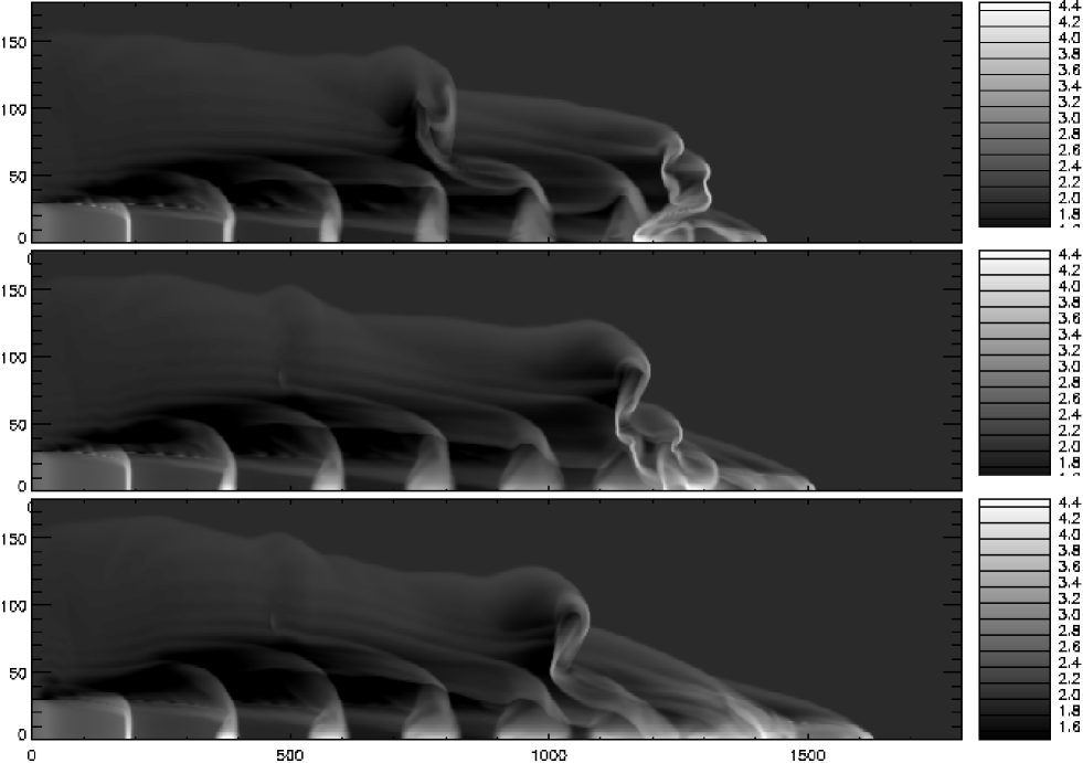
Figure 1: Numerical density for the models HD (hydrodynamic), weak MHD ($\beta=1$), and strong MHD ($\beta=0.4$), after a 500 yrs integration time. The right bar gives the logarithm of the numerical density (in cm^-3) The axes are labeles in pixels, and the displayed domain has a physical size of ($L_{z}$,$L_{r}$) = ($3\times 10^{17}$, $3\times 10^{16}$) cm. A pixel correspond to a physical size of $1.66\times 10^{14}$ cm.

2 Simulations

2.1 Numerical method

To study the H$\alpha$ emission from YSO jets, we have carried out a set of 2D, axysimmetrical simulations using a MHD code, modified to include the cooling and the evolution of the hydrogen ionization fraction. We solve the following set of equations:

$${\partial\rho\over\partial t}+\nabla\cdot(\rho\@vec{v})=0$$ (1)

$${\partial\rho\@vec{v}\over\partial t}+\nabla\cdot(\rho\@vec{v}\@vec{v}+p_{tot}I-\@vec{B}\@vec{B})=0$$ (2)

$${\partial e\over\partial t}+\nabla\cdot((e+p_{tot})\@vec{v}-(\@vec{v}\cdot\@vec{B})\@vec{B})=-n^{2}\Lambda$$ (3)

$${\partial\@vec{B}\over\partial t}+\nabla\cdot(\@vec{v}\@vec{B}-\@vec{B}\@vec{v})=0$$ (4)

$${\partial n_{H^{0}}\over\partial t}+\nabla\cdot(n_{H^{0}}\@vec{v})=n_{H^{+}}n_{e}\alpha(T)-n_{H^{0}}n_{e}C(T)$$ (5)

where $\rho$ is the mass density, $\@vec{v}$ is the velocity vector, $p_{tot}=p_{gas}+B^{2}/2$ is the (magnetic $+$ thermal) total pressure, $I$ is the identity matrix, $\@vec{B}$ is the magnetic field normalized with respect to $\sqrt{4\pi}$, $e$ is the total energy defined as $e=\frac{1}{\gamma-1}p_{gas}+\frac{1}{2}\rho v^{2}+\frac{1}{2}B^{2}$ (with $\gamma=5/3$), and finally $\Lambda$ is the cooling function. These equations represent the conservation of mass (1), momentum (2), energy (3) and magnetic flux (4). Eq. (5) represents the evolution of the hydrogen neutral fraction. This equation is coupled to the others by the cooling function $\Lambda$, which is a function of the ionization fraction. In Eq. (5):

$$\alpha(T)=2.55\cdot 10^{-13}(T/10^{4})^{-0.79}$$

$$C(T)=5.38\cdot 10^{-11}e^{-\frac{157828}{T}}/\sqrt{T}$$

are the recombination and collisional ionization coefficients (Cox C1970 (1970)), and $T$ is the gas temperature.

To solve this equation system, we use a second order upwind scheme, which integrates the MHD equations using a Godunov method with a Riemann solver. The Riemann problem is solved using primitive variables and the magnetic field divergence is maintained close to zero using the CT method (Toth T2000 (2000)). The algorithm is similar to the one of Falle, Komissarov and Joarder (Fal1998 (1998)), except that to preserve a small divergence of the magnetic field we use a constrained transport method. However, the magnetic field divergence is automatically equal to zero in all our axysimmetrical simulations because we use a toroidal magnetic field configuration. To treat correctly the source terms in cylindrical coordinates, these terms are averaged on the cell volume (see the discussion in the appendix of Falle F1991 (1991)). The code was tested with one- and two-dimensional tests (Ryu et al. Ral1995 (1995); Toth T2000 (2000); also see De Colle D2005 (2005)).

To solve Eq. (3), we first integrate the equation without the cooling term finding a new value for the energy $e^{\prime}$, and afterwards we use this new energy value to integrate the equation

$${\partial e^{\prime}\over\partial t}=-n^{2}\Lambda(T)=-n^{2}\Lambda_{0}{T\over T_{0}},$$ (6)

where $n$ is the number density (assumed to be constant within the timestep) and we approximate $\Lambda(T)$ in a locally linear form. This equation has an exact solution for the gas pressure:

$$p_{gas}=p_{0,gas}e^{-2\Lambda_{0}n_{H}\Delta t/3k_{B}T}.$$ (7)

where $n_{H}$ is the total (ionized more neutral) hydrogen density, $T$ is the gas temperature, $k_{B}$ is the Boltzmann constant and $\Delta t$ is the time step. A floor of 1000 K is used as the minimal temperature value.

Tests for adiabatic and radiative magnetized and HD jet propagation (reproducing the results of Frank et al. Fal1998 (1998)) are reported in a previous paper (De Colle & Raga DR2004 (2004)).

2.2 Cooling term

We have used a non-equilibrium cooling function considering the energy loss due to collisional excitation of oxygen, radiative recombination of hydrogen, collisional ionization of the hydrogen and excitation of Lyman-alpha line (Biro et al. Bal1995 (1995)). If one computes an coronal equilibrium cooling curve using this simplified scheme, one obtains a cooling function which is similar to the one of Dalgarno & McCray (DM1972 (1972)), which is usually used in MHD jets simulations. For temperatures between 10⁴ K and 10⁵ K it is necessary to use a non-equilibrium function instead of the simpler equilibrium cooling function. However, using our non-equilibrium cooling function, we find that the dynamical evolution of the jet and the main features (such as better collimation, presence of a small nose cone, etc.) are very similar to the ones of previous simulations (obtained with a coronal equilibrium cooling function).

To obtain the H$\alpha$ emission we consider the contributions from the radiative recombination cascade (Aller A1984 (1984)) and collisional excitations from the $n=1$ state (Giovanardi and Palla GP1989 (1989)). The H$\alpha$ emission is then obtained as a function of the local temperature of the gas $T$, and of the neutral and total densities $n_{H^{0}}$ and $n_{H}$.

2.3 Initial conditions

Figure 2: Axial cuts of the density (top), hydrogen ionization fraction, axial velocity and temperature (bottom) for the different models. The solid lines correspond to the HD model, the dashed lines correspond to the weak magnetic field ($\beta=1$) model, and the dotted lines correspond to the strong magnetic field ($\beta=0.4$) model.

In our numerical simulations, we use a uniform grid of axial/radial size ($L_{z}$,$L_{r}$)=($3\times 10^{17}$, $3\times 10^{16}$) cm. The resolution is of $1.67\times 10^{14}$ cm, corresponding to $1800\times 180$ cells along the $z$- and $r$-axes, respectively.

In the models, the atomic jet has an initial radius of $6\times 10^{15}$ cm (corresponding to 30 cells) and is moving in the $z$-direction with a mean velocity $v_{0}=200$ km s^-1 (on this mean velocity, we superimpose a sinusoidal velocity variability, see below). The initial jet density in all cases is $n_{jet}=500$ cm^-3, the ambient density is uniform, with a value $n_{amb}=100$ cm^-3, and the ambient sound speed is $c_{s}=10$ km s^-1 (corresponding to $T=10000$ K). The edge of the jet and the ambient medium are initially in radial pressure equilibrium. The initial jet temperature has a radial profile which is discussed below.

The jet evolution is followed for a maximum of 500 yr as it propagates along the $z$-direction. We use reflection boundary conditions at $z$=0 and $r$=0, and open boundary conditions for the outer boundaries of the $x$ and $z$-axes.

To obtain a number of knots along the direction of propagation of the jet, we impose a sinusoidally variable ejection velocity of the form:

$$v(t)=v_{0}\left(1+A\sin\frac{2\pi t}{\tau}\right)$$ (8)

where $A=0.25$ and $\tau=50$ yr are the amplitude and the period of the perturbation in the velocity.

Following Lind et al. (Lal1989 (1989)), we use the simple profile for the toroidal magnetic field:

$$B(r)=\left\{\begin{array}[]{cc}B_{m}\frac{r}{R_{m}}&0\leq r<R_{m}\\ B_{m}\frac{R_{m}}{r}&r_{m}\leq r<R_{j}\\ 0&R_{j}\leq r\end{array}\right.$$ (9)

To ensure initial hydromagnetic equilibrium in the radial direction, it is necessary that the magnetic and thermal pressures satisfy the radial equilibrium equation:

$$\frac{dp}{dr}+\frac{B}{r}\frac{d(rB)}{dr}=0.$$ (10)

Integrating this equation, using the magnetic field profile given by Eq. (9), it is possible to find the thermal pressure profile (Lind et al. Lal1989 (1989); O’Sullivan & Ray OR2000 (2000)):

$$p(r)=\left\{\begin{array}[]{cc}(\alpha+\frac{2}{\beta}(1-\frac{r^{2}}{R_{m}^{2}}))p_{amb}&0\leq r<R_{m}\\ \alpha p_{amb}&r_{m}\leq r<R_{j}\\ p_{amb}&R_{j}\leq r\end{array}\right.$$ (11)

where $\alpha$ is the integration constant of Eq. (10), which is connected to $R_{m}$ by the relation:

$$\alpha=1-\frac{1}{\beta_{m}}\left(\frac{R_{m}}{R_{j}}\right)^{2}\,.$$ (12)

This is the magnetic field profile used by Lind et al. (Lal1989 (1989)), O’Sullivan & Ray (OR2000 (2000)) and Frank et al. (Fal1998 (1998)), and is similar to the one Stone & Hardee (SH2000 (2000), who use a slightly different form for the magnetic field profile).

The free parameters in these formulae are the values of $R_{m}$ (or equivalently $\alpha$). We choose $R_{m}$=0.6$R_{j}$. In this way the $\alpha$ parameter (obtained from Eq. 12), is always positive and the thermal pressure (obtained from Eq. 11) is also positive.

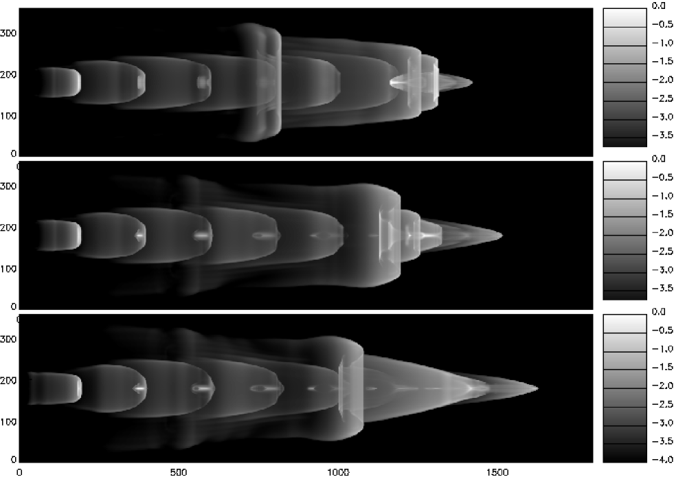
Figure 3: H$\alpha$ emission maps for the three computed models. The frames correspond to the HD, weak MHD ($\beta=1$), and strong MHD ($\beta=0.4$) models (up to bottom), after 500 yrs integration time. The right bar gives the logarithm of the H$\alpha$ emission, normalized to the maximum value of each frame. The axes are labeles in pixels, and the displayed domain has a physical size of ($L_{z}$,$L_{r}$) = ($3\times 10^{17}$, $3\times 10^{16}$) cm. A pixel correspond to a physical size of $1.66\times 10^{14}$ cm.

We choose a toroidal field geometry for two reasons. The first one is that a toroidal magnetic field is necessary to collimate the jet during the ejection-collimation process, and would then also have to be present in the propagating jet. The second reason is that in shocks, the “important” component of the magnetic field is the one parallel to the surface of the shock (which is the toroidal component in our geometry). In fact, all of the previous simulations confirm this idea. Stone & Hardee (SH2000 (2000)) and Frank et al. (Fal1998 (1998)) obtained relevant differences in MHD jets (with respect to the HD case) with a strong toroidal component of the magnetic field, and less important differences for a longitudinal magnetic field (see also Gardiner et al. Gal2000 (2000)). Cerqueira & de Gouveia Dal Pino (2001a , 2001b ) also showed that larger effects in the calculated H$\alpha$ emission are also obtained for toroidal field configurations.

We have computed models with different magnetic field intensities, ranging from $B_{m}=0$ to $B_{m}=93.2$ $\mu$G (see equation 9), corresponding to $\beta=\infty$ to $\beta=0.4$, (where $\beta=2P_{gas}/B^{2}$). In all of our simulations, the ambient medium is not magnetized. The sound velocity and the Alfvén velocities, at the centre of the initial cross section, ranges from c${}_{s,0}=$c${}_{s,amb}/\sqrt{5}\approx 4.5$ km/s and c${}_{A}=0$ (for the $\beta=\infty$ case) to c${}_{s,0}\approx 10$ km/s and c${}_{A}\approx$ 17.3 km/s (for the $\beta=0.4$ case).

3 Results

3.1 General Results

The stratification of the numerical density for simulations with different values of the magnetic field intensity are shown in Fig. 1 for a $t=500$ yr time integration. The top frame shows the HD simulation, the central frame a weak magnetic field simulation (with $\beta$=1, $B_{m}=58.9\,\mu$G) and the bottom frame a strong magnetic field simulation ($\beta$=0.4, $B_{m}=93.2\,\mu$G).

The results show an increasing collimation for increasing toroidal magnetic fields. The knots are due to the imposed variable injection velocity (see Eq. 8). The head of the jet presents a very complicated structure, due to the presence of instabilities (see, e. g., Blondin et al. 1990) and to the interaction of successive knots which catch up with the head.

An important result is that the H$\alpha$ emission of the leading head is strongly dependent on $\beta$. This is a result of the fact that our magnetized jet simulations develop ”nose cones”. These structures are of somewhat dubious reality, as they might disappear in 3D jets without perfect axisymmetry (see Cerqueira & de Gouveia Dal Pino 2001b ).

The structure of the head is strongly time-dependent, and will not be considered in the following analysis. In Fig. 2 we show the density, the ionization fraction, the axial flow velocity and the temperature as a function of position along the symmetry axis for the three computed models. This figure does not include the region of the head of the jet.

Some effects due to the presence of the magnetic field are evident. We see that the on-axis ($r=0$) density increases $\sim$ one order of magnitude from the HD to the $\beta$=0.4 model. The initial temperature is bigger for the magnetized cases due to the different pressure profiles present in the initial configuration of the jet (which correspond to temperature profiles, as the density is assumed to be constant, see section 2) . However, within the internal working surfaces we obtain lower temperatures as a function of increasing magnetic field intensity (similar results were obtained by Stone & Hardee SH2000 (2000)). The ionization fraction in the central regions of the knots decreases as a function of increasing magnetic field strength (which is consistent with the temperature decrease described above).

The separation between the two shocks of the knots increases both as a function of distance from the source and of increasing magnetic field intensity. This latter effect is due to the fact that the magnetic field tends to stop the lateral expansion of the material within the knots, so that more material remains in the region close to the symmetry axis. With respect to the velocity, we see that the shock velocities (which correspond to the velocity jumps observed at the edges of the knots in Fig. 2) increase as a function of increasing magnetic field. Finally, the propagation velocity of the head of the jet increases substantially as a function of increasing magnetic field (as can be seen in Fig. 1). This effect is also due to the increased collimation obtained for the MHD jets.

3.2 Intensity maps

From our models, we have computed H$\alpha$ emission line maps from the models. These maps are obtained integrating the emission coefficient along lines of sight, and are computed assuming an optically thin jet moving parallel to the plane of the sky. In Fig. 3 we show the H$\alpha$ emission line maps predicted from the models presented in Fig. 1. It is evident that the H$\alpha$ emission is more concentrated to the jet axis in the magnetic jet models than in the HD jet.

To have a quantitative value of the H$\alpha$ emission from the knots, we integrate the emission over regions around each knot. To this effect, we integrate the emission within circular diaphragms with a radius of $7\times 10^{15}$ cm centered on the successive knots. In fact, the regions outside these diaphragms have negligible emission (see Fig. 3).

In Fig. 4, we show the results obtained for the different models. The points represent the ratio of the H$\alpha$ luminosities of the successive knots with respect to the H$\alpha$ lumninosity of the corresponding knot in the HD simulation. For the first knot (located at $z\approx 4R_{J}$) we find that all of the magnetized jet models have almost the same H$\alpha$ luminosity as the HD jet model (i. e., $L_{H\alpha}(MHD)/L_{H\alpha}(HD)\approx 1$). The value of $L_{H\alpha}(MHD)/L_{H\alpha}(HD)$ increases as a function of $z$ in the second and third knots (located at $z\approx 8$ and 14$R_{J}$) and then decreases again for larger $z$ values (i. e., for the fourth and fifth knots, located at $z\approx 19$ and $25R_{J}$).

From this Fig. 4, we also see that a model with $\beta=5$ ($B=26.3\mu$G) produces knots with H$\alpha$ luminosities which are basically indistinguishable from the HD simulation. For higher magnetic fields (i. e., for lower values of $\beta$), knots with increasingly larger H$\alpha$ luminosities (compared to the HD case) are obtained. The largest increase is found for the knot at position $z\approx 14r_{j}$ ($\approx 8.5\times 10^{16}$ cm) These results agree at least qualitatively with the ones shown in Fig. 3 of Cerqueira and de Gouveia Dal Pino (2001a ), who find increases in the H$\alpha$ luminosity by factors of $\sim 3$-4 with respect to the HD case for a $\beta=1$ magnetized jet model.

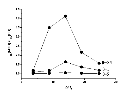
Figure 4: Ratios of the H$\alpha$ luminosities of the knots along magnetized jet models with respect to the H$\alpha$ luminosity of the corresponding knots in a HD jet, as a function of knot position along the jet axis. These luminosities have been obtained by integrating the H$\alpha$ intensity over circular diaphragms centered on the successive knots (see the text and Fig. 3).

4 Conclusions

We have presented 2D numerical simulations of HD and magnetized, variable jets propagating in a homogeneous medium. Models with increasing magnetic fields show an increase in the H$\alpha$ luminosities of the successive knots (which correspond to internal working surfaces which result from the injection velocity variability). This result confirms the work of Cerqueira & de Gouveia Dal Pino (2001a , 2001b ), who estimated the H$\alpha$ luminosity of the clumps along MHD jet simulations using a fit to predictions of plane-parallel shock models.

Somewhat surprisingly, our work presents the first predictions of emission line maps from MHD HH jet models. Therefore, our calculations for the first time show the emission line morphologies that would be expected for such models.

We find that the H$\alpha$ emission of the leading head of the jet differs quite strongly between the HD and MHD cases. This is a result of the fact that our simulations develop extended “nose cones” (of somewhat dubious reality, as these structures might disappear in 3D jets without perfect axisymmetry, see Cerqueira & de Gouveia Dal Pino 2001b ).

For the knots along the jet, we find that for increasing magnetic field strengths we obtain emission structures with stronger peaks towards the symmetry axis. This can be clearly seen in Fig. 3, in which the $\beta=0.4$ model has knots which are dominated by an elongated emission component along the jet axis.

This different type of knot morphology is interesting in terms of observations of HH jets. It has been a long-standing fact that while some HH jets (notably HH 111, see e. g. Reipurth et al. Ral1997 (1996)) show compact knots with “bow shock-like” morphologies which resemble the predictions from HD variable jet models (see Masciadri et al. Mal2002 (2002)), other HH jets (e. g., HH 30, see Lopez et al. Lal1995 (1995)) have emission knots with axially elongated structures. This second kind of morphology could not be modeled successfully in terms of variable HD jet models, and suggested the presence of a different mechanism for knot formation. We now find that variable jets with a strong enough toroidal magnetic field do lead to the formation of axially elongated knots, which in principle might be used to model objects such as HH 30.

The present paper is limited to a study of the effect of a toroidal magnetic field on the H$\alpha$ emission of variable jet flows. In a future paper, we will present a study of a more extended set of emission lines. From such a study, we will attempt to produce a set of line diagnostics which could be used to estimate the magnetic field strength along observed HH jets.

- (1) Aller, L. H. 1984, Physics of Thermal Gaseous Nebulae, Astrophysics & Space Science Library vol. 112
- (2) Biro, S. , Raga, A. C. & Cantó, J., 1995, MNRAS, 275, 557
- (3) Blandford, R. D. & Payne, D. G., 1982, MNRAS, 199, 883
- (4) Blondin, J. M., Fryxell, B. A., & Konigl, A., 1990, ApJ,360,370
- (5) Cerqueira, A. H. & de Gouveia Dal Pino, E. M., 2001a, ApJ, 550, L91
- (6) Cerqueira, A. H. & de Gouveia Dal Pino, E. M., 2001b, ApJ, 560, 779
- (7) Cerqueira, A. H. & de Gouveia Dal Pino, E. M., 1999, ApJ, 510, 828
- (8) Cerqueira, A. H., de Gouveia Dal Pino, E. M. & Herant, M., 1997, ApJ, 489, L185
- (9) Cox, D., PhD Thesis, Univ. California (USA)
- (10) Dalgarno, A. & McCray, R. A, 1972, ARA&A, 10, 375
- (11) De Colle, F., 2005, PhD Thesis, UNAM (México)
- (12) De Colle, F. & Raga, A. C, 2004, AP&SS, 293, 173
- (13) Falle, S. A. E. G., 1991, MNRAS, 250, 581
- (14) Falle, S. A. E. G., Komissarov, S. S., & Joarder, P., 1998, MNRAS, 297, 265
- (15) Frank, A., Gardiner, T. A., Delemarter, G. & Lery, T., 1999, ApJ, 524, 947
- (16) Frank, A., Ryu, D., Jones, T. W., & Noriega-Crespo, A., 1998, ApJ, 494, L79
- (17) Gardiner, T. A., Franck, A., Jones, T. W. & Ryu, D., 2000, ApJ, 530, 834
- (18) Giovanardi, C. & Palla, F., 1989, A&AS, 77, 157
- (19) Hartigan, P., Morse, J. A., & Raymond, J., 1994, ApJ, 436, 125
- (20) Lind, H., Payne, D., Meier, D. & Blandford., R., 1989, ApJ, 344, 89
- (21) Lopez, R., Raga, A., Riera, A., Anglada, G. & Estalella, R., 1995, MNRAS, 274, L19
- (22) Masciadri, E., Velázquez, P. F., Raga, A. C. & Noriega-Crespo, A., 2002, ApJ, 573, 260
- (23) Raga, A. C., 1994, Ap&SS, 216, 105
- (24) Raga, A. C., Binette, L., Cantó, J. & Calvet, N., 1990, ApJ, 364, 601
- (25) Reipurth, B., 1989, Nature, 340, 42
- (26) Reipurth, B. & Bally, J., 2001, ARA&A, 39, 403
- (27) Reipurth, B., Hartigan, P., Heathcote, S., Morse, J. A. & Bally, J., 1997, AJ, 114, 757
- (28) O’Sullivan S. & Ray, T. P., 2000, A&A, 363, 355
- (29) Ryu, D., Jones, T. W. & Frank, A., 1995, ApJ, 452, 785
- (30) Stone, J. M., & Hardee, P. E., 2000, ApJ, 540, 192
- (31) Schwartz, R. D., 1975, ApJ, 195, 631
- (32) Todo, Y., Uchida, Y., Sato, T. & Rosner, R., 1993, ApJ, 403, 164
- (33) Toth, G., 2000, JCP, 161, 605
- (34) Uchida, Y. & Shibata, K., 1985, PASJ, 37, 515
- (35)