Kinemetry: a generalisation of photometry to the higher moments of the line-of-sight velocity distribution

Abstract

We present a generalisation of surface photometry to the higher-order moments of the line-of-sight velocity distribution of galaxies observed with integral-field spectrographs. The generalisation follows the approach of surface photometry by determining the best fitting ellipses along which the profiles of the moments can be extracted and analysed by means of harmonic expansion. The assumption for the odd moments (e.g. mean velocity) is that the profile along an ellipse satisfies a simple cosine law. The assumption for the even moments (e.g velocity dispersion) is that the profile is constant, as it is used in surface photometry. We test the method on a number of model maps and discuss the meaning of the resulting harmonic terms. We apply the method to the kinematic moments of an axisymmetric model elliptical galaxy and probe the influence of noise on the harmonic terms. We also apply the method to SAURON observations of NGC 2549, NGC 2974, NGC 4459 and NGC 4473 where we detect multiple co- and counter-rotating (NGC 2549 and NGC 4473 respectively) components. We find that velocity profiles extracted along ellipses of early-type galaxies are well represented by the simple cosine law (with 2% accuracy), while possible deviations are carried in the fifth harmonic term which is sensitive to the existence of multiple kinematic components, and has some analogy to the shape parameter of photometry. We compare the properties of the kinematic and photometric ellipses and find that they are often very similar, but a study on a larger sample is necessary. Finally, we offer a characterisation of the main velocity structures based only on the kinemetric parameters which can be used to quantify the features in velocity maps.

1 Introduction

Over the last three decades broad band observations of early-type galaxies were successfully analysed by a method commonly called surface photometry or, simply, photometry. This method is based on the analysis of isophotal shapes of the projected surface brightness. The development of the method was stimulated by the empirical discovery that the isophotes of early-type galaxies are reproduced by ellipses to better than 1 per cent (Kent, 1984; Lauer, 1985b; Davis et al., 1985; Jedrzejewski, 1987; Peletier et al., 1990). Although the isophotes are elliptical in shape to high accuracy, under careful examination, many isophotes of early-type galaxies do show differences from pure ellipses at a level of $\approx 0.5\%$ (e.g. Bender et al., 1988; Peletier et al., 1990). The true success of photometry was the ability to measure these deviations and classify early-type galaxies accordingly into disky and boxy objects (Lauer, 1985a; Jedrzejewski, 1987; Bender & Moellenhoff, 1987). When combined with information on total luminosity and spatially resolved spectroscopy, it followed that the duality of photometric properties of early-type galaxies is reflected in a duality of kinematic properties, where faint disky objects were found to rotate faster than luminous boxy objects (Davies et al., 1983; Davies & Illingworth, 1983; Bender, 1988; Nieto et al., 1988; Wagner et al., 1988; Bender et al., 1989; Nieto & Bender, 1989; Busarello et al., 1992; Bender et al., 1994). High resolution imaging studies with the Hubble Space Telescope (Jaffe et al., 1994; Lauer et al., 1995; Rest et al., 2001), again based on photometric analysis, revealed new properties of early-type galaxies that deepened the division of the galaxies in two groups. These remarkable set of discoveries resulted in a revised classification scheme of galaxies (Kormendy & Bender, 1996).

It is fair to say that our increased knowledge of early-type galaxies (partially) comes from photometry and the ability of the method to harvest and describe in a compact way the information from two-dimensional images. However, the integrated light remains a limited source of information about the internal structure and thus the true nature of galaxies. Kinematic information is also essential to fathom the complexity of galaxies and, especially, two-dimensional kinematic information is required (e.g. Franx et al., 1991; Statler, 1991; Statler & Fry, 1994; Statler, 1994a, b; Arnold et al., 1994).

Two-dimensional velocity maps were, until recently, only possible for objects with clear emission lines. Such maps were the result of studies of, e.g., HI with radio interferometers, (e.g. Swaters et al., 2002), CO with millimetre interferometers (e.g. Helfer et al., 2003) and H$\alpha$ with Fabry-Perot spectrographs (e.g. Hernandez et al., 2005). The advent of integral-field spectrographs (e.g. TIGER, OASIS, SAURON, PMAS, GMOS, SINFONI, OSIRIS), however, has brought two-dimensional kinematic measurements to classical optical and near-infrared wavelengths. Here it is possible to probe both the stellar absorption- and gas emission-lines, which may co-exist in the same potential with very different spatial distributions and dynamical structures. The wealth of features seen in stellar kinematic maps of early-type galaxies (Emsellem et al., 2004) confirms the usefulness of two-dimensional data, but also poses a problem to efficiently harvest and interpret the important features from the maps.

An approach using harmonic expansion was developed for the analysis of two-dimensional velocity maps of disk galaxies. This method divides a velocity map into individual rings (the so-called tilted-ring method, Begeman, 1987) and performs a harmonic expansion along these rings (e.g. Binney, 1978; Teuben, 1991; Franx et al., 1994; Schoenmakers et al., 1997; Wong et al., 2004). This analysis, however, is based on the assumption that the emission-line emitting material is confined to a thin disk structure. Clearly, a spheroidal distribution of stars typical of early-type galaxies does not have the same dynamical properties as a gas disk. To explore those intrinsic properties, one needs a more general method which will not be based on assumptions about the nature of the observed system (e.g. a disk), but will rely solely on the properties of the investigated observables (e.g. surface brightness or velocity).

Here we explore such a general method. Photometry earned its spurs in intensive applications over the last three decades and offers a natural starting point for the analysis of two-dimensional kinematic maps, although one can, in principle, invent a number of basis functions which can describe a two-dimensional distribution. In this paper, we present a generalisation of photometry to the higher-order moments of the line-of-sight velocity distribution (LOSVD). This generalisation is based on the theoretical fact that surface brightness is itself a moment of the LOSVD, and on our empirical discovery that the velocity maps of many early-type galaxies can be well reproduced by a simple cosine law along sampling ellipses. We call our method kinemetry, which reduces to photometry for the investigation of surface brightness distributions.

In Section 2 we present the theoretical background and motivation for the new method. Section 3 presents the technical aspects of the method. The meaning of the kinemetric coefficients and their diagnostic merits for different model maps are presented in Section 4. In Section 5 we apply the method on kinematic maps of an axisymmetric model galaxy, present the application of kinemetry to actual observations and characterise typical structures on velocity maps. We summarise our conclusions in Section 6.

2 Theoretical background and motivation

The dynamics of a collisionless stellar system is fully specified by its phase-space density or distribution function $f=f(\vec{x},\vec{v},t)$ (e.g. Binney & Tremaine, 1987), but this quantity is not measurable directly. When observing external galaxies, we measure properties that are integrated along the line-of-sight (LOS). An additional complication is that the galaxies are viewed from a certain direction, and we actually observe only those projected properties of the integrated distribution function.

The observables, which reveal only averages over a large number of unresolved stars, are the surface brightness and the LOSVD, sometimes also called the velocity profile (for a review see de Zeeuw, 1994). The surface brightness is given by

$$\mu(x,y)=\int_{\mathrm{LOS}}\mathrm{d}z\int\!\int\!\int\!\mathrm{d}\vec{v}\,f(\vec{r},\vec{v}).$$ (1)

The rest of the observable information is carried by the LOSVD, which relates to the distribution function via

$$\mathcal{L}(v;x,y)=\int_{\mathrm{LOS}}\mathrm{d}z\int\!\int\!\mathrm{d}v_{x}\mathrm{d}v_{y}\,f(\vec{r},\vec{v}),$$ (2)

where (x,y,z) are the three spatial coordinates, oriented such that the LOS is along the z-axis. From these equations it is trivial to show that surface brightness is the zero-th order moment of the LOSVD. Higher-order moments, such as $\langle V\rangle$, or $\langle V^{2}\rangle$, can easily be related to the observables of the LOSVD: mean velocity $V$, velocity dispersion $\sigma$ and higher-order moments, commonly parametrised by Gauss-Hermite coefficients (van der Marel & Franx, 1993; Gerhard, 1993), $h_{3}$ and $h_{4}$ being the most used.

The kinematic moments of stationary triaxial systems show a high degree of symmetry which can be expressed through their parity. The mean velocity is an odd moment, while the velocity dispersion is an even moment. In practice, this means that a two-dimensional map of a given moment shows corresponding symmetry. Maps of even moments are point-symmetric, while maps of odd moments are point-anti-symmetric. In polar coordinates on the sky plane this gives:

$$\mu_{e}(r,\theta+\pi) = \mu_{e}(r,\theta),$$

$$\mu_{o}(r,\theta+\pi) = -\mu_{o}(r,\theta),$$ (3)

where $\mu_{e}$ and $\mu_{o}$ are arbitrary even and odd moments of the LOSVD, respectively. Furthermore, if the observed system is axisymmetric, the even moment of the LOSVD will also be mirror-symmetric or, correspondingly, an odd moment will be mirror-anti-symmetric:

$$\mu_{e}(r,\pi-\theta) = \mu_{e}(r,\theta),$$

$$\mu_{o}(r,\pi-\theta) = -\mu_{o}(r,\theta).$$ (4)

A kinematic moment that satisfy both symmetries (eqs. 2 and 2) is said to be bi-(anti)-symmetric. The existence of these symmetries can be used to simplify the harmonic analysis. Point-symmetric moments give rise only to even harmonic terms, while point-anti-symmetric moments will require only odd harmonic terms. Mirror-(anti)-symmetry additionally requires that there is no change in the moment’s position angle. For a more detailed discussion on the influence of these equations on the terms of the harmonic expansion see Appendix A.

Following these conventions, surface brightness, as the zeroth order moment, is an even moment. As the surface brightness and the kinematic moments of the LOSVD are moments of the same distribution function, it is natural to analyse them similarly, and we can ask in which way one can generalise the method of photometry to work on the higher moments of the LOSVD. Considering symmetry, the even moments do not require much change in the method, but the odd moments need a new working assumption. Also, while the isophotes of integrated light are elliptical to a high accuracy, the choice of sampling curves is not as obvious for odd kinematic moments.

Since the light distribution of early-type galaxies is elliptical it is reasonable to assume that an expansion along ellipses would also be suitable for the extraction of profiles from kinematic moment maps giving some insight in their structure and properties. The choice of the actual ellipticity, however, is somewhat arbitrary. For example, it is possible to expand along the galaxy isophotes or along ellipses that correspond to deprojected circles. In the first case, one follows the photometry and probes regions of the same projected surface brightness. In the second case, one samples locations with equal intrinsic radii, but it is necessary to assume an inclination for the galaxy, which is usually difficult to estimate. It may also not be physically justified to use a constant ellipticity for the whole velocity map, as the ellipticity of the light distribution may change with radius.

As a special case, it is possible to expand a kinematic map along circles. This approach was investigated by Copin et al. (2001), Copin (2002) and Krajnović (2004), and although it is straight-forward and requires no a priori assumption, a large number of harmonic terms are often necessary, preventing a simple description of the maps and complicating the analysis (see Appendix A for a discussion). Additionally, an expansion along ellipses can reduce to expansion along circles in limiting cases (see section 4.3). Franx et al. (1989) also note the advantages of extraction along circles, even for photometry, but conclude that an approach based on ellipses is superior.

Consider the first moment of the LOSVD, the mean velocity. In specific cases, the geometry of the system offers a choice for curves along which velocity profiles can be extracted. If a velocity map traces material in a thin disk, such as is often the case in HI, CO and H$\alpha$ gas emission maps, velocity can be well represented by circular motion. If the inclination of the disk is known, a circular orbit in the plane of the galaxy can be projected as an ellipse on the sky. A velocity profile extracted along this ellipse is then of simple cosine form, which can be expressed by

$$V(R,\psi)=V_{0}+V_{C}(R)\sin i\cos\psi,$$ (5)

where $R$ is the radius of a circular ring in the plane of the galaxy (or the semi-major axis length of the ellipse on the sky), $V_{0}$ is the systemic velocity, $V_{C}$ is the ring circular velocity, $i$ is the ring inclination ($i=0$ for a ring seen face-on) and $\psi$ is the azimuthal angle measured from the projected major axis in the plane of the galaxy. The inclination $i$ is related to the axial ratio or flattening, $q$, of the ring’s major and minor axes. For a given flattening, the ring’s velocity profile is most similar to the velocity of a circular orbit with radius $R$ and inclination $\cos i=q$. In other words, the flattening defines an ellipse on the sky, with ellipticity $\epsilon=1-q$, which corresponds to a circle describing the orbits in the plane of the galaxy.

If one assumes that the velocity profiles extracted from velocity maps (either stellar or gaseous) of early-type galaxies can be described by the simple cosine law of eq. (5) to a high accuracy, then the first step in the analysis of velocity maps is to determine those ellipses along which the velocity profile is best described by eq. (5). In analogy with photometry, the next step would be to determine the deviations of the velocity profile from the cosine law, which can be achieved by the higher-order Fourier analysis.

We discovered that the velocity profiles extracted from the maps of the SAURON sample can indeed be well described by the cosine law of eq. (5). Note that this observation suggests that the velocity maps of early type galaxies closely resemble the observed kinematics of inclined circular disks. One has, however, to take a step back and recognise that spheroids are not disks, and the two cases should be clearly differentiated during the interpretation of the results. The fact that the velocity maps of galaxies are well approximated by the thin disk model allows us to develop a simple generalisation of photometry based on eq. (5), but also reflects an interesting property of the internal structure of galaxies, which is worth exploring further (see section 5.2 for a few examples while the results for the rest of the SAURON sample will be reported in a future paper).

The method presented in this paper is applicable to all moments of the LOSVD. The quality of kinematic data, however, usually decreases rapidly with increasing order of the kinematic moment: the signal is generally simply too weak for a good enough extraction of the higher-order moments from raw data. Perhaps it is even fair to say that only the mean velocity maps reach the quality of photometric observations from thirty or so years ago, when surface photometry was introduced. For these reasons, as well as for presentation purposes, we restrict our analysis to the mean velocity maps. The method, however, can be straight-forwardly applied to the higher order moments (see Section 5.1 for an example).

3 The method

In this section we present the details of the new algorithm extending surface photometry to the maps of odd moments of the LOSVD.

3.1 Harmonic expansion

Fourier analysis is the most straight-forward approach to characterise any periodic phenomenon. A velocity map $K(a,\psi)$ can be divided into a number of elliptical rings yielding velocity profiles which can be described by a finite (and small) number ($N+1$) of harmonic terms (frequencies):

$$K(a,\psi)=A_{0}(a)+\sum_{n=1}^{N}A_{n}(a)\,\sin(n\psi)+B_{n}(a)\,\cos(n\psi),$$ (6)

where $\psi$ is the eccentric anomaly, that in case of disks corresponds to the azimuthal angle of eq. (5), and $a$ is the length of the semi-major axis of the elliptical ring.

As presented by Carter (1978), Kent (1983) and Jedrzejewski (1987), to find the best sampling ellipse along which a profile $\mu_{e}$ should be extracted, one minimises the harmonic terms sensitive to the parameters of the ellipse (centre, position angle and ellipticity for a given semi-major axis length). In the case of an even moment (e.g. surface brightness) the best fitting ellipse parameters are given by minimising $A_{1}$, $B_{1}$, $A_{2}$ and $B_{2}$ coefficients of the harmonic expansion. This means that a photometric ellipse is determined when a sufficiently good fit to $\mu_{e}(a,\psi)=A_{0}(a)$ is obtained. In the case of an odd moment of the LOSVD (e.g. mean velocity), given our empirical finding, the sampling ellipse parameters are determined by requiring that the profile along the ellipse is well described by eq. (5), or, generally, $\mu_{o}(a,\psi)=B_{1}(a)\cos\psi$.

Ellipse parameters (position angle, centre and flattening) can be determined by a minimising a small number of harmonic terms. In Appendix B we investigate which terms are sensitive to changes of the ellipse parameters. We find that:

• an incorrect kinematic centre produces non-zero $A_{0}$, $A_{2}$, $B_{2}$, and to a lower level $A_{1}$, $A_{3}$ and $B_{3}$ coefficients,

• an incorrect flattening (inclination) produces a non-zero $B_{3}$ coefficient,

• an incorrect position angle produces non-zero $A_{1}$, $A_{3}$ and $B_{3}$ coefficients.

In the study of disk velocity maps, Schoenmakers et al. (1997) in their Appendix A2, discuss the same sensitivity, but for small deviations. In this limit, our results reduce to the analytically derived conclusions of Schoenmakers et al. (1997). It is, however, important to note, that whatever the combination of incorrect centre, flattening or position angle, only the $n\leq 3$ harmonic terms are affected.

3.2 The algorithm

Given our discovery that the cosine law along sampling ellipses describes well velocity maps of galaxies, a small number of harmonic terms is needed to determine the best fitting ellipse. In this case eq. (6) reduces to

$$K(\psi)=A_{0}+A_{1}\,\sin(\psi)+B_{1}\,\cos(\psi)$$

$$+A_{2}\,\sin(2\psi)+B_{2}\,\cos(2\psi)$$

$$+A_{3}\,\sin(3\psi)+B_{3}\,\cos(3\psi)$$ (7)

where $\psi$ is the eccentric anomaly. In practice, as it is done in photometry, we sample the points uniformly in $\psi$ and the ellipse coordinates are then given by $x_{e}=a\cos\psi$ and $y_{e}=q\,a\sin\psi$. This implies that, if the ellipse is projected onto a circle, the sampling points are equidistant. The selection of $K(\psi)$ values is obtained by a bilinear interpolation of the observed map, also in the same way it is usually done in photometry (Jedrzejewski, 1987).

The parameters of the best sampling ellipse for an odd kinematic moment are obtained by minimising:

$$\chi^{2}=A^{2}_{1}+A^{2}_{2}+B^{2}_{2}+A^{2}_{3}+B^{2}_{3}$$ (8)

from eq. (3.2). This non-linear fit is performed in two stages. The first stage consists of minimising $\chi^{2}$ on an input grid of flattenings $q$ and position angles $\Gamma$. The second stage repeats the fit using a non-linear least-square curve fitting algorithm, but now also fitting for the coordinates of the centre, taking as initial values $q=q_{min}$ and $\Gamma=\Gamma_{min}$ from the first stage and an estimate of the centre ($x_{0},y_{0}$). In this way, the true $\chi^{2}$ minimum can be robustly determined and, hence, the parameters of the best sampling ellipse: centre ($x_{c},y_{c}$), flattening (ellipticity) and position angle. We use the MINPACK implementation (Moré et al., 1980) of the Levenberg-Marquardt method. This two stage approach was implemented to improve the robustness of the method, preventing the minimisation program from choosing possible secondary minima.

The choice for the length of semi-major axis of consecutive ellipses is set by the decrease of surface brightness of the observed object. The kinematic maps are necessarily spatially binned (e.g. using adaptive Voronoi binning (Cappellari & Copin, 2003), as in the examples of Section 5), and as the bins typically increase in size with radius, the distance between the rings has to be increased to avoid correlation between the ring parameters. The correlation should also be avoided in the centre where the bins are usually identical to the original pixels. For these reasons, we adopted a combination of linear and logarithmic increase of the semi-major axis length given by this expression: $a=n+1.1^{n}$, where $n=1,2,3...$.

The final ellipse parameters obtained by minimisation are then used to describe an elliptical ring from which a kinematic profile is extracted and expanded onto the harmonic series of eq. (6), where the coefficients $(A_{n},B_{n})$ are determined by a least-squares fit with a basis $\{1,\cos\psi,\sin\psi,...,\cos N\psi,\sin N\psi\}$.

The harmonic series can be presented in a more compact way,

$$K(a,\psi)=A_{0}(a)+\sum_{n=1}^{N}k_{n}(a)\,\cos[n(\psi-\phi_{n}(a))].$$ (9)

where the amplitude and phase coefficients ($k_{n}$, $\phi_{n}$) are easily calculated from the $A_{n},B_{n}$ coefficients:

$$k_{n}=\sqrt{A^{2}_{n}+B^{2}_{n}}\phantom{10}\textrm{and}\phantom{10}\phi_{n}=\arctan\left(\frac{A_{n}}{B_{n}}\right).$$ (10)

The $\sin$ and $\cos$ terms have different properties and, in principle, describe different characteristics of the maps. The properties of the corresponding coefficients have been studied and described for the case of thin gaseous disks (Franx et al., 1994; Schoenmakers et al., 1997; Wong et al., 2004). In a general case however, namely for the analysis of kinematic maps of triaxial (stellar) systems, those properties do not apply (e.g. the $b_{1}$ term represents circular rotation only in the thin disk approximation). For these reasons, we find it more instructive in this paper to combine the coefficients of the same order and characterise the global properties of kinematic maps. In what follows, although the implementation of the method determines individual coefficients (and can be straight-forwardly used for the special cases of disks), they will be presented in the spirit of eq. (9).

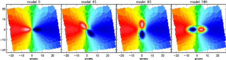
Figure 1: Four model maps representing different but typical velocity maps of triaxial early-type galaxies. Velocity maps were constructed of two components (see text for details). The position angle of the first (nuclear) component changes from left to right: 0, 45, 90 and 180°. The size of bins increases towards the edge of the maps, as expected form observations, to keep constant signal-to-noise ratio. Note also the different opening angles of the two components on the maps.

3.3 Internal error estimates

The uncertainties of the resulting parameters can be estimated from the measurement errors of the input kinematic data. The ellipse parameters determined by the Levenberg-Marquardt least-squares minimisation code have formal one-sigma uncertainties computed from the covariance matrix. If an input parameter is held fixed, or if it touches a boundary, then the error is reported as zero. Similarly, the harmonic terms obtained in the linear least-squares fit in the second part of the procedure have their formal one-sigma errors estimated from the diagonal elements of the corresponding covariance matrix, as described in Section 15.6 of Press et al. (1992).

We performed Monte Carlo simulations to estimate the robustness of the obtained internal errors. We used the SAURON (Bacon et al., 2001) velocity map of NGC 2974 presented in Emsellem et al. (2004) and its measurement errors to construct one hundred realisations of the velocity map. The velocity in each bin was taken from a Gaussian distribution of mean equal to the observed velocity and standard deviation given by the corresponding measurement error. Typical errors on the velocities of the SAURON observations are about $5\>{\rm km}\,{\rm s}^{-1}$. All realisations provide a distribution of values from which we estimate one-sigma errors. The Monte Carlo uncertainties are in a good agreement with the formal errors. Note, however, that these errors are statistical errors only and do not include systematic effects. We investigate the resulting accuracy of the kinemetric coefficients in Section 5.

4 Kinematic parameters and their meaning

The crucial aspect of any analysis method is the interpretation of its results. In this section, we describe in more detail the way the method works and demonstrate the meaning of the resulting kinemetric parameters.

4.1 Model velocity maps

We constructed a set of model velocity maps combining two components using the circular velocity from the Hernquist (1990) potential, weighted with two different surface brightness distributions. The Hernquist potential was chosen because it approximates reasonably well the density of real early-type galaxies. Its circular velocity is given by $V_{c}=\sqrt{GMr}/(r+r_{0})$, where $G$ is the gravitational constant, $M$ is total mass of the system, and $r_{0}$ is scale length of the potential. The $\sqrt{GM}$ factors for the two components were 850 and 1500 (in units of $\>{\rm km}\,{\rm s}^{-1}$ arcsec^1/2), respectively, while $r_{0}$ scale lengths were set to 5″and 15″, defining a central and large scale component, respectively.

The light distribution of the first component was described by an exponential law typical of disks, and that of the second component by an $r^{1/4}$ law typical of spheroids. They were both normalised to a maximum value of unity. The light distribution scale lengths, $r_{e}$, of the two components were set to 7″and 15″, respectively. The components were inclined (60°and 40°, respectively) and combined with 4:1 relative weights, respectively, rotating the central component for different position angles $\Gamma=(0\degr,45\degr,90\degr,180\degr)$ in order to construct different features on velocity maps possible to occur in triaxial early-type galaxies.

The final result are four model velocity maps, which satisfy the symmetry relations of eq. (2), presented in Fig. 1. Each model has a distinct nuclear component with a somewhat higher maximum velocity and a smaller opening angle than the large scale, spheroidal component. We define the opening angle loosely as a quantity that describes the tightness of the iso-velocity contours. It is discussed in more detail below. The main difference between the models is in the orientation of the nuclear component. All model maps were constructed to simulate realistic observations with the SAURON integral-field spectrograph, where the size of the spatial bins increases from the centre outwards to maintain constant signal-to-noise ratio.

Figure 2: Kinemetric coefficients of the model maps. From left to right the plots show the results for model 0, model 45, model 90 and model 180. From top to bottom: kinematic position angle $\Gamma$, flattening $q$, coefficients of harmonic expansion $k_{1}$ and $k_{5}/k_{1}$. Note that the sudden rise of $k_{5}/k_{1}$ in model 180 at 9″is due to the nearly zero value of the rotation velocity $k_{1}$ at that radius.

4.2 Kinemetric analysis of model maps

The parity of an odd kinematic moment guarantees that the even terms in the expansion vanish in the absence of measurement errors and assuming that the centre is given correctly. These conditions are satisfied for the model velocity maps and, while applying the algorithm of section 3.2, we simplified eqs. (3.2) and  (8) by not minimising the contribution of $A_{2}$ and $B_{2}$. However, during the harmonic analysis we expanded the extracted velocity profiles including two additional odd harmonic terms, $A_{5}$ and $B_{5}$, which describe the deviations from circular rotation (see eq. 5).

A special case is that of the zeroth-order term given by the $A_{0}$ coefficient. It is not shown in the subsequent analysis because the absolute level of the maps was set to zero by construction. For velocity maps, $A_{0}$ gives the systemic velocity of each ring. In the case of even kinematic moments, the meaning of $A_{0}$ is different: it is the dominant term describing the amplitude of the moment (e.g. intensity for surface brightness, amplitude for velocity dispersion of velocity dispersion maps, see section 5.1).

Figure 2 shows the kinemetric parameters which describe the model velocity maps. All parameters are plotted versus the semi-major axis length of the ellipses. The first and second row show the orientation ($\Gamma$) and flattening ($q$) of the ellipse along which the velocity profile was extracted. These parameters uniquely specify the best fitting ellipse, along which the contribution of $A_{1}$, $A_{3}$ and $B_{3}$ terms is minimal. The following rows show plots of the harmonic coefficients given in the compact form of eq. (10): $k_{1}$ and $k_{5}/k_{1}$.

The meaning of these parameters can be associated with the visible structures on the maps as follows:

1. $\Gamma$ is the kinematic position angle. Like the photometric position angle, it describes the orientation of the velocity map, and it is related to the projection of the angular momentum vector (see Appendix C). $\Gamma$ traces the position of the maximum velocity on the map.

2. $q$ is the axial ratio or flattening of the ellipse and it describes the flattening of the map. It can be interpreted as a measure of the opening angle of the iso-velocity contours. Maps that have large opening angles appear round (large values of $q$), while maps with small opening angle appear flat (small values of $q$). In the special case of a disk, where the motion is confined to a plane (spiral galaxies, gaseous disks, etc), the flattening is directly related to the inclination of the disk, $q=\cos(i)$, where the projected ellipses correspond to intrinsically circular orbits.

3. $k_{1}$ is the dominant coefficient on maps of odd kinematic moments. For velocity maps, it describes the amplitude of bulk motions (rotation curve). It contains contributions from both $\cos\psi$ and $\sin\psi$ terms, and in the special case of a thin disk geometry, the $A_{1}$ and $B_{1}$ terms should be considered separately. In the case of perfect circular motions ($A_{1}$ and other higher terms are zero), $k_{1}$ describes the full motion on the map. In other words, if higher order coefficients are zero (or negligible), then the velocity map is identical to the velocity map of a disk viewed at inclination $i$.

4. $k_{3}$ is the combination of harmonic coefficients that are minimised in the fitting process. This coefficient is sensitive to the, centre, flattening and position angle of the ellipse and in special cases it will be larger then zero indicating a velocity profile with a complex structure (multiple extremes) originating from the overlap of multiple kinematic components with different orientations (see Fig. 3). This coefficient, however, does not bring any additional information to $q$ and $\Gamma$ and we do not show it. On the other hand, if $q$ and $\Gamma$ are fixed and not fitted, as is often the case in studies of disk velocity maps, then this term brings the first correction to the simple rotational motion.

5. $k_{5}$ is the first higher-order term which does not define the parameters of the best fitting ellipse. It represents the higher-order deviations from simple rotation and points to complex structures on the maps. This term is thus sensitive to the existence of separate kinematic components. It is a kinemetric analogous of the photometric term that describes the deviation of the isophote shape from an ellipse (diskiness and boxiness)

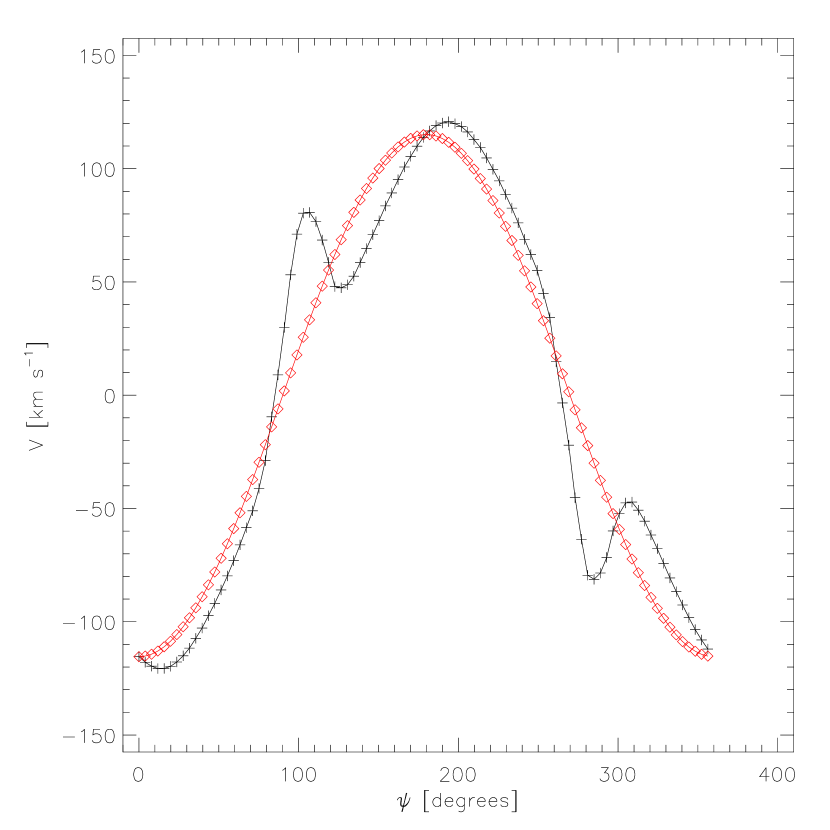
Figure 3: Velocity profile taken from the model 90 map along a circle ($q=1$) at r=9″, in the transition region between the two components. Overplotted with diamonds is the circular velocity profile at the same position. The observed profile exhibits a complex structure which can not be represented by requiring that the third-order terms in the harmonic expansion be zero. The local extremes at $\psi\approx 100\degr$ and $280\degr$ originate in the nuclear component, while the global maximum and minimum are given by the large scale component.

Comparison of the structures on the model maps (Fig. 1) and the radial dependence of the kinemetric coefficients (Fig. 2) illustrates the descriptive power of the method. Our model maps were built of two components which had different flattening and kinematic position angle. It is the role of the kinemetric coefficients to recognise these characteristics and describe them (Fig. 2).

The components of model 0 were aligned, but the nuclear component iso-velocities had a small opening angle, while those of the large-scale component had a large opening angle. This is reflected in the different flattenings $q$. In the inner 10″, the disky component dominates and the map is rather flat, while beyond this region the spheroidal component dominates and the map looks more round. In the regions where only one component dominates, the recovered axial ratio corresponds correctly to the inclination of that component. While the $k_{1}$ terms show the amplitude of the rotation, the $k_{3}$ and $k_{5}$ coefficients are close to zero. This is expected because the models were built of two maps of essentially circular velocity. A small $k_{5}$ terms exists in the transition region between the components. This suggests that the combination of aligned but separate velocity components will give rise to non-zero $k_{5}$.

A confirmation of this effect is given by model 180, where the two components are aligned but counter-rotating. In this configuration the components are clearly visible on the $q$ and $k_{1}$ panels and $k_{5}$ rises strongly in the region coinciding with the change of rotational sense (change in the kinematic position angle by 180°).

Differences in kinematic position angle between the components, as in the maps of model 45 and model 90, generate more power in higher order coefficients. The position angle is recovered correctly in the regions dominated by one component, while in the region between the components it traces the position of (combined) maximum velocity. It is the same with the flattening, which follows the change of the map topology, reaching extreme round values in the transition region where both components equally dominate. The reason for this is the complex shape of the velocity profile, for which it becomes impossible to make the $A_{3}$ and $B_{3}$ terms along any ellipse equal to zero (Fig. 3). In such a case, the fitting routine chooses the equal ratio of axes as this is the most general case, confirming the robustness of the approach. The two stage fit, direct grid fitting followed by non-linear minimisation, is necessary to provide the required robustness in such regions.

The extent of the transition region depends on the relative position angle, larger angles resulting in a larger transition region. This is reflected in the behaviour of the higher-order terms, which become more important and influence a larger area with increasing misalignment of the components. The increasing misalignment is effectively separating the components, creating a complex, multi-peaked velocity profile such as in Fig. 3. Note that strong contribution of higher-order terms in this examples is not necessarily representative of real galaxies, as the features on the velocity maps were not modelled to represent specific observed cases.

Figure 4 shows the two-dimensional representation of the analysis. For each model, we reconstructed a map using only the $b_{1}$ term which is not minimised, and we named those new maps ’circular velocity’. We also reconstructed a map using all 6 terms of the harmonic expansion, which we named ’kinemetric velocity’. The difference between the two velocity maps shows the contribution of the higher order terms ($k_{3}$ and $k_{5}$). These residual maps of model 0 and model 180 show distinct five-fold symmetries coming from the high $k_{5}$ term. Residuals of other models show a combination of the $k_{3}$ and $k_{5}$ terms in the transition region where velocity profiles are similar to the one in Fig. 3

The two examples with five-fold symmetries are interesting when compared with the corresponding model maps. Both residual maps have positive amplitudes on the negative side of the major axis. This is, however, not the case for the model maps. The model 0 map has two components which both rotate in the same direction, while for model 180 the inner component counter-rotates with respect to the outer component. Both models have a strong $k_{5}$ term, and hence five-fold residual structure in the transition region. Interestingly, the amplitude of the residuals of model 180 at e.g. $r=7\arcsec$ along the major axis is negative while the mean rotation at the same radius is positive, belonging to the region dominated by the counter-rotating component. It is thus possible to infer that the residuals actually trace the contribution of the main body rotation in this region, although this is not visible on the velocity map. A similar situation is visible in model 0, but the two components co-rotate and the residuals show the same sense of rotation.

We conclude this exercise stating that $k_{5}$ is sensitive to the existence of different components, where the increase of $k_{5}$ in the presented models is correlated to larger misalignments between the components.

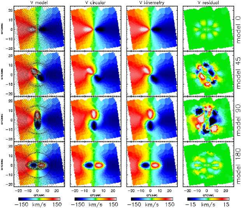
Figure 4: Model velocity maps and the results of the kinemetric analysis. From top to bottom: maps corresponding to model 0, model 45, model 90 and model 180 (as noted at the end of each row). From left to right: model maps, maps of circular velocity, reconstructed model maps using 6 harmonic terms, residual between circular and reconstructed velocity maps. Overplotted on the model maps are the best fitting ellipses along which the velocity profiles were extracted and analysed. Note the change in flattening and position angle of the ellipses.

4.3 Special cases

There are two possible cases of velocity maps for which the determination of kinemetric coefficients will be degenerate. The first case arises from the effect of solid body rotation. As shown in Schoenmakers et al. (1997), while it is possible to measure the position angle $\Gamma(a)$, it is impossible to uniquely determine the flattening $q(a)$, the centre and the systemic velocity. This degeneracy is present because all iso-velocity contours are parallel, and the opening angle is $180\degr$.

Another extreme case occurs when rotation is very slow. Such velocity maps are often found in giant ellipticals which are thought to be triaxial bodies. Here the velocity profiles are roughly constant and do not show the parity expected from an odd moment of the LOSVD. There is no gradient in velocity and as a consequence the flattening and position angle cannot be determined.

In these two cases the new method cannot be applied blindly because it is not possible to interpret harmonic terms in the way we showed up to now. There are two possible ways to proceed. One way is to make an assumption about the flattening and the kinematic position angle (e.g. use photometric flattening), and continue with the harmonic analysis of the velocity profiles extracted along those ellipses.

A more general way, for both cases, is to extract the velocity profiles along concentric circles and perform the harmonic analysis on those. In this way one does not bring any assumption in the analysis, but it is still possible to determine the rotation velocity and kinematic position angle (if present) and detect trends in higher-order harmonic terms. A detailed discussion of extraction along circles and the meaning of the coefficients is given in Appendix A. An automatic transition towards circles can be implemented by adding a penalty term to the $\chi^{2}$, to bias the solution towards round shapes, when the gradient is small (or iso-velocities are parallel). The goodness of fit is then determined by $\chi^{2}_{p}=\chi^{2}+\alpha P(q)$. We also note that an expansion on circles might be good for the analysis of higher-order moments of the LOSVD which normally have rather poor signal-to-noise ratio.

Figure 5: Maps of mean velocity (right), velocity dispersion (middle) $\sigma$, and Gauss-Hermite moment $h_{3}$ (left) for the model galaxy with added intrinsic scatter corresponding to a realistic measurement with SAURON. The overplotted ellipses on the velocity map are the surface brightness contours. The plots in each right and left column represent the kinemetric parameters ($\Gamma$, $q$, $k_{1}$, $k_{5}/k_{1}$) describing the maps. The plots in the middle column are kinemetric analogs of the standard photometric parameters: position angle, flattening, intensity ($A_{0}$ term) and the shape parameter ($B_{4}$). Horizontal line in the last plot of the middle column marks the division between boxiness and diskiness of iso-$\sigma$ contours. Blue lines in the middle and right column plots correspond to the noiseless maps of $\sigma$ and $h_{3}$, whose contours are overplotted on the $\sigma$ and $h_{3}$ map.

5 Application

In this section we apply our kinemetry formalism to three different examples. Our wish is to justify the choice of expansion on ellipses along which the profiles satisfy the simple cosine law. We first apply the method to the odd and even kinematic moments of an axisymmetric model of a galaxy. Then we apply the method to a few observed galaxies. Finally, we offer a characterisation of structures on the velocity maps which can be recognised through the behaviour of the kinemetric parameters.

5.1 Axisymmetric two-integral model

The working assumption of the method introduced in Section 2 is that there exists an ellipse along which the profile of a kinematic moment can be described by a simple cosine law (eq. 5). This profile is easily associated with the circular motions in a thin disk (e.g. Schoenmakers et al., 1997), which show regular velocity maps. More general stellar systems with axial symmetry, however, also show very regular velocity maps. Here we demonstrate that our working assumption of eq. (5) is satisfied in realistic models for axisymmetric galaxies.

We constructed an axisymmetric model galaxy with a distribution function which depends only on the energy and one component of the angular momentum. The model was constructed using the Hunter & Qian (1993) contour integration as in method Emsellem et al. (1999) to resemble the SAURON observations of NGC 2974 (Emsellem et al., 2004; Krajnović et al., 2005). The distribution function of the model yields the full LOSVD from which the observable kinematics can be extracted. This was done on a large $100\arcsec\times 100\arcsec$ field by fitting a Gauss-Hermite series ($V$, $\sigma$, $h_{3}$ and $h_{4}$) to spatially binned data resembling typical SAURON observations. In order to mimic real observations, we also assigned typical SAURON observational errors to each model observable (the relevant errors here are on velocity, velocity dispersion and $h_{3}$, respectively $5\>{\rm km}\,{\rm s}^{-1}$, $7\>{\rm km}\,{\rm s}^{-1}$ and 0.03). These errors were used to add intrinsic scatter to the noiseless model data by means of a Monte Carlo realisation. For further details of the model, we refer the reader to Section 5.1 of Krajnović et al. (2005). Model maps of velocity, velocity dispersion and $h_{3}$ are presented in Fig. 5.

We performed a kinemetric analysis of two odd and one even moment of the model galaxy. The left column of Fig. 5 presents the results for the velocity map. The flattening is constant over most of the map with a small but continuous change in the centre. The kinematic position angle is very well determined and remains constant. The first harmonic term, $k_{1}$, describes the rotational motion in the model galaxy and peaks around 15″. The higher order term $k_{5}$, mostly consistent with zero, shows some deviations on a 0.5-1% level in the centre and slightly more at larger radii.

The middle column of Fig. 5 presents the analysis of the first even moment of the LOSVD: the velocity dispersion map. As mentioned earlier, because even moments have the same parity as the surface brightness (zeroth moment), the kinemetric analysis of an even moment, such as velocity dispersion, is analog to the photometric analysis of the surface brightness. We demonstrate this by fitting the velocity dispersion map using our code, but with the requirement that $\mu_{e}(a,\psi)=A_{0}(a)$ along a trial ellipse. This yields the usual photometeric parameters: position angle, ellipticity, intensity and the shape parameters describing the deviations from the ellipse. In our case of an even kinematic moment we recognise them as the: kinematic position angle $\Gamma$, flattening ($q=1-\epsilon$), $A_{0}$ and $B_{4}$ harmonic terms, while other harmonic terms in eq. (6) are zero. The zeroth harmonic term, $A_{0}$, is the dominant term in the expansion and it represents velocity dispersion profile with radius. The fourth harmonic term, $B_{4}$, can be used to describe the deviations of the iso-$\sigma$ contours from an ellipse, where, as in photometry, negative values are indication of boxiness, while positive values of diskiness. The given velocity dispersion map is in general boxy, but between 10″and 20″it becomes disky. The same region is marked by a change in flattening (elipticity) and orientation (position angle).

Observed velocity dispersion maps are usually noisier than the velocity maps. We analysed a noiseless model velocity dispersion map (without intrinsic scatter) to determine with what confidence one could analyse an observed velocity dispersion map. The results are also plotted in the middle column of Fig. 5, and they show that the main features of kinemetric coefficients are well recovered, suggesting that the method could be used to analyse velocity dispersion maps obtained from data with high signal-to-noise ratio.

The right column of Fig. 5 presents the results of a similar exercise, but this time on the observed third moment of the LOSVD (given by Gauss-Hermite parameter $h_{3}$). The noise on this map considerably distorts the structure of the map. The kinematic position angle is again very well determined, being, as expected, offset 180°  from the kinematic angle of the velocity map, and the $k_{1}$ term traces well the amplitude of the $h_{3}$ with radius. The flattening changes with a jump at $\approx 25\arcsec$. The higher-order coefficients are however substantially influenced by the noise. The $k_{5}$ term is often more than 10 % of $k_{1}$. We repeated the analysis on the noiseless (no intrinsic scatter) map of $h_{3}$ moment. The new values of $q$, PA and $k_{1}$, also shown in Fig. 5, are in a good agreement with the values extracted from the map with the intrinsic scatter. This is, however, not the case for the last term, $k_{5}$, where the noiseless model term is small (consistent with zero) everywhere except in the region of the change of the flattening $q$. This feature is completely absent from the noise dominated $k_{5}$ term of the intrinsic scatter map. We conclude from this exercise that, although the method can be applied straight-forwardly to the higher moments of the LOSVD, the signal-to-noise ratio in current state of the art measurements is generally not high enough to reliably recover kinemetric parameters of the kinematic moments beyond velocity dispersion.

The negligible higher-order harmonic terms for both odd moments confirm that the assumption of a simple cosine law for the kinematic moments is justified in the case of an axisymmetric galaxy. In other words, the method assumes that to zeroth order galaxies are axisymmetric rotators. The non-zero higher-order harmonic terms suggest the presence of multiple components ($k_{5}\neq 0$). A change in $q$ and $\Gamma$, however, hints to departures from axisymmetry.

5.2 SAURON velocity maps

Figure 6: Velocity maps, reconstructed kinemetric velocity maps and the corresponding residual map (constructed as in Fig. 4) of NGC 2974, NGC 4459, NGC 2549 and NGC 4473 (from left to right). The best fitting ellipses are overplotted on the velocity maps. Maps were oriented such that the major axis is horizontal, and the north-east orientation of the maps is shown with the arrows. Residuals of NGC 2974 and NGC 4459 are smaller then the five-fold residuals of NGC 2549 and NGC 4473. Along the major axis, the residuals of NGC 2549 have the same sense of rotation as the velocity map, while residuals of NGC 4473 show the opposite sense of rotation.

We now apply the method to a few galaxies observed in the SAURON survey (de Zeeuw et al., 2002). We selected the velocity maps of NGC 2549, NGC 2974, NGC 4459 and NGC 4473 because they show diverse velocity structures. The maps were presented in Emsellem et al. (2004) and are reproduced in the first row of Fig. 6. Inspection of the two-dimensional maps shows that the iso-velocity contours of NGC 2549 behave differently in the central and outer regions, suggesting the existence of two velocity components. The velocity map of NGC 2974 is remarkably regular, with a constant opening angle of the iso-velocities. NGC 4459 has a round velocity map with a large opening angle, and the velocity map of NGC 4473 shows an unusual decrease of the velocity along the major axis.

Our purpose here is not to undertake a detailed study of the properties of these galaxies, but to illustrate quantitatively the application of the new method. Kinemetric profiles for the velocity maps of the four galaxies are shown in Fig. 7. We also show the photometric position angle and flattening (where $q_{phot}=1-\epsilon_{phot}$) for a tentative comparison between the surface brightness (as an even moment of the LOSVD) and velocity (an odd moment of the LOSVD). A detailed study of the photometric properties of the SAURON galaxies will be presented in a paper in preparation by the SAURON team. We summarise the main results as follows:

Figure 7: Application of the method to SAURON observations of NGC 2974, NGC 4459, NGC 2549 and NGC 4473. Each panel shows kinemetric coefficients for the velocity maps: the kinematic position angle, axial ratio of the best fitting ellipses, and harmonic terms: $k_{1}$ and $k_{5}$. Dashed horizontal lines are global kinematic position angle determined as the median of $\Gamma$ (blue line) and with the method outlined in Appendix C. They are almost always indistinguishable. For comparison, the photometric values for the position angle and the flattening of the best fitting photometric ellipses are overplotted (diamonds).

NGC 2974 is largely consistent with axisymmetry (but see Emsellem et al. (2003) and Krajnović et al. (2005) for bar signatures), and the simplicity of the velocity map is reflected in the kinemetric coefficients: the $k_{5}$ term is below 1-2%, while the flattening and position angle are both constant over the map except in the central few arcsecs where the departures from the axisymmetry are the strongest. The photometric and kinematic position angles and, especially, the flattenings agree very well.

NGC 4459 is a kinematically round map with large opening angles reflected in the high values of $q$. The position angle of the velocity map changes in the central region but remains constant beyond 7″. In the same region, the velocity reaches a maximum and then decreases, with a hint of a rise towards the edge of the map. Similarly to NGC 2974, the $k_{5}$ coefficient is small and below 2% in the investigated region. It is possible that there is a separate central velocity component, indicated by the change in $\Gamma$ and $k_{1}$. The similarity with NGC 2974 is also reflected in the comparison with the photometric parameters: the position angles agree very well beyond 5″  while flattenings agree over most of the map.

NGC 2549 has a multi-component velocity map. Its central region ($r<5\arcsec$) is described by a linear rise in the velocity and a low flattening, rising up to $7\arcsec-8\arcsec$ where the velocity reaches its maximum. Further away the velocity drops and beyond $10\arcsec$ so does the flattening (changing again at $r>17\arcsec$). These features are also recognisable on the velocity map. The behaviour of the $k_{5}$ term is, however, not obvious from the map. It is on average larger than in the two previous examples over the whole map, and it shows a clear rise between 10 and 15″, marking the change between the two components. The kinematic and photometric position angles differ inside 7″  and outside 15″, while flattening of the contours is equal only beyond 15″, but a general similarity between the two flattenings is noticeable.

NGC 4473 is our final example. The decrease in the velocity along the major axis coincides with the rise of the flattening and $k_{5}$. The kinematic flattening does not match well the flattening of the photometric ellipses, although the position angles agree very well in the region of the velocity decrease.

Fig. 6 shows the reconstructed (kinemetric velocity) and residual (constructed as in Fig. 4) maps in the second and third row, respectively. All velocity maps are well reconstructed with a small number of terms. NGC 2974 and NGC 4459 have small residuals, and the features on their maps are well described with only $k_{1}$ terms. Both NGC 2549 and NGC 4473, however, have a strong $k_{5}$ term. In section 4.2, using model maps, we showed that large $k_{5}$ is likely to indicate the existence of two kinematic components. The relative orientation of the components can be any, but we draw the attention of the reader to the co- and counter-rotating cases presented by model 0 and model 180. Precisely the same behaviour is visible in Figs. 6 and 7 for NGC 2549 and NGC 4473, respectively.

The two co-rotating velocity components are clearly visible in the map of NGC 2549: a central fast rotating component with high flattening and an outer slower rotating component with somewhat smaller flattening. On Fig. 6 it can be seen that along the major axis the contribution of the residuals is in the same direction as the bulk rotation, confirming the co-rotation of the components.

NGC 4473 is not as clear a case. The velocity map (Fig. 6) does not show any clear signature of the two kinematic components which are inferred from the higher-order kinemetric terms. The residual map (Fig. 6), however, shows that the residuals are opposite to the bulk rotation, suggesting that the two components are actually counter-rotating. This configuration can naturally explain the observed decrease of rotation with radius. It is thus likely that NGC 4473 is made up of two components: a dominant one responsible for the bulk rotation of the stars, and a lighter counter-rotating one (perhaps a disk because of its confined contribution along the major axis) which brings more weight to large radii. A confirmation of this result is given by Cappellari & McDermid (2005), who constructed Schwarzschild dynamical models of this galaxy and recovered two counter-rotating components in the distribution function.

The velocity maps presented in this section are by no means meant to be representative of all possible velocity structures. It is, however, striking to see how the assumption of the method (eq. 5) is satisfied to a level of 2% or better for a number of real galaxies. On the other hand, some galaxies do show strong deviations in the higher-order terms, corresponding to substructure and multiple kinematic components. The correspondence between photometric and kinemetric parameters is also interesting. While it is expected that the two position angles should agree if a galaxy is axisymmetric, it is not expected that the flattening of the isophotes and the kinematic ellipses will be the same. This is satisfied in the case of thin disks, where $q_{phot}=q_{kin}=\cos(i)$, but this relation does not necessarily apply to spheroidal systems. The correspondence between $q_{phot}$ and $q_{kin}$ for spheroidal galaxies is likely related to the degree of anisotropy of the galaxies. It may also indicate that these galaxies contain stellar disks.

5.3 Characterisation of features on stellar velocity maps

It is possible to describe the variety of structures present in velocity maps of galaxies, as seen in Emsellem et al. (2004), or observed with other integral-field units, using the results of our analysis. The features can be present uniformly over a whole map or can be different between the inner and outer parts of the map. Here we offer a characterisation of features on the velocity maps (or the maps themselves) based only on the kinemetric parameters. Building on the results from the previous sections, velocity features can be sorted in at least the following four descriptive groups:

Disk-like Rotation (DR). This group consists of the simplest and featureless velocity maps. A DR map shows clear rotation where the amplitude of $k_{1}$ is substantial, but not necessary constant or rising. The $k_{5}$ coefficient is consistent with zero, while the kinematic position angle $\Gamma$ and the flattening $q$ remain constant.

Multiple Components (MC). Similar to our model 0, MC maps exhibit features which can be related to kinematically different, but aligned components. The components are kinematically separate if the flattening changes in the transition region, or if it is different for each component. Additionally, MC are detected by a rise of the $k_{5}$ coefficients in the transition region and possibly but not necessarily by a drop of $k_{1}$.

Kinematic Twists (KT). Twists in the iso-velocity contours are characterised by a change in the kinematic position angle $\Gamma$. Additionally, several characteristics of the MC group can be present as well, e.g. $k_{5}>0$ or drop in $k_{1}$, indicating different kinematic components.

Low-level Rotation (LR). A rather special feature on the velocity maps occurs when there is no detectable rotation. This effect is dependent on the instrumental resolution (rotation is too low to be measured), but its origin is in the formation scenario and intrinsic distribution of orbits. This group can be characterised by a requirement that $k_{1}$ remains below a certain limiting value of $k_{1}^{\prime}$. Maps belonging to this class are characterised by high amplitude of $k_{5}$, often bigger then $k_{1}$. Due to the indeterminacy of $q$ and $\Gamma$ for the LR type, the analysis should be performed along circles, which changes the meaning of the harmonic terms.

It is important to note that the exact details, such as the limiting value of $k_{1}^{\prime}$, or the tolerated change in $\Gamma$, which serve to characterise the structures, depend on the instrumental settings and the quality of the observed data. However, it is clear that the kinemetric parameters could be used to describe and classify the properties of velocity maps.

6 Summary

We have presented a generalisation of surface photometry to the higher-order moments of the LOSVD, observed with integral-field spectrograph. We call our method kinemetry. For even moments of the LOSVD, kinemetry reduces to photometry. For odd moments, kinemetry is based on the assumption that it is possible to define an ellipse such that the kinematic profile extracted along the ellipse can be well described by a simple cosine law. This assumption is satisfied in the case of simple axisymmetric rotators. Kinematic profiles that deviate from axisymmetry or contain multiple kinematic components will be more complex, and the residuals can be measured through a harmonic analysis of the profiles. We also find that the assumption is well satisfied for a number of observed galaxies.

Since the profiles are extracted along the best fitting ellipse, the number of harmonic parameters necessary to describe the profile is usually small. A total of six harmonic terms is generally necessary to determine the best fitting ellipse ($A_{0}$, $A_{1}$, $A_{2}$, $B_{2}$, $A_{3}$ and $B_{3}$). The deviations from the simple cosine law are carried in higher harmonic terms. It is not expected that many more higher-order terms will be necessary in the general case, and we stop the analysis at the $A_{5}$ and $B_{5}$ harmonics.

The most important parameters of the analysis are the kinematic position angle $\Gamma$, flattening $q$ of the ellipses, and the harmonic terms: $k_{1}$ and $k_{5}$, where we combined the terms of the same order. We briefly summarise their properties:

• the kinematic position angle traces the maximum velocity and describes the orientation of the map.

• the flattening is related to the opening angle of the iso-velocities and describes the different components of the maps, which can appear flat or round. In the special case of a thin disk it gives the inclination of the galaxy;

• $k_{1}$ is the dominant harmonic coefficient and describes the amplitude of bulk motions. It is related to the circular velocity. Higher order coefficients, which we normalise to $k_{1}$, describe the deviations from simple circular motion;

• $k_{5}$ is the first higher-order term which is not fitted and quantifies higher-order deviations from rotational motions. It indicates complexity on the maps and is sensitive to the existence of separate kinematic components. A photometric analog of this term is the coefficient that describes the diskiness/boxiness of the isophotes.

This method can be straight-forwardly applied to all moments of the LOSVD observed from different objects (e.g. early- and late-type galaxies). However, the analysis and the intepretation of the harmonic terms has to be related to the physical nature of the observed objects. An example are velocity maps of thin disks. In this case, the kinemetric flattening and position angle are directly related to the inclination and orientation of the disk, and the results of kinemetry are equal to results of the tilted-ring method. If $q$ and $\Gamma$ are kept fixed, kinemetry reduces to the harmonic analysis of Schoenmakers et al. (1997) and Wong et al. (2004). In this case, since the velocity profiles are not extracted along the best fitting ellipses, all harmonic terms will carry information about departures from the simple circular motion.

We applied the method on one model and four observed galaxies. The model galaxy was a two-integral model of an observed axisymetric galaxy. We constructed maps of observable odd kinematic moments of the LOSVD: mean velocity, velocity dispersion and Gauss-Hermite coefficient $h_{3}$. We analysed both maps to show that the method works well on an axisymmetric galaxy (all higher-order terms were small or consistent with zero). We also introduced an intrinsic scatter and currently realistic measurement uncertainties to show the difficulties expected analysing the higher-order odd moments (e.g. $h_{3}$) obtained from state-of-the-art integral-field observations. The position angle, flattening and amplitude of the moment can be realistically recovered, but the signal-to-noise ratio is too low for expansion to higher-order harmonics.

The four galaxies were taken from the SAURON sample. We used them to show the descriptive power of the new method: detection of co- or counter-rotating subcomponents well hidden in the kinematics, which could be detected previously only through detailed modelling. We also showed that there are early-type galaxies with rotation velocity described by a simple cosine law. The kinemetric position angle and flattening of these galaxies are in a good agreement with the photometric position angle and flattening.

Based on the kinemetric parameters we characterise several features on the velocity maps: Disk-like Rotation, Multiple Components, Kinematic Twists and Low-level Rotation. Other, more specific and instrument dependant features on the maps can be constructed from these basic groups.

We wish to stress that the method works well on velocity maps because many of them satisfy the basic assumption of the method to the level of a few per cent. This empirical fact is related to the internal structure of the galaxies. We developed the method of kinemetry to harvest the information from the observed maps of moments of the LOSVD probing the nature of galaxies.

An IDL implementation of the described algorithm is available on the web address: http://www-astro.physics.ox.ac.uk/$\sim$dxk/.

Acknowledgements We thank Eric Emsellem for providing a model axisymmetric galaxy and Maaike Damen for providing the photometric data used in this work. DK thanks Martin Bureau and Eric Emsellem for a careful reading of the manuscript and Marc Sarzi, Glenn van den Ven and Richard McDermid for fruitful discussions. This research was supported by NOVA, the Netherlands Research School for Astronomy and by PPARC grant PPA/G/O/2003/00020 ’Observational Astrophysics in Oxford’. MC acknowledges support from a VENI grant 639.041.203 awarded by the Netherlands Organization for Scientific Research (NWO).

Appendix A Extraction along circles

The simplest case of kinemetric expansion is by extracting velocity profiles along concentric circles. This approach has several advantages over the more general case of ’ellipse fitting’. They are:

• there is no a priori assumption about the structure of the map

• extraction of harmonic coefficients is a purely linear problem (no degeneracy between parameters)

• reconstruction of maps is straight-forward even in the most complicated cases

These points, however, are weighted against the fact that the number of the extracted harmonic terms which describe a more complicated map is large, and often the coefficients cannot be clearly associated with the physical properties of the objects. In this Appendix, for completeness, we briefly summarise the analysis of Copin et al. (2001) and Krajnović (2004).

Requiring that axial ratio $q=1$, kinemetry reduces to Fourier expansion along concentric circles via eq. (6), where the coefficients $A_{n},B_{n}$ are determined by a least-squares fit with a basis $\{1,\cos\theta,\sin\theta,...,\cos N\theta,\sin N\theta\}$, where $\theta$ is now the polar angle, to which the eccentric anomaly, $\psi$, reduces in this case. Depending whether the fit is to an odd or an even kinematic moment, the terms in the expansion can be selected such that $n$ is odd or even, respectively. In a more compact way, the harmonic series is presented by the eq. (9), where the amplitude and phase coefficients ($k_{n}$, $\phi_{n}$) are easily calculated from the $A_{n},B_{n}$ coefficients following eq. (10).

The following description of the harmonic coefficients is similar to the description of the coefficients obtained by ellipse fitting, but differs in some crucial details.

The zeroth-order term, $A_{0}$, measures the mean level of the map. For the first kinematic moment, this is equivalent to the systemic velocity of the galaxy. For $h_{3}$ maps, which have mean level equal to zero by construction, $A_{0}$ will, like other even terms, be consistent with zero.

The coefficient $k_{1}$ gives the general shape and amplitude of the odd moment map and is the dominant term. The first-order correction is given by the next odd term, $k_{3}$. This term can be named the morphology term because it describes most of the additional geometry of the map. Often, the first two odd terms are enough to describe the velocity map, although the kinemetric expansion may require higher terms as well, $k_{5}$ and even $k_{7}$.

Connected to the amplitude terms are the corresponding phase terms, $\phi_{n}$. They determine the orientation of the map, but their contribution depends on the relative strength of the amplitude terms. The first phase coefficient, $\phi_{1}$, gives the mean position angle of the velocity map (measured from the horizontal axis, $\theta=0$). The angle that $\phi_{1}$ measures is the position angle of the $k_{1}$ term. This is, in general, slightly different from the positions of the maxima on the map, which are also influenced by the contribution from higher-order terms. However, it does give the global orientation of the map. This phase corresponds to previously defined kinematic position angle $\Gamma$.

The angle $\phi_{3}$ is the phase angle of the third harmonic: the next significant term. For a small amplitude of $k_{3}$, its contribution to the overall orientation will be small, and the position of the maximum velocity will be given accurately by $\theta_{max}=\phi_{1}$. The phases of higher-order terms are interesting because, for an axisymmetric galaxy, they satisfy the relation:

$$\phi_{1}-\phi_{i}=\frac{n\pi}{i}$$ (11)

where $n\in\mathbb{Z}$ and $\phi_{i}$ is the $i$-th order term in the expansion.

This condition can be easily derived considering that for an axisymmetric velocity map the position of the zero velocity curve, the curve along which the velocity is zero on the map, is orthogonal to the kinematic angle given by $\phi_{1}$. This means that K$(a,\theta)$ = 0, for $\theta=\phi_{1}+\pi/2$. Neglecting the higher order terms, ($k_{i}>k_{3}$), and substituting $\theta=\phi_{1}+\pi/2$ into eq. (9) one obtains the result of eq. (11).

Alternatively, deviations from axisymmetry can be quantified following eqs. (9) and (11). If K$(a,\theta=\phi_{1}+\pi/2)=\Delta V\neq 0$, then one finds:

$$\frac{\Delta V}{k_{1}}=\frac{k_{3}}{k_{1}}\sin 3(\phi_{1}-\phi_{3}),$$ (12)

where we express the relation as a ratio of the dominant term in the expansion. This relation quantifies the contribution of the $k_{3}$ term due to departures from axisymmetry and can be generalised to other higher terms. In cases of large misalignments between the kinematic and photometric position angles, $\phi_{1}$ should be replaced by the photometric PA in the above equation.

In many ways, analysis of the even moments is analogous to that for the odd moments, taking the proper parity into account.

The dominant term of the even maps is $A_{0}$, and it describes the absolute level of the map as a function of radius. The next important term in the expansion is $k_{2}$, and it is the morphology term of the even moment maps, which describes features such as elongation along the minor axis or “bow-tie” shapes, often seen in observed velocity dispersion maps (Emsellem et al., 2004). The orientation of the morphologically distinct features are determined by the phase angles $\phi_{2}$ of the $k_{2}$ term.

The parity of kinematic moments, expressed by eqs. (2) and (2) in section 2, has the following consequences on the harmonic expansion along circles:

• point-symmetry requires only even terms in the harmonic expansion

• point-anti-symmetry requires only odd terms in the harmonic expansion

• additional mirror-(anti)-symmetry requires only cosine terms in the harmonic expansion

It follows that kinemetry can easily be used for constructing two-dimensional kinematic maps of a given symmetry. This is done by fixing certain harmonic terms (odd, even or sine terms) to zero; e.g. a bi-anti-symmetric map is created by keeping only odd cosine terms in the harmonic expansion. Additionally, if the number of harmonic terms in the expansion is small, the reconstructed map will be smoothed. In this way, kinemetry can be used for removing the higher-order harmonics from the data and effectively filtering the map.

Appendix B Influence of incorrect centre, flattening and orientation

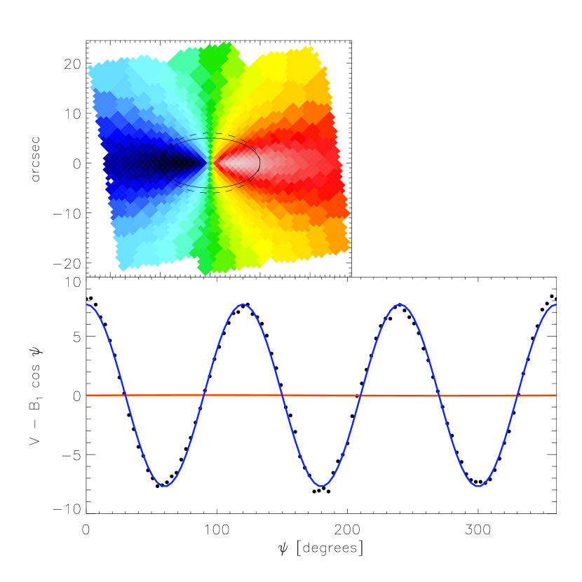
Figure 8: The effect of an incorrect flattening on the coefficients of harmonic expansion of a velocity profile. Upper panels shows the model velocity map having constant orientation (kinematic position angle) and flattening. The solid ellipse has correct flattening and orientation, while the dashed ellipse has incorrect axial ratio and correct orientation. The lower panel shows residuals between the extracted velocity profile and the circular velocity $B_{1}\cos(\psi)$ (solid symbols). Overplotted are contributions of $A_{1}\sin(\psi)$ (red line) and $B_{3}\cos(3\psi)$ (blue curve).

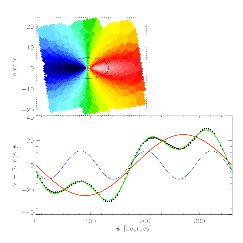
Figure 9: Same as Fig. 8 where the dashed ellipse has correct flattening but incorrect orientation. Next to the residuals on the lower panel overplotted are curves indicating the contribution of different terms: $A_{1}\sin(\psi)$ (red curve), $A_{3}\sin(3\psi)+B_{3}\cos(3\psi)$ (blue curve), and a combination $A_{1}\sin(\psi)+A_{3}\sin(3\psi)+B_{3}\cos(3\psi)$ (green curve).

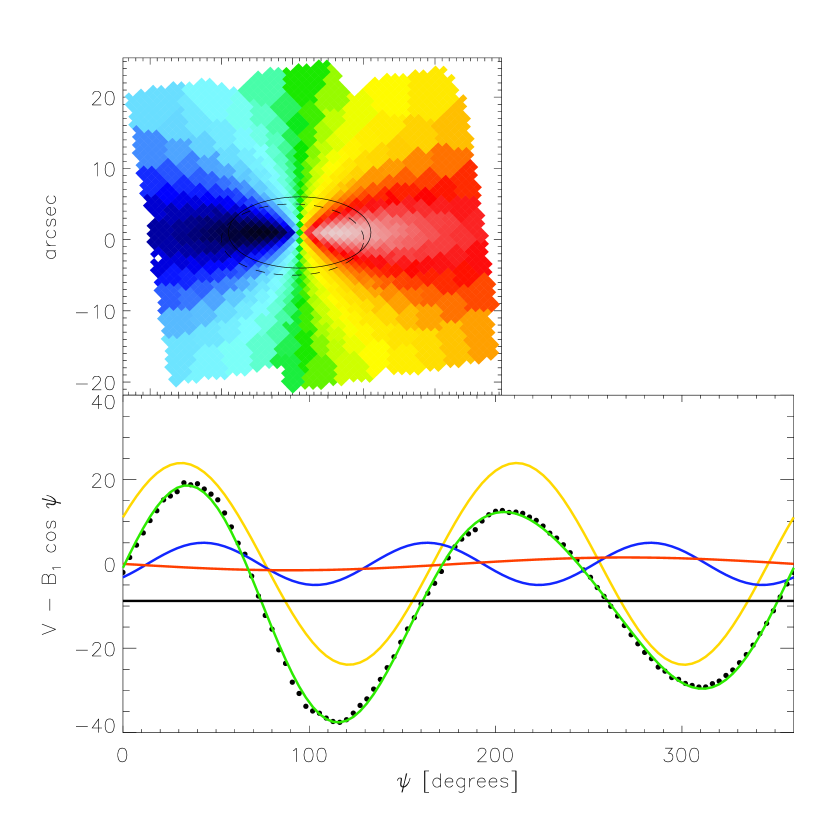
Figure 10: Same as Fig. 8 where the dashed ellipse of correct flattening and position angle was shifted by 1″horizontally and 1″vertically from the centre. The lower panel presents the residual and contributions from different terms: $A_{0}$ (black line), $A_{1}\sin\psi$ (red line), $A_{2}\sin(2\psi)+B_{2}\cos(2\psi)$ (orange curve) and $A_{3}\sin(3\psi)+B_{3}\cos(3\psi)$ (blue curve). The combined contribution of all these terms is overplotted with the green curve.

Here we test the sensitivity of harmonic expansion of a velocity profile given by eq. (3.2) with respect to a chosen incorrect flattening (inclination in a thin disk case), position angle and the centre of the ellipse along which the profile was extracted. We constructed a simple velocity map using the circular velocity form the Hernquist potential and an exponential light profile corresponding to the central (disk) component of the model 0. The velocity map had a constant flattening of $q_{0}=0.5$ and kinematic position angle of $\Gamma_{0}=0\degr$. Systemic velocity was set to zero. We first extracted a velocity profile from this map at $a=10\arcsec$ along a pre-designed ellipse. The ellipse was first chosen to have an incorrect flattening $q^{\prime}=0.6$, but correct kinematic position angle $\Gamma_{0}$ (Fig. 8). We repeated the exercise selecting the ellipse with incorrect $\Gamma^{\prime}=10\degr$ and correct $q$ (Fig. 9). Each of the profiles were then harmonically expanded with eq. (3.2). Finally, we shifted an ellipse, defined by correct values of $q$ and $\Gamma$, horizontally and vertically for 1″(Fig. 10). The corresponding velocity profile was expanded using first $N=6$ (even and odd) terms in eq. (6).

Harmonic expansion of a profile extracted along an ellipse defined by the correct centre, flattening and orientation would (by construction) yields all harmonic coefficients zero expect the $B_{1}$, which gives the circular velocity of the map. Hence, on the lower panels of Figs. 8, 9 and 10 we plot the difference (residuals) of the extracted velocity profile and the $B_{1}\cos(\psi)$ term.

On Fig. 8 overplotted are the contributions of terms: $A_{1}\sin(\psi)$ and $B_{3}\cos(3\psi)$. The $A_{3}\sin(3\psi)$ is nearly zero, like the $a_{1}$, and is not shown. The contribution of only the $B_{3}\cos(3\psi)$ term can explain the distribution of residuals, confirming that only $B_{3}$ coefficient is affected when choosing an incorrect flattening.

On Fig. 9 overplotted are the following terms: $A_{1}\sin(\psi)$, $A_{3}\sin(3\psi)+B_{3}\cos(3\psi)$, $B_{3}\cos(3\psi)$, as well as the combination $A_{1}\sin(\psi)+A_{3}\sin(3\psi)+B_{3}\cos(3\psi)$. All of these terms contribute significantly to describe the distribution of residuals. The dominant coefficient is $A_{1}$, while $A_{3}$ and $B_{3}$ contribute in this example with about 45% and 15% in amplitude, respectively. In the limit of a small incorrect position angle, Schoenmakers et al. (1997) showed that only $A_{1}$ and $A_{3}$ are affected, but our example shows that for larger incorrect position angles the $B_{3}$ term has to be considered as well.

Fig. 10 presents contributions for $A_{0}$, $A_{1}$, $A_{2}$, $B_{2}$, $A_{3}$ and $B_{3}$ harmonic terms. To the first order, only $A_{0}$, $A_{2}$ and $B_{2}$ terms are sensitive to incorrect centring. The same result was also analytically derived by Schoenmakers et al. (1997), in the limit of small miscentering. However, for large deviation from the true centre coordinates, contribution from the $A_{3}$ and $B_{3}$ terms becomes important, while $A_{1}$ remains much smaller.

We conclude this exercise by stating that the ellipse parameters for an odd kinematic moment map can determined by harmonic expansion of the $A_{0}$, $A_{1}$, $A_{2}$, $B_{2}$, $A_{3}$ and $B_{3}$ terms only.

Appendix C Determination of global kinematic position angle

The apparent angular momentum L_p of a galaxy, as a projection of the intrinsic angular momentum to the plane of sky, is defined as (Franx, 1988):

$$\mathbf{L_{p}}=\int_{P}\mathbf{r_{p}}\times\Sigma\mathbf{v_{r}}d\mathbf{r_{p}}$$ (13)

where $\mathbf{r{{}_{p}}}$ is a projection to the plane of sky of the vector $\mathbf{r}$ at which the mean velocity of stars, $\mathbf{v}$, projects to the observed radial velocity vector $\mathbf{v{{}_{r}}}$. $\Sigma$ is surface density and the integration is over the whole projection plane. As noted by Franx et al. (1991), it follows from eq. (13) that the apparent angular momentum is fully specified by the observed surface brightness and the observed two dimensional velocity map. In addition to that, if figure rotation is absent, the apparent angular momentum is parallel to the projection of the intrinsic angular momentum. This means that the projection of the full three-dimensional velocity space is reduced to the projection of the angular momentum. Reversing the argument, measuring the (luminosity weighted) kinematic position angle of the two-dimensional projection of velocities, it is possible to determine the position of the apparent angular momentum.

The position angle of the apparent angular momentum $\Gamma_{kin}$ can be determined from eq. (13) using integral-field observations of galaxies. This is the most physical way of determination of $\Gamma_{kin}$, but it is somewhat dependant on the geometry of the maps, like the relative orientation of the map with respect to the orientation of the apparent angular momentum.

A more robust way of determining $\Gamma_{kin}$ is based on a direct determination of the kinematic position angle $\Gamma$. Kinemetry measures $\Gamma$ as a function of radius, but we are interested in a global (independent of radius) value of the kinematic position angle, $\Gamma_{G}$, because of a direct correspondence between $\Gamma_{G}$ and $\Gamma_{kin}$. $\Gamma_{G}$ can be determined in a robust way using the information in the whole velocity map. For any chosen $\Gamma_{G}$, we construct a bi-anti-symmetric velocity map $V^{\prime}(x,y)$ with the $x$-axis along the given $\Gamma_{G}$. This is done by replacing the measured mean velocity $V(x,y)$ inside each Voronoi bin, of centroidal coordinates $(x,y)$, with the weighted average of the corresponding velocity in the four quadrants, using linear interpolation when needed to estimate the velocity:

$$V^{\prime}(x,y)=\frac{V(x,y)+V(x,-y)-V(-x,y)-V(-x,-y)}{4}$$ (14)

When any of the four symmetric coordinates was outside the convex hull defined by the bins centroids, we used only the remaining values to determined $V^{\prime}$. Fig. 11 shows an example of a bi-anti-symmetric map. The true $\Gamma_{G}$ was defined as the angle which minimises

$$\chi^{2}=\sum_{n=1}^{N}\left(\frac{V^{\prime}(x,y)-V(x,y)}{\Delta V(x,y)}\right)^{2}$$ (15)

In this way it is possible to assign simple error estimates to the obtained $\Gamma_{G}$ as the range of angles for which $\Delta\chi^{2}<9$, which corresponds to the $3\sigma$ confidence level for one parameter.

We used velocity maps from section 5.2 to compute the global kinematic position angle. Obtained values for NGC 2974, NGC 4459, NGC 2549 and NGC 4473 are 43.2, 280.6, 1.0, 92.5, respectively. The results are overplotted on Fig. 7 where they can be compared with the kinemetric position angle, $\Gamma$, which changes with radius describing specific features on the maps. They are in a very good agreement as can be seen comparing with the median values of the kinemetric position angle.

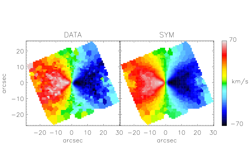
Figure 11: Comparison of observed velocity map (left) and bi-anti-symmetric map (right) at the best fitting $\Gamma_{G}$ using the method outlined in the text. We used SAURON observations of NGC 4473. North is up and east to the left.

References

- Arnold et al. (1994) Arnold R., de Zeeuw P. T., Hunter C., 1994, MNRAS, 271, 924
- Bacon et al. (2001) Bacon R., et al., 2001, MNRAS, 326, 23
- Begeman (1987) Begeman K. G., 1987, Ph.D. Thesis, Groningen University
- Bender (1988) Bender R., 1988, A&A, 193, L7
- Bender et al. (1988) Bender R., Doebereiner S., Moellenhoff C., 1988, A&AS, 74, 385
- Bender & Moellenhoff (1987) Bender R., Moellenhoff C., 1987, A&A, 177, 71
- Bender et al. (1994) Bender R., Saglia R. P., Gerhard O. E., 1994, MNRAS, 269, 785
- Bender et al. (1989) Bender R., Surma P., Doebereiner S., Moellenhoff C., Madejsky R., 1989, A&A, 217, 35
- Binney (1978) Binney J., 1978, MNRAS, 183, 779
- Binney & Tremaine (1987) Binney J., Tremaine S., 1987, Galactic dynamics. Princeton, NJ, Princeton University Press, 1987, 747 p.
- Busarello et al. (1992) Busarello G., Longo G., Feoli A., 1992, A&A, 262, 52
- Cappellari & Copin (2003) Cappellari M., Copin Y., 2003, MNRAS, 342, 345
- Cappellari & McDermid (2005) Cappellari M., McDermid R. M., 2005, Classical and Quantum Gravity, 22, 347
- Carter (1978) Carter D., 1978, MNRAS, 182, 797
- Copin (2002) Copin Y., 2002, in ASP Conf. Ser. 282: Galaxies: the Third Dimension Kinemetry: Quantifying Kinematic Maps. pp 508–+
- Copin et al. (2001) Copin Y., et al., 2001, in SF2A-2001: Semaine de l’Astrophysique Francaise Kinemetry: quantifying kinematic maps. p. 289
- Davies et al. (1983) Davies R. L., Efstathiou G., Fall S. M., Illingworth G., Schechter P. L., 1983, ApJ, 266, 41
- Davies & Illingworth (1983) Davies R. L., Illingworth G., 1983, ApJ, 266, 516
- Davis et al. (1985) Davis L. E., Cawson M., Davies R. L., Illingworth G., 1985, AJ, 90, 169
- de Zeeuw (1994) de Zeeuw P. T., 1994, in The Formation and Evolution of Galaxies; Structure, Dynamics and Formation of Spheroidal Systems. p. 231
- de Zeeuw et al. (2002) de Zeeuw P. T., et al., 2002, MNRAS, 329, 513
- Emsellem et al. (2004) Emsellem E., et al., 2004, MNRAS, 352, 721
- Emsellem et al. (1999) Emsellem E., Dejonghe H., Bacon R., 1999, MNRAS, 303, 495
- Emsellem et al. (2003) Emsellem E., Goudfrooij P., Ferruit P., 2003, MNRAS, 345, 1297
- Franx (1988) Franx M., 1988, Ph.D. Thesis, University of Leiden
- Franx et al. (1991) Franx M., Illingworth G., de Zeeuw P. T., 1991, ApJ, 383, 112
- Franx et al. (1989) Franx M., Illingworth G., Heckman T., 1989, AJ, 98, 538
- Franx et al. (1994) Franx M., van Gorkom J. H., de Zeeuw P. T., 1994, ApJ, 436, 642
- Gerhard (1993) Gerhard O. E., 1993, MNRAS, 265, 213
- Helfer et al. (2003) Helfer T. T., Thornley M. D., Regan M. W., Wong T., Sheth K., Vogel S. N., Blitz L., Bock D. C.-J., 2003, ApJS, 145, 259
- Hernandez et al. (2005) Hernandez O., Carignan C., Amram P., Chemin L., Daigle O., 2005, MNRAS, 360, 1201
- Hernquist (1990) Hernquist L., 1990, ApJ, 356, 359
- Hunter & Qian (1993) Hunter C., Qian E., 1993, MNRAS, 262, 401
- Jaffe et al. (1994) Jaffe W., Ford H. C., O’Connell R. W., van den Bosch F. C., Ferrarese L., 1994, AJ, 108, 1567
- Jedrzejewski (1987) Jedrzejewski R. I., 1987, MNRAS, 226, 747
- Kent (1983) Kent S. M., 1983, ApJ, 266, 562
- Kent (1984) Kent S. M., 1984, ApJS, 56, 105
- Kormendy & Bender (1996) Kormendy J., Bender R., 1996, ApJ, 464, L119+
- Krajnović et al. (2005) Krajnović D., Cappellari M., Emsellem E., McDermid R. M., de Zeeuw P. T., 2005, MNRAS, 357, 1113
- Krajnović (2004) Krajnović D., 2004, Ph.D. Thesis, University of Leiden
- Lauer (1985a) Lauer T. R., 1985a, MNRAS, 216, 429
- Lauer (1985b) Lauer T. R., 1985b, ApJS, 57, 473
- Lauer et al. (1995) Lauer T. R., et al., 1995, AJ, 110, 2622
- Moré et al. (1980) Moré J. J., Garbow B. S., Hillstrom K. E., 1980, User Guide for MINPACK-1, Argonne National Laboratory Report ANL-80-74, 74
- Nieto & Bender (1989) Nieto J.-L., Bender R., 1989, A&A, 215, 266
- Nieto et al. (1988) Nieto J.-L., Capaccioli M., Held E. V., 1988, A&A, 195, L1
- Peletier et al. (1990) Peletier R. F., Davies R. L., Illingworth G. D., Davis L. E., Cawson M., 1990, AJ, 100, 1091
- Press et al. (1992) Press W. H., Teukolsky S. A., Vetterling W. T., Flannery B. P., 1992, Numerical recipes in FORTRAN. The art of scientific computing. Cambridge: University Press, —c1992, 2nd ed.
- Rest et al. (2001) Rest A., van den Bosch F. C., Jaffe W., Tran H., Tsvetanov Z., Ford H. C., Davies J., Schafer J., 2001, AJ, 121, 2431
- Schoenmakers et al. (1997) Schoenmakers R. H. M., Franx M., de Zeeuw P. T., 1997, MNRAS, 292, 349
- Statler (1991) Statler T. S., 1991, AJ, 102, 882
- Statler (1994a) Statler T. S., 1994a, ApJ, 425, 458
- Statler (1994b) Statler T. S., 1994b, ApJ, 425, 500
- Statler & Fry (1994) Statler T. S., Fry A. M., 1994, ApJ, 425, 481
- Swaters et al. (2002) Swaters R. A., van Albada T. S., van der Hulst J. M., Sancisi R., 2002, A&A, 390, 829
- Teuben (1991) Teuben P. J., 1991, in Warped Disks and Inclined Rings around Galaxies, eds S. Casertano, P.D. Sackett & F.H. Briggs, (Cambridge Univ. Press) Velocity Fields of Disks in Triaxial Potentials. p. 40
- van der Marel & Franx (1993) van der Marel R. P., Franx M., 1993, ApJ, 407, 525
- Wagner et al. (1988) Wagner S. J., Bender R., Moellenhoff C., 1988, A&A, 195, L5
- Wong et al. (2004) Wong T., Blitz L., Bosma A., 2004, ApJ, 605, 183