Mass loss and orbital period decrease in detached chromospherically active binaries

Abstract

The secular evolution of the orbital angular momentum (OAM), the systemic mass $(M=M_{1}+M_{2})$ and the orbital period of 114 chromospherically active binaries (CABs) were investigated after determining the kinematical ages of the sub-samples which were set according to OAM bins. OAMs, systemic masses and orbital periods were shown to be decreasing by the kinematical ages. The first order decreasing rates of OAM, systemic mass and orbital period have been determined as $\dot{J}=3.48\times 10^{-10}~{}yr^{-1}$ per systemic OAM, $\dot{M}=1.30\times 10^{-10}~{}yr^{-1}$ per systemic mass and $\dot{P}=3.96\times 10^{-10}~{}yr^{-1}$ per orbital period respectively from the kinematical ages. The ratio of $d\log J/d\log M=2.68$, which were derived from the kinematics of the present sample, implies that there must be a mechanism which amplifies the angular momentum loss $\bar{A}=2.68$ times in comparison to isotropic angular momentum loss of hypothetical isotropic wind from the components. It has been shown that simple isotropic mass loss from the surface of a component or both components would increase the orbital period.

1 Introduction

The observational evidence of decaying rotation rate for stars with spectral types later than F in the stellar evolution was well documented by Skumanich (1972) by studying projected equatorial speeds $(v\sin i)$ of the late-type stars in open clusters of different ages. Such a decay process in stellar rotation is explained in the terms of angular momentum loss (AML) through magnetically driven stellar winds, also called the magnetic braking (cf. Schatzman 1959, Kraft 1967 and Mestel 1968). For the tidally locked binaries with late-type components, such an AML is known to be provided by the reservoir of the orbital angular momentum (OAM). Therefore, the AML from the components of spin-orbit coupled binaries causes the orbit to shrink. Spin-orbit coupling and a shrinking orbit, then, imposes spin-up the rotation of the components, which is different from single stars slowing down rotation. This mechanism is considered as the main way to form W UMa-type contact binaries from systems initially detached (cf. Huang 1966, Okamoto & Sato 1970, van’t Veer 1979, Vilhu & Rahunen 1980, Mestel 1984, Guinan & Bradstreet 1988, Maceroni & van’t Veer 1991, Stepien 1995, Demircan 1999).

The period evolution and the time scale of forming the contact binaries from the detached progenitors were estimated differently among the various authors. In the work of Guinan & Bradstreet (1988), the AML of a component star was computed directly from Skumanich’s law ($V_{rot}\sim t^{1/2}$), which is derived from the relatively slow rotating stars ($V_{rot}\leq 17$ km s^-1), and then AML from the two components made equal to the orbital AM change. Orbits evolve initially almost with constant periods until the very end where the orbits shrink sharply to form contact binaries. For the braking law of binary orbits, van’t Veer & Maceroni (1988, 1989) gave a period evolution function which was predicted from the initial (Abt & Levy 1976, Abt 1983) and the present day (Farinella et al. 1979) period distributions of G-type binaries corrected for selection and detectability effects. Stepien (1995) derived a formula with no free parameters for the AML via a magnetized wind and calibrated it from the spin down of single stars. He concludes that usually the orbital periods which are less than 5 days can form contact systems within their main-sequence lifetime.

What is common among those works is the spin-orbit coupling set by synchronization. In other words, the above mechanisms do not work for asynchronous binaries as van’t Veer & Maceroni (1988) stated that the wider systems without spin-orbit coupling will not change the orbital period. Therefore, Demircan (1999) studied the orbital AM distribution of 40 well-known CABs only with $P_{orb}<10$ days, and found an observational estimate of the rate of orbital AML and the braking law from the upper boundary of the orbital AM distribution.

Usage of small number statistics and saturation in activity-rotation relation may be responsible for the weakness among those studies. Perhaps, the upper boundary does not represent all systems, and the mass loss and the AML may be age-dependent quantities. In order to better understand the orbital period evolution of detached active binaries, systems with different ages should be considered. Although the ages of binaries can be estimated only by detailed evolutionary isochrones, the sub-group ages can be found kinematically. Recently, after having more accurate data on a large sample of detached CABs, Karataş et al. (2004) became successful in breaking up the sample into kinematically distinct sub-samples. Karataş et al. (2004) initially divided the whole sample of 237 systems into two groups: the possible moving group (MG) members (95) and the older field binaries (142). A comparison of the total mass, the orbital period, the mass ratio and the orbital eccentricity of these two groups revealed clear observational evidence that detached CABs lose mass and angular momentum so that their orbits circularize and shrink. Related orbital period decreases, unfortunately, are not detectable on commonly used O–C diagrams formed by the eclipse minimum times. This is due to: 1) very short time span covered by existing O–C data (at most 100 years) in comparison with durations implied by the predicted kinematical ages which are at the order of $10^{9}$ years; 2) large scatter of unevenly distributed data (especially visual and photographic observations) in the present O–C diagrams; 3) existence of complicated larger amplitude short time scale fluctuations caused by many different effects (cf Kreiner, Kim & Nha 2001; Demircan 2000, 2002). Being independent of the physical cause, the O–C diagrams are commonly used in the study of orbital period changes of binaries in general. At present, mean minimum time deviations as small as 10 seconds for binaries with sharp eclipses are detectable. Nevertheless, the minimum detectable period variation on O–C diagrams depends on the time span of observations over the actual variations.

This classical approach with O–C diagrams, thus, are not suitable to obtain slower secular orbital decreases implied by the wind driven mass loss of our sample of detached CABs. Consequently, our aim in the present work is to further investigate the mass-loss, the angular momentum loss, orbital period decrease and then determine the rates of change of those parameters statistically from the new and more accurate data (absolute dimensions and kinematical data) of Karataş et al. (2004). The present approach, apparently, is more advantageous in detecting changes at the order of evolutionary time scales, where O–C diagrams becomes insufficient, and also more practical to give no distinction weather the involved binaries are eclipsing or not.

2 data

Among the total 237 CABs studied kinematically by Karataş et al. (2004), 119 systems with complete basic data (orbital and physical), which allows computation of orbital angular momentum $J$, were selected for this study. Although, contact (W UMa) and semi-contact ($\beta$ Lyrea and classical Algols) systems were intentionally excluded from the catalog of chromospherically active binary stars (CAB, Strassmeier et al. 1988, 1993), thus, CABs are known to be detached systems. Nevertheless, the catalog still contains small number of systems like $\epsilon$ UMi (de Medeiros & Udry 1999), RT Lac (Heunemoerder & Barden 1986; Popper 1991), RV Lib (Popper 1991), BH CVn (Eker 1987), RZ Cnc (Olson 1989), AP Psc (Eaton & Barden 1988) and AR Mon (Williamon et al. 2005) with a component filling or about to fill its Roche lobe that mass transfer possibly exist. Since we are interested in only detached active binaries, five of such systems (BH CVn, RT Lac, RV Lib, AR Mon and $\epsilon$ UMi), were further discarded from our final list that our sample reduced to 114 systems.

62 out of 114 are in the sub-sample (142 binaries) which were called the field stars. Karataş et al. (2004) assigned an age 3.86 Gyr to this group from the galactic space velocity components. This group is a mixture of young and old stars together. Therefore, the assigned age does not represent each system individually. It is an average age suggested by their kinematics. The 62 field stars and their data are displayed in Table 1. Columns are order number, name, HD number, orbital period, rotational period of the most active star, total mass ($M=M_{1}+M_{2}$), mass ratio ($q=M_{2}/M_{1}<1$), logarithm of the orbital angular momentum and assigned kinematical age. How these ages were assigned will be explained in Section 3.2.

Those field binaries have been further divided in five groups according to OAM but displayed as sorted on orbital periods. The groups are shown as separated by a blank row in Table 1.

Table 1: Physical parameters of the field CABs.

No	Name	HD	$P_{orb}$	$P_{rot}$	$M_{tot}$	$q$	$\log J$	Age
			(days)	(days)	$(M_{\odot})$		(cgs)	(Gyr)
1	XY UMa	237786	0.479		3.58	0.954	51.76	9.16
2	BI Cet	8358	0.516	0.520	1.84	0.957	51.84	9.16
3	SV Cam	44982	0.593	0.593	1.37	0.957	51.81	9.16
4	WY Cnc		0.829	0.829	2.82	0.958	51.75	9.16
5	CM Dra		1.268	1.268	2.75	0.833	50.94	9.16
6	CC Eri	16157	1.562	1.561	1.44	0.675	51.42	9.16
7	EI Eri	26337	1.947	1.945	1.18	0.269	51.63	9.16
8	BK Psc		2.166		1.50	0.974	51.59	9.16
9	V1396 Cyg		3.276		0.66	0.696	51.35	9.16
10	HZ Aqr		3.757		1.23	0.804	51.83	9.16
11	UZ Lib		4.768	4.736	1.54	0.921	51.84	9.16
12	BY Dra	234677	5.975		5.09	0.951	51.70	9.16
13	LR Hya	91816	6.866	3.145	2.91	0.942	51.83	9.16
14	II Peg	224085	6.724	6.718	1.20	0.500	51.85	9.16
15	OU Gem	45088	6.992	7.360	1.43	0.700	51.89	9.16
16	UV Leo	92109	0.600		3.06	0.951	51.99	6.57
17	BH Vir	121909	0.817	0.817	3.53	0.604	51.97	6.57
18	V837 Tau	22403	1.930	1.890	2.12	0.909	51.94	6.57
19	AR Lac	210334	1.983	1.983	2.39	0.897	52.22	6.57
20	CF Tuc	5303	2.798	2.798	1.75	0.865	52.23	6.57
21	AD Cap	206046	2.960	2.960	1.62	0.526	51.96	6.57
22	AS Dra	107760	5.413	5.413	2.54	0.906	51.99	6.57
23	V1423 Aql	191262	5.434	5.530	1.85	0.682	52.25	6.57
24	KT Peg	222317	6.202	6.092	1.54	0.671	52.05	6.57
24	UV CrB	136901	18.667		4.10	0.464	52.04	6.57
26	V711 Tau	22468	2.838	2.841	1.85	0.993	52.31	4.07
27	PW Her		2.881	2.881	2.50	0.786	52.34	4.07
28	TY Pyx	77137	3.199	3.320	2.22	0.947	52.30	4.07
29	SAO 240653	114630	4.233		3.25	0.979	52.26	4.07
30	UX Ari	21242	6.438	6.438	2.19	0.975	52.28	4.07
31	SS Boo		7.606	7.606	1.04	0.951	52.26	4.07
32	EZ Peg		11.660	11.663	1.86	0.991	52.30	4.07
33	AR Psc	8357	14.302	12.245	1.63	0.567	52.39	4.07
34	V350 Lac	213389	17.753		1.80	0.818	52.33	4.07
35	FG UMa	89546	21.360		2.83	0.991	52.37	4.07
36	XX Tri	12545	23.969	24.300	1.67	0.964	52.30	4.07
37	SZ Psc	219113	3.965	3.955	2.86	0.766	52.44	2.95
38	Z Her	163930	3.993	3.962	1.99	0.881	52.45	2.95
39	RS UMi		6.169		3.09	0.818	52.41	2.95
40	MM Her	341475	7.960	7.936	1.70	0.546	52.45	2.95
41	FF Aqr		9.208	9.208	3.10	0.240	52.43	2.95
42	42 Cap	206301	13.174		2.37	0.727	52.48	2.95
43	IS Vir	113816	23.655		0.62	0.938	52.44	2.95
44	AI Phe	6980	24.590		1.19	0.924	52.60	2.95
45	IM Peg	216489	24.649	24.390	2.30	0.533	52.52	2.95
46	TW Lep	37847	28.344	28.220	2.78	0.704	52.47	2.95
47	V4200 Ser	188088	46.817	16.500	4.93	0.904	52.43	2.95
48	EL Eri	19754	48.263	47.960	0.50	0.917	52.43	2.95
49	AY Cet	7672	56.824	77.220	1.75	0.765	52.60	2.95
50	V1197 Ori	38099	143.040		1.29	0.949	52.55	2.95
51	RU Cnc		10.173	10.135	2.23	0.855	52.61	2.55
52	CQ Aur	250810	10.623	10.560	1.83	0.564	52.79	2.55
53	TZ Tri	13480	14.729	14.729	2.73	0.365	53.06	2.55
54	$\zeta$ And	4502	17.769		2.14	0.739	52.65	2.55
55	BL CVn	115781	18.692	18.692	0.57	0.979	52.63	2.55
56	CS Cet	6628	27.322		2.15	0.957	52.71	2.55
57	V792 Her	155638	27.538	27.070	4.50	0.800	52.74	2.55
59	V1762 Cyg	179094	28.590	28.590	7.73	0.600	52.72	2.55
59	V965 Sco	158393	30.969	30.960	3.95	0.879	52.88	2.55
60	RZ Eri	30050	39.282	31.400	1.10	0.970	52.89	2.55
61	DK Dra	106677	64.474	63.750	2.55	0.930	53.00	2.55
62	BD+44 801	23838	962.800		0.68	0.545	53.22	2.55

Table 2: Physical parameters of the MG CABs.

No	Name	HD	$P_{orb}$	$P_{rot}$	$M_{tot}$	$q$	$\log J$	MG	OC	Age
			(days)	(days)	$(M_{\odot})$		(cgs)			(Gyr)
1	V471 Tau		0.521	0.597	1.50	0.974	51.69	Hya	Hya	0.6
2	RT And		0.629	0.629	2.14	0.739	51.97	UMa		0.3
3	CG Cyg		0.631	0.631	1.75	0.865	51.83	UMa		0.3
4	ER Vul	200391	0.698	0.694	2.15	0.957	51.99	IC		0.055
5	YY Gem	60179	0.814	0.814	1.19	0.924	51.59	Cas		0.20
6	UV Psc	7700	0.861	0.861	1.75	0.765	51.87	IC		0.055
7	V1430 Aql		0.874		1.84	0.957	51.91	LA		0.15
8	V772 Her	165590	0.880	0.878	1.63	0.567	51.79	LA		0.15
9	IL Com	108102	0.962	0.820	1.67	0.964	51.86	Cas	Com Ber	0.20
10	$\delta$ Cap	207098	1.023		2.73	0.365	52.12	LA		0.15
11	DH Leo	86590	1.070	1.066	1.44	0.675	51.75	Hya, IC		0.6
12	Gl 841A		1.123		0.50	0.917	51.01	LA		0.15
13	TZ CrB	146361	1.140	1.169	2.19	0.975	52.08	LA		0.15
14	BD+23 2297	95559	1.526	1.526	1.85	0.993	52.00	Hya, IC		0.6
15	V824 Ara	155555	1.682	1.682	2.12	0.909	52.11	LA		0.15
16	13 Cet	3196	2.082		0.68	0.545	51.28	Hya		0.6
17	V478 Lyr	178450	2.131	2.131	1.18	0.269	51.55	IC		0.055
18	FF And		2.170	2.170	1.10	0.970	51.67	IC		0.055
19	KZ And	218738	3.033	3.030	1.29	0.949	51.84	Cas, IC		0.2
20	BD+39 4529	203454	3.243		1.83	0.564	52.06	UMa		0.3
21	V835 Her	163621	3.304	3.350	1.43	0.700	51.91	LA		0.15
22	HZ Com		3.558		1.37	0.957	51.90	Cas	Com Ber	0.2
23	GK Hya		3.587	3.587	2.56	0.910	52.36	Hya		0.6
24	UX Com		3.642	3.642	2.23	0.855	52.26	Hya		0.6
25	BU 163	202908	3.966		2.22	0.947	52.27	UMa		0.3
26	RS CVn	114519	4.798	4.791	2.82	0.958	52.47	IC		0.055
27	SS Cam		4.824	4.823	3.58	0.954	52.64	LA		0.15
28	RT CrB	139588	5.117	5.117	2.83	0.991	52.48	UMa		0.3
29	VV Mon		6.051	6.051	2.91	0.942	52.53	IC		0.055
30	RW UMa		7.328	7.328	3.06	0.951	52.59	IC		0.055
31	LX Per		8.038	7.905	2.55	0.930	52.47	Hya	$\alpha$ Per	0.6
32	AW Her	348635	8.801		2.54	0.906	52.48	Hya		0.6
33	V1285 Aql		10.319	2.900	0.62	0.938	51.48	Cas		0.2
34	AE Lyn	65626	11.068	10.163	3.25	0.979	52.69	IC		0.055
35	V829 Cen	101309	11.710	11.660	0.57	0.979	51.45	Cas		0.2
36	V808 Tau	283882	11.929	6.820	1.58	0.950	52.18	Hya	Hya	0.6
37	IL Hya	81410	12.905	12.890	3.53	0.604	52.75	UMa		0.3
38	V1379 Aql	185510	20.661	25.640	3.05	0.129	52.34	LA		0.15
39	ADS11060C	165590C	25.763	9.000	1.04	0.951	51.99	LA		0.15
40	BD+64 487	30957	44.396		1.54	0.921	52.35	Cas, IC		0.2
41	KX Peg	212280	45.284	29.060	3.09	0.818	52.86	UMa		0.3
42	BD+44 2760	161570	45.623		2.75	0.833	52.77	IC		0.055
43	GT Mus	101379	61.360	56.030	4.50	0.800	53.17	LA		0.15
44	DQ Leo	102509	71.690	55.000	3.95	0.879	53.10	Hya		0.6
45	BD+17 703	27149	75.648		1.99	0.881	52.62	Hya	Hya	0.6
46	BM Cam	32357	80.898	85.000	1.70	0.546	52.47	LA		0.15
47	5 Cet	352	96.400	96.320	2.50	0.786	52.81	Cas		0.2
48	$\alpha$ Aur	34029	104.023	80.000	5.09	0.951	53.34	Hya		0.6
49	V1817 Cyg	184398	108.854	108.854	7.73	0.600	53.62	UMa		0.3
50	$\eta$ And	5516	115.720		4.93	0.904	53.33	UMa		0.3
51	SAO 23511	57853	122.169		1.85	0.682	52.62	IC		0.055
52	V819 Her	157482	2018.000	81.900	2.78	0.704	53.32	UMa		0.3

The rest, 52 systems out of 114, are in the sub-sample which were called MG. Kinematical criteria originally defined by Eggen (1958a, b, 1989, 1995), for determining possible members of the best-documented moving groups, are summarized by Montes et al. (2001a, b). One may see Karataş et al. (2004) for details as to how MG systems were selected from the common CABs. However, the basic idea is that a test star’s space velocity vector must be equal and parallel, or at least with deviations smaller than pre-determined limits, to the space velocity vector of a moving group. The ages of moving groups are known as open cluster ages by the turn-off point from the main sequence. Consequently, a pre-determined age of a moving group can be assigned to all binaries which are found to be possible members according to their space velocity vectors. Therefore, unlike the field stars with various ages, the MG stars are homogeneous with a single age corresponding to each MG. Among the five MG considered by Karataş et al. (2004), the Hyades Supercluster is the oldest one with 0.6 Gyr age (see Table 3 of Karataş et al. 2004). The 52 systems and their assigned ages are listed in Table 2 in order of orbital period length. The columns are same as Table 1 but two more columns, name of the MG and associated open cluster, were inserted before the ages according to identified MG.

3 OAM evolution among the detached CABs

3.1 Basics of mass loss and OAM change

Assuming component masses as points, the OAM of a binary is given by the well known relation

$$J={M_{1}M_{2}\overwithdelims( )M_{1}+M_{2}}{a^{2}\Omega}={q\overwithdelims( )(1+q)^{2}}{Ma^{2}\Omega},$$ (1)

where

$${M_{1}M_{2}\overwithdelims( )M_{1}+M_{2}}{a^{2}}={q\overwithdelims( )(1+q)^{2}}{Ma^{2}}=I$$ (2)

is the moment of inertia and $\Omega=2\pi/P$ is the angular velocity of the system. $P$ is the orbital period, $M=M_{1}+M_{2}$ is the total mass, $q=M_{2}/M_{1}<1$ is the mass ratio of the components and $a$ is the semi major axis of the binary. Therefore, an isotropic mass loss from the surfaces of components will produce an OAM loss as

$$dJ={q\overwithdelims( )(1+q)^{2}}{a^{2}\Omega dM},$$ (3)

which might be due to isotropic stellar winds from one or both components under the condition that there must be no interaction between the winds nor between the winds and the components. Binaries are dynamical systems obeying Kepler’s third law. Therefore, the orbit re-arranges itself. Thus, the basic parameters ($a$, $M$ and $P$) must all change according to

$$3{da\over a}+2{d\Omega\over\Omega}={dM\over M}.$$ (4)

Consequently, the OAM change must provide their changes as

$${dJ\over J}={dM\over M}+2{da\over a}+{d\Omega\over\Omega}$$ (5)

according to (1), where the contribution of mass ratio change ($dq$) is neglected in the first approximation. If ${da\over a}$ is eliminated between (4) and (5), then

$${dJ\over J}={5\over 3}{dM\over M}-{1\over 3}{d\Omega\over\ \Omega}={5\over 3}{dM\over M}+{1\over 3}{dP\over P}$$ (6)

is obtained. But if $d\Omega\over\ \Omega$ is eliminated between (4) and (5),

$${dJ\over J}={3\over 2}{dM\over M}+{1\over 2}{da\over a}$$ (7)

is obtained. In another words, OAM change provides two independent equations which tell us how OAM is shared among the two parameters, $M$ and $P$ in one case, $M$ and $a$ in the other case, where the change in the missing parameter is provided by Kepler’s third law (eq. 4).

According to (1) and (3), the isotropic mass loss from surfaces implies

$${dJ\over J}={dM\over M},$$ (8)

which means the change in OAM has only one source: the mass loss, which were assumed to be isotropic. In order to see how the orbit reacts to this OAM change, it is plugged into eq. (6). Then, it gives us

$${dM\over M}=-{1\over 2}{dP\over P},$$ (9)

which means the orbital period must increase since negative $dM$ makes $dP$ positive. But, if it is plugged into eq. (7), it gives us

$${dM\over M}=-{da\over a},$$ (10)

which means the semi-major axis of the binary must increase similarly because negative $dM$ makes $da$ positive. A similar conclusion is given by Pringle (1985) who assumed isotropic non-interacting mass loss from one component only. Here, the problem is generalized. It does not matter whether one or both components lose mass, the result is the same; simple mass loss from the surfaces of components will cause the orbital period to increase rather than to decrease. Despite this, the system loses OAM. If a binary does not lose mass, the total angular momentum (orbital plus spin angular momentums) of the system is conserved. Therefore, for a system to lose angular momentum, mass loss is inevitable. However, eq. (8) tells us that ${dJ\over J}={dM\over M}$, that is, each particle leaving the system carries away an OAM which is equal to mean orbital angular momentum per mass in the system. There can be various mechanisms which can amplify angular momentum loss per particle leaving the system with respect to mean OAM per mass in the system. Consequently we define an amplification parameter $\bar{A}$ as

$${\bar{A}}={{dJ\over dM}\over{J\over M}}\Rightarrow{dJ\over J}={\bar{A}}{dM\over M},$$ (11)

where ${\bar{A}}$ is the ratio between angular momentum loss per mass and mean orbital angular momentum per mass in the system. Notice that ${\bar{A}}=1$ for isotropic mass loss from the surface of one or both components; then equation (11) reduces to be eq. (8). Inserting (11) into (6), we can write

$${(3\bar{A}-5)}{dM\over M}={dP\over P}.$$ (12)

From above, we can set up a condition $\bar{A}>5/3$ for a system to decrease its orbital period if orbital period decrease is due to OAM loss. Notice that mass loss is inevitable and the definition of ${\bar{A}}$ is meaningful only if $dM\neq 0$. Our sample CABs are all detached systems. Mass transfer must not be occurring. Nevertheless, mass loss too may produce mass ratio change, which we prefer to ignore for simplicity in the first approximation. Then, the orbital period evolution of detached CABs primarily depends on mass loss rate and the value of ${\bar{A}}$. Consequently, OAM evolution because of mass loss, needs to be understood first.

3.2 OAM evolution for detached field CABs

A more direct way of understanding OAM ($J$), orbital period and total mass evolution of CABs is provided by the kinematical ages of the sub-groups of the sample binaries. Although, the initial orbital periods and the initial masses are not known, the present orbital periods are confirmed to be shifted towards shorter periods by the increased ages of the subgroups according to orbital periods (see Fig. 7 of Karataş et al. 2004). In order to investigate the age dependence of the OAM ($J$), the orbital period ($P$) and the systemic total mass $M$ here, we have formed different sub-groups according to $J$ among the field detached CABs. Those sub-groups according to $J$ are separated by blank rows in Table 1. The mean orbital periods and the mean total mass of binaries in those sub-groups of the 62 field CABs are listed in Table 3. N in column 4 indicates the number of systems in each sub-group.

The kinematical ages of those sub-groups were determined from their space velocity dispersions, using the kinematical tables of Wielen (1982). The dispersions and the implied kinematical ages are listed in the last two columns of Table 3, together with their estimated standard errors. The mean $\log J$ and the kinematical ages of the sub-groups are plotted in Fig. 1. In the first approximation, a linear trend line was fitted using the least squares method. A linear trend line with a negative inclination in a logarithmic scale indicates an exponential decrease of OAM according to age. This is an observational evidence of OAM evolution provided by kinematical data.

The MG group binaries (Table 2), all have ages less than 0.6 Gyr, would have been shown by a vertical line in Fig. 1 for comparison to the field systems. Notice that the age is known for each star in a MG according to its moving group membership. Instead of expressing them by a vertical line, which would indicate no observable evolution, we have preferred to combine the field and MG systems, that is, re-arrange the total sample into six sub-groups according to their OAM ($J$). In this way we expected to see the effect of mixing young stars erroneously into the field systems. In other words: what would happen if MG systems were not selected out of a sample?

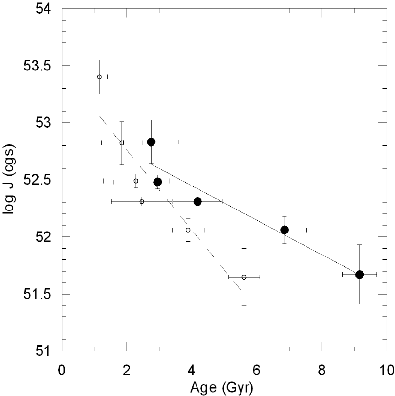
Figure 1: Orbital angular momentum $J$ versus age for the 62 field CABs (solid line) and whole sample (dashed line) of 114 stars.

Table 3: The sub-groups of the 62 field CABs according to OAM.

$\log J$	$<\log P>$	$<\log M>$	N	$\sigma_{tot}$	Age
(cgs)	(days)	$(M_{\odot})$		(km $s^{-1}$)	(Gyr)
(50.90, 51.90]	0.337	0.055	15	75.49   3.14	9.16   0.53
(51.90, 52.25]	0.472	0.259	10	62.24   3.75	6.85   0.67
(52.25, 52.40]	0.901	0.331	11	47.65   4.21	4.18   0.77
(52.40, 52.60]	1.275	0.364	14	40.56   8.16	2.95   1.34
(52.60, 53.25]	1.495	0.509	12	39.40   5.00	2.75   0.86

The kinematical ages of the six sub-groups of the total sample (MG+Field) have been re-computed from their space velocity dispersions as was done for the field stars. The assigned ages of MG systems in each group is ignored in this process. The kinematical ages and mean OAMs of these newly formed sub-groups are shown for comparison in Fig. 1 together with a line (dashed) fitted using the least squares method. The steeper inclination of the dashed line in Fig. 1 indicates there is faster OAM evolution among the total sample (114) in comparison to the evolution (solid line) within the field CABs. Of course, faster evolution is just an illusion because each sub-group of the total sample contains young stars with small space velocities with respect to LSR (Local Standard of Rest). Therefore, the mean dispersions of the total sample sub-groups are reduced. Smaller dispersions, on the other hand, correspond to smaller kinematical ages. With smaller ages, the higher inclination were produced. Accordingly, it can be concluded that the rate of decrease of OAM would be overestimated if young MG group stars were left in the sub-groups. Therefore, we conclude that the sub-groups in Table 3 are corrected for this error. As a result, the solid line in Fig. 1 shows the corrected OAM evolution among the CABs.

Nevertheless, this correction associated with removing possible MG members from a sample is still a first order correction. This is because the kinematical criteria for determining the moving group members do not constitute proof of membership since there is always a possibility that members and non-members could share the same velocity space. Karataş et al. (2004) believed non-members are negligible in number and do not spoil the statistics. Therefore, further purification by selecting out non members from the possible MG members, which requires independent proof of a different age or chemical composition, was not attempted. Since it is possible that some small number of field stars were erroneously selected as MG members, the inclination of the solid line in Fig. 1 can be considered a lower limit. This is because, if erroneously selected MG stars with smaller space velocity were put back into field stars, the ages of the sub-groups would have been lowered accordingly. Because this second order correction was not applied, we can only estimate that the OAM evolution among the field CABs could be little faster, but not slower than the evolution implied in Fig. 1.

3.3 Orbital period evolution and mass loss for detached field CABs

The observed OAM decrease among the field CABs requires mass loss to carry OAM out of the systems in order to have a reducing effect on the orbital periods unless there are mechanisms which do not require mass loss. One possibility is the direct loss of binary binding energy by stellar encounters in the galactic space which is expected to be effective down to few days period (Stepien  1995; Ghez, Neugebauer & Matthews 1993). Likely it is negligible, but the other possibility is friction between the binary components and circum binary material in Keplerian orbits. It is not the scope of this study to solve which mechanism is dominant and what are the contributions to the orbital period evolution. Indeed, the statistics in Table 3 clearly indicate that total masses and orbital periods also decrease with stellar kinematical ages similar to OAM evolution. The age dependence of the orbital periods $(P)$ and mean total masses $(M=M_{1}+M_{2})$ of the field CABs are plotted in Fig. 2, where the age dependence of $J$ is also shown for a comparison.

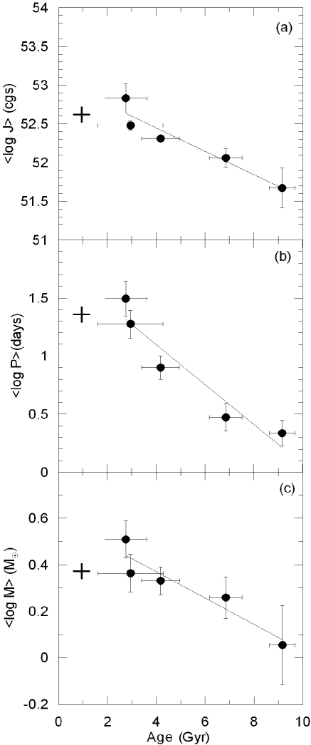
Figure 2: The age dependent variations of OAM $J$ (a), period $P$ (b) and mass $M$ (c) for the sub-groups of the 62 field CABs. Dot and plus show field and MG CABs, respectively.

The linear trend lines fitted by least squares indicate the first order approximations to describe the changes at $P$, $M$ and $J$. With similar arguments stated for $J$, the decreasing rates of systemic masses ($M$) and orbital periods ($P$) could also be considered as lower limits.

With ages less than 0.6 Gyr, the MG group CABs are plotted as a youngest group in Fig. 2. It is possible to claim that their position does not support the general trend of the fitted lines reasonably as their position appears lower than the position expected. This again could be explained by the pollution of a limited number of older stars in MG. The true members of MG would have agreed the general trends.

Orbital period data in Fig. 2b indicate that the orbital period changes $(dP/dt)$ at the younger ages are faster. Such a trend, however, will not be consistent with the orbital period shrinkage being slow at the beginning and becoming fast later as described by Guinan & Bradstreet (1988), van’t Veer & Maceroni (1988, 1989), Stepien (1995) and Demircan (1999) who predicted it from the magnetic braking of tidally locked close binaries. Nevertheless, the appearance of our data could be a result of small-number statistics so that we are content to assume the inclination is monotonic to the first approximation.

3.4 Decreasing rates for $J$, $P$ and $M$

Regression analysis of linear line fitting to the $J$, $P$ and $M$ data (Table 3) by least squares gives the following:

$$\log J=-(1.51\pm 0.27)\times 10^{-10}t+53.05\pm 0.13$$ (13)

$$\log P=-(1.72\pm 0.30)\times 10^{-10}t+1.79\pm 0.18$$ (14)

$$\log M=-(5.65\pm 1.18)\times 10^{-11}t+0.60\pm 0.07.$$ (15)

Taking the time derivatives,

$$dJ/dt=-3.48\times 10^{-10}J$$ (16)

$$dP/dt=-3.96\times 10^{-10}P$$ (17)

$$dM/dt=-1.30\times 10^{-10}M$$ (18)

are obtained for the detached field systems, where $J$ is in cgs, $t$ in yrs, $P$ in days and $M$ in $M_{\odot}$. As a natural consequence of a logarithmic scale, the derivatives are proportional to the varying function itself. Defining the decreasing rate coefficients as $\alpha_{X}=-{dx\overwithdelims( )dt}{1\overwithdelims( )X}$, where X could be $J$, $P$ or $M$, the rate coefficients for the orbital angular momentum, for the orbital period and for the total mass will be set respectively as $\alpha_{J}=(3.48\pm 0.62)\times 10^{-10}yr^{-1}$, $\alpha_{P}=(3.96\pm 0.69)\times 10^{-10}yr^{-1}$ and $\alpha_{M}=(1.30\pm 0.27)\times 10^{-10}yr^{-1}$. Then, $J$, $P$ and $M$ can be expressed by exponential functions as the following after the re-integration of (4), (5) and (6):

$$J=J_{0}~{}e^{-\alpha_{J}t}$$ (19)

$$P=P_{0}~{}e^{-\alpha_{P}t}$$ (20)

$$M=M_{0}~{}e^{-\alpha_{M}t},$$ (21)

where the integration constants are evaluated as $J_{0}$, $P_{0}$ and $M_{0}$ which may represent OAM, orbital period and total mass of a binary at the time $t=0$. If $t$ represents the age of a system, then $J_{0}$, $P_{0}$ and $M_{0}$ become initial OAM, orbital period and systemic total mass. If $t=0$ is taken to be the present date, then the future dynamical evolution of $J$, $P$ and $M$ could be predicted. The dynamical evolution of the 62 field CABs for the initial periods from 1 to 5 days has been plotted in Fig. 3.

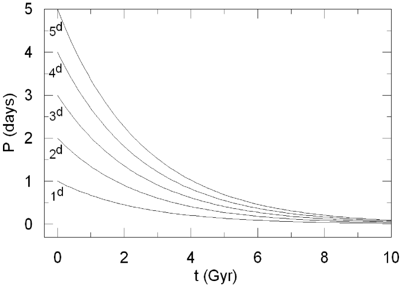
Figure 3: Dynamical evolution of the 62 field CABs for the initial periods from 1 to 5 days.

It is advantageous to have rate coefficients as constants. So, the halving times could be determined as $T_{J}=0.693/\alpha_{J}=1.99\pm 0.36$ Gyr for the OAMs, $T_{P}=0.693/\alpha_{P}=1.75\pm 0.32$ Gyr for the orbital periods and $T_{M}=0.693/\alpha_{M}=5.33\pm 1.16$ Gyr for the systemic masses with a concept similar to half lives of the radioactive elements. Then, $J$, $P$ and $M$ could be expressed by the half times as

$$X=X_{0}~{}e^{-{0.693\over T_{X}}t},$$ (22)

where $X$ could be $J$, $P$ and $M$.

Guinan & Bradstreet (1988) estimated that a detached system with $M=1.10+0.74~{}M_{\odot}$ and initial periods $P_{i}$ = 3.4, 2.3 and 1.2 days, becomes a contact binary with an orbital period $P_{c}$ = 0.315 days at about 4, 1 and 0.7 Gyrs time respectively by the process of AML due to the magnetic braking. However, according to the period decreasing rate derived in this study, a similar system reaches contact configuration of a same contact period at about 6.01, 5.02 and 3.38 Gyrs respectively. Except for the longest period case, the timescale differences are substantial. Such differences are expected since our rate was found statistically and it stands for an average representing all the orbital periods from 0.479 days to several tens of days. Moreover, our rates are lower limits, so our time scale predictions could be only upper limits.

In our estimate we found a system with $M=1.10+0.74~{}M_{\odot}$ would lose 54.2 per cent, 47.9 per cent and 35.6 per cent of its mass in the duration of 6.01, 5.02 and 3.38 Gyrs of pre-contact time. Again, a substantial amount of mass loss seems inevitable. Even if radius change during main-sequence lifetime ($\sim 10$ Gyr for a solar mass star) could be ignored, a better modeling with a nuclear and radius evolution could be prompted if one considers such an amount of mass loss. However, the dynamical evolutions of short-period systems like ER Vul and XY UMa which have components on the main-sequence, could be predicted rather consistently by assuming their present radii stay unchanged.

The present orbital period of ER Vul is $P_{0}$ = 0.698 days. It is a detached system with two main-sequence $(G0V+G5V)$ stars having masses $M=1.10+1.05~{}M_{\odot}$ and radii $R_{1}+R_{2}=1.11+1.08~{}R_{\odot}$.

The semi major axis of ER Vul at the contact configuration can be predicted as $a=a_{1}+a_{2}=2.92~{}R_{\odot}$ by considering that $R_{1}+R_{2}\simeq 0.74a$ in contact configuration (see Kopal 1978). Again, with the present day systemic mass $M=2.15~{}M_{\odot}$ and $a=2.92~{}R_{\odot}$, Kepler’s third law would imply $P_{C}$ = 0.394 days for the contact orbital period. Then, using the 1.75 Gyr of halving time for orbital period, eq. (22) predicts 1.44 Gyr for ER Vul to reach the contact configuration.

However, $\Delta T$ = 1.44 Gyr of time duration causes ER Vul to lose 17.1 per cent of its mass. Since this mass loss has not been considered in the first order estimation of the $P_{C}$, the $P_{C}$ must be under and $\Delta T$ must be over estimated. After only five steps of iterations, $P_{C}$ = 0.427 days and 14.9 per cent mass loss becomes consistent with $\Delta T$ = 1.238 Gyr for ER Vul to reach a contact configuration. At least we could claim this is the upper limit according to the empirical estimate of the decreasing rates of $J$, $P$ and $M$ from the kinematics of CABs.

4 conclusions

The well known spin-down of single stars due to AML requires orbital shrinkage (period decrease) in close binary systems. For this process to be effective, the spin-orbit coupling $(P_{s}\cong P_{orb})$ consequence of tidal locking was already suggested to be a necessary condition (Guinan & Bradstreet 1988; van’t Veer & Maceroni 1988, 1989; Stepien 1995). Thus, long period binaries with no tidal locking are not expected to evolve into shorter period systems since tidal locking would be ineffective in transferring orbital angular momentum to the spinning components where magnetic braking operates.

With a shrinking orbit, the more massive component of a short period binary may fill its Roche lobe faster and start transferring mass to the other component, while the system is still evolving towards shorter periods under the wind-driven mass loss and spin-orbit coupling mechanism. Only after Roche lobe overflow starts, AM evolution of the binary becomes dominated by the mass transfer. Until the mass-ratio reversal, the orbital period should be decreasing. But during the second stage, after the mass ratio reversal, the orbital period is expected to increase, that is, opposite to shrinking, and the orbit starts to enlarge.

The sample of this study contains detached CABs with orbital period greater than 0.479 days (XY UMa). A direct period limit to tidal locking is not known. However, to obtain undistorted statistical results, lower limits are applied (2.4 days by van’t Veer & Maceroni 1988, and 10 days by Demircan 1999). This limit appears to be the function of the total mass, the orbital period, as well as age of the system (see, Tassoul 2000). By comparing orbital and rotation periods in Table 1 and Table 2, we estimated that it is not less then about $\sim 70$ days in the field CABs and around 10 days in the MG CABs. However, the MG CABs are not fully effective to give age dependent variations in $J$, $M$ and $P$ and there are only two systems with $P>70$ days in the field CABs (see Table 2). Thus, we just ignored the tidal locking limit to the orbital period of field CABs.

Nevertheless, the tidal or the magnetic locking, in principle, does not involve a mass loss directly. But, it is a mechanism which transfers OAM to the components, where the AM is lost by magnetically driven stellar winds. The magnetic field lines, especially the ones which are perpendicular to the stars surface and could reach up to the Alfven radius, enforces plasma to co-rotate. As long as the mass is lost from the Alfven radius, not from the surface directly as in the case of isotropic winds, angular momentum loss per particle appears to be amplified. Since OAM loss becomes associated with the mass loss and there is a mechanism which amplifies angular momentum loss per particle, the condition derived from eq. (12) will be valid.

The amplification factor could differ from one system to another. However the general trend, as implied by the plots in Fig. 2, indicates that the average amplification ($\bar{A}$) must be bigger than 5/3 for the majority (perhaps all) of CABs so that the decrease of $P$ together with the decrease of $J$ and $M$ by age is observed. Otherwise, if $\bar{A}<5/3$, the orbital periods would have increased despite the mass and OAM loss. The average amplification factor for the present sample could be determined as

$${\bar{A}}={{dJ\over dt}{1\over J}\over{dM\over dt}{1\over M}}={{\alpha_{J}\over\alpha_{M}}=2.68}.$$ (23)

If such an amplification mechanism operates among the CABs, one must expect the rate coefficients $\alpha_{J}$, $\alpha_{M}$ and $\alpha_{P}$ must hold a relation

$$3{\alpha_{J}}=5{\alpha_{M}}+{\alpha_{P}}$$ (24)

according to eq. (6). Replacing $\alpha_{J}$ by $\bar{A}\alpha_{M}$ according to eq. (23), eq. (24) reduces to

$${(3\bar{A}-5)}{\alpha_{M}}={\alpha_{P}},$$ (25)

which implies that the decreasing rate of orbital periods can also be predicted from the amplification parameter and the mass loss rate if they are known.

The mean amplification factor $\bar{A}$ = 2.68, and the mean mass loss rate $\alpha_{M}=1.30\times 10^{-10}yr^{-1}$ for the present sample of CABs require the mean rate of orbital period decrease to be $3.95\times 10^{-10}yr^{-1}$ according to above relation. It is indeed interesting that this computed value agrees with the value $3.96\times 10^{-10}yr^{-1}$ which was found independently from the regression analysis of linear line fitting to $P$ data in Table 3. So we can conclude that the present data confirm the orbital period decrease as a cause of the mass loss from CAB systems with a mechanism which is sufficient to draw 2.68 times more OAM than isotropic mass loss from the component surfaces.

As for the direct confirmation of the predicted continuous orbital period decreases by O–C diagrams, it is known in general that the changes as small as about $10^{-9}$ days in systems with periods around one day would be observable over a timespan of a century. However, in the case of CABs, because of the large scatter and fluctuations due to magnetic activity or due to third body with light-time effect in the O–C diagrams, it may not possible to detect our prediction of continuous orbital period decreases which operate in a much larger time-scale which is comparable to main-sequence evolutionary times.

5 Acknowledgments

We would like to thank Edwin Budding and anonymous referee for their useful comments.

References

- [1] Abt H.A., Levy S.G., 1976, ApJS, 30, 273
- [2] Abt H.A., 1983, ARA&A, 21, 343
- [3] de Medeiros J.R., Udry S., 1999, A&A, 346, 532
- [4] Demircan O., 1999, Tr. J. Phys., 23, 425
- [5] Demircan O., 2000, in Variable Stars as Essential Astrophysical Tools, ed. C İbanoğlu. Dordrecht; Boston (NATO Science Series. Series C. Mathematical and Physical Sciences; Vol 544), p.615
- [6] Demircan O., 2002, in The Royal Road to Stars, ed. O Demircan, E Budding. Publications of COMU, Çanakkale, Turkey, p.130
- [7] Eaton J.A., Barden S.C., 1988, AcA, 38, 353
- [8] Eggen O.J., 1958a, MNRAS, 118, 65
- [9] Eggen O.J., 1958b, MNRAS, 118, 154
- [10] Eggen O.J., 1989, PASP, 101, 366
- [11] Eggen O.J., 1995, AJ, 110, 2862
- [12] Eker Z., 1987, MNRAS, 228, 869
- [13] Farinella P., Luzny F., Mantegazza L., Paolicchi P., 1979, ApJ, 234, 973
- [14] Ghez A.M., Neugebauer G., Matthews K., 1993, AJ, 106, 2005
- [15] Huang S.S., 1966, ARA&A, 4, 35
- [16] Huenemoerder D.P., Barden, S.C., 1986, AJ, 91, 583
- [17] Guinan E.F., Bradstreet D.H., 1988, in Dupree A.K., Lago M.T., eds, Formation and Evolution of Low Mass Stars, Kluwer, Dordrecht, p. 345
- [18] Karataş Y., Bilir S., Eker Z., Demircan O., 2004, MNRAS, 349, 1069
- [19] Kraft R.P., 1967, ApJ, 150, 551
- [20] Kreiner J.M., Kim C., Nha, II-Seung, 2001, on Atlas of O–C Diagrams of Eclipsing binary Stars, Poland: Wydawnictwo Noukowe Akademii Pedagagicznej
- [21] Kopal Z., 1978, in Z. Kopal, eds, Dynamics of Close Binary Systems, Dordrecht Reidel Publ. Co., p. 332
- [22] Maceroni C., van’t Veer F., 1991, A&A, 246, 91
- [23] Mestel L., 1968, MNRAS, 138, 359
- [24] Mestel L., 1984, in S.L. Baliunas and L. Hartmann, eds, the Third Cambridge Workshop Cool Stars, Stellar Systems, and the Sun, Lecture Notes in Physics, Vol. 193, Springer-Verlag, Berlin, Heidelberg, New York, p. 49
- [25] Montes D., Lopez-Santiago J., Galvez M.C., Fernandez-Figueroa M.J., De Castro E., Cornide M., 2001a, MNRAS, 328, 45
- [26] Montes D., Fernandez-Figueroa M.J., De Castro E., Cornide M., Latorre A., 2001b, in J. Garcia Lopez, R. Rebolo, & M.R. Zapaterio, eds, ASP Conf. Ser. Vol. 223, 11th Cambridge Workshop on Cool Stars, Stellar Systems and the Sun, Astron. Soc. Pac., San Francisco, p. 1477
- [27] Okamoto I., Sato K., 1970, PASJ, 22, 317
- [28] Olson E.C., 1989, AJ, 98, 1002
- [29] Popper D.M., 1991, AJ, 101, 220
- [30] Pringle J.E., 1985, in Pringle J.E., Wade R.A., eds, Interacting binary stars, Cambridge University Press, Cambridge, p. 1
- [31] Schatzman E., 1959, A&AS, 8, 129
- [32] Skumanich A., 1972, ApJ, 171, 565
- [33] Stepien K., 1995, MNRAS, 274, 1019
- [34] Strassmeier K.G., Hall D.S., Zeilik M., Nelson E., Eker Z., Fekel F.C., 1988, A&AS, 72, 291
- [35] Strassmeier K.G., Hall D.S., Fekel F.C., Scheck M., 1993, A&AS, 100, 173
- [36] Tassoul, J.L., 2000, in Stellar Rotation, Cambridge; New York, Cambridge Univ. Press, p.18
- [37] van’t Veer F., 1979, A&A, 80, 287
- [38] van’t Veer F., Maceroni C., 1988, A&A, 199, 183
- [39] van’t Veer F., Maceroni C., 1989, A&A, 220, 128
- [40] Vilhu O., Rahunen T., 1980, in Plavec M.J., Popper D.M., Ulrich D.R., eds, Proc. IAU Symp. 88, Close Binary stars, Reidel, Dordrecht, p. 491
- [41] Wielen R., 1982, Numerical data and Functional Relationships in Science and Technolgy. Springer-Verlag, Berlin, p. 29
- [42] Williamon R.M., Van Hamme W., Torres G.T., Sowell J.R., Ponce V.C., 2005, AJ, 129, 2798