Gradient and dispersion analyses of the WMAP data

Abstract

We studied the WMAP temperature anisotropy data using two different methods. The derived signal gradient maps show regions with low mean gradients in structures near the ecliptic poles and higher gradient values in the wide ecliptic equatorial zone, being the result of non-uniform observational time sky coverage. We show that the distinct observational time pattern present in the raw (cleaned) data leaves also its imprints on the composite CMB maps. Next, studying distribution of the signal dispersion we show that the north-south asymmetry of the WMAP signal diminishes with galactic altitude, confirming the earlier conclusions that it possibly reveals galactic foreground effects. As based on these results, one can suspect that the instrumental noise sky distribution and non-removed foregrounds can have affected some of the analyses of the CMB signal. We show that actually the different characteristic axes of the CMB sky distribution derived by numerous authors are preferentially oriented towards some distinguished regions on the sky, defined by the observational time pattern and the galactic plane orientation.

1 Introduction

The first-year data from the Wilkinson Microwave Anisotropy Probe (WMAP) (Bennett at al. 2003a,b) became a basis for testing cosmological scenarios, substantial improving of evaluation accuracy of basic cosmological parameters related to the geometry of our Universe, dynamics of its expansion, matter and energy contents. Therefore any studies of reliability of the provided data are of great interest and importance. In particular, application of non-standard methods provide additional independent tests of data quality and consistency, as well as the correctness of involved interpretations.

All the sky CMB anisotropy maps give possibility to test with high accuracy the fundamental principles of current cosmology, such as the isotropy of our Universe and the Gaussianity of primordial cosmological perturbations. The first analysis of WMAP data for Gaussianity was performed by WMAP team Komatsu et al. (2003). They found that the WMAP data are consistent with the Gaussian primordial fluctuations and provided limits to the amplitude of non-Gaussian ones. Other authors, however, applying advanced or sophisticated statistical methods to analyse the foreground-subtracted WMAP maps pointed out non-Gaussian signatures or north-south asymmetry of galactic hemispheres (Chiang et al. 2003, Park 2004, Eriksen et al. 2004a, Hansen et al. 2004a,b,c, Eriksen et al. 2005a, Cayon et al. 2005). Some authors suppose that it may be caused by residual foreground contamination from unknown galactic or extra-galactic sources and find their possible locations, angular scales, and amplitudes (Park 2004, Eriksen et al. 2004a, Hansen et al. 2004b, Chiang & Naselsky 2004, Patanchon et al. 2004, Naselsky et al. 2005, Tojeiro et al. 2005, Land & Magueijo 2005). For example, Tojeiro et al. (2005) argued that the evidence for non-Gaussianity on large scales is associated with cold spots of unsubtracted foregrounds. Some part of non-Gaussian statistics of $\Delta T/T$ fluctuations can be due to the ring of pixels of radius of 5 degrees centered at ($l\approx 209^{o},b\approx-57^{o}$) Cayón et al. (2005), close to the spot detected in Vielva et al. (2004) and Cruz et al. (2005). Wibig & Wolfendale (2005) performed the correlation analysis of CMB temperature and gamma-ray whole-sky maps and detected positive correlation, which may suggest an actual contamination of the WMAP data by, if not cosmic rays directly, some component accompanying them in interstellar space with a sufficiently flat emission spectrum.

All these studies indicate that WMAP Q-, V-, and W-band maps contain information on unidentified extended low-amplitude foreground structures that contaminate the relic CMB signal. The effective extraction of these structures from the WMAP maps would improve the current and future CMB analyses, as well as reveal possible new foreground objects or effects (cf. Davies et al. 2005, Eriksen et al. 2005b).

Our principal goal in the present paper is to understand the physical meaning of structures within WMAP measurements in order to detect or limit possible non-cosmological factors affecting the data used for determining cosmological parameters. We apply two simple analytical methods to study possible foreground or observational effects in the WMAP first-year data, not recognized and/or p removed by the cleaning methods used by the WMAP team (Bennett et al. 2003b). In the paper, first we shortly provide the basic information about the data analysed, and next describe our method of generating gradient maps from the foreground-cleaned WMAP maps and interpret the large-scale gradient structures by the observational strategy of the WMAP satellite. We demonstrate that the scanning effects present in the raw signal data can leave clear imprints on the gradients maps from all frequency channels, retained even in coadded, smoothed, and ILC maps. Then, we investigate distribution of signal dispersion in the WMAP maps to find a significant asymmetry between the northern and southern galactic hemispheres. Following some previous authors, we argue that a natural explanation of this asymmetry is residual galactic contamination. Finally, the inevitable influence of the above-mentioned effects on the analysis of the large-scale CMB structure is shortly considered.

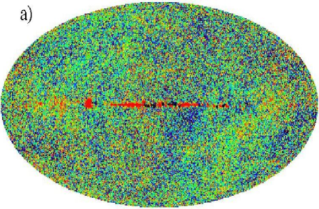
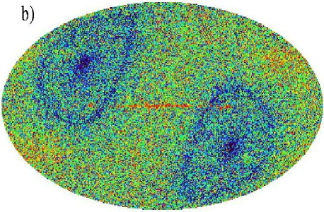
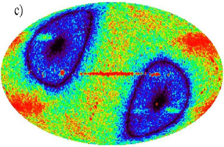
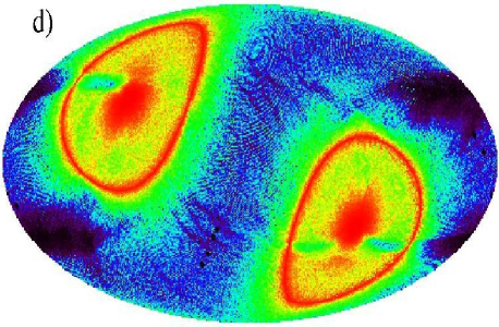
Figure 1: The maps in the Mollveide projection of the galactic coordinate frame present: a) the signal $\Delta T$ in the WMAP V2 channel; b) the V2 gradient map derived from (a), blue color denotes low gradient values and red color - higher ones; c) the V2 gradient map smoothed out using the $1\degr\,$ Gaussian beam; d) the effective number of observation map for the channel V2; blue color denotes small numbers and red color - larger ones. All maps are presented in the histogram-scale format to enhance the apparent features. The structures in the galactic plane have roughly about ten times higher gradients than those outside it.

2 The observational data

In this paper we study the publicly available first-year WMAP maps in 5 frequency channels, K (22.8 GHz), Ka (33.0 GHz), Q (40.7 GHz), V (60.8 GHz) and W (93.5 GHz) downloaded from LAMBDA website. The maps provide distributions of differential temperature measured in micro-Kelvin units, $\Delta T$, over the entire sky. The signal in each individual map, after subtracting the kinematic dipole component, foreground point sources, and diffuse galactic emission, is expected to consist primarily of cosmic microwave background (see Bennett et al. 2003a,b for details). We studied mainly individual differential assemblies maps with the full available resolution (NSIDE=512 in the HEALPix pixelization). Most analyses presented in the paper use the V2 channel map, showing the lowest galactic contamination and small instrumental noise.

3 Gradient analysis of the WMAP CMB anisotropy maps

3.1 Derivation of gradient maps

We study the variations of measured temperature fluctuations in the WMAP sky maps, including CMB signal and instrumental noise, by analysing the gradient structure of the data. We applied two methods in order to derive the gradients. In the first approach, we evaluate the maximum gradient value at a given location in the map (i.e. in each pixel/cell) calculated between the reference cell and the surrounding cells using:

$$({\rm grad}\,\Delta T)_{0,max}=Max\left|{\Delta T_{i}-\Delta T_{0}\over d_{i,0}}\right|\qquad,$$

where the index ”$0$” indicates the reference cell. ”$i$” runs through all adjacent cells and $d_{i,0}$ is the distance between the cells considered . The second approach involved deriving a gradient map with the use of the Sobol operator (filter) known in the image analysis as the edge detector (Huang et al. 2003). This method evaluated the mean gradient at a given pixel using the relative values of the signal, $\Delta T_{i}$, in its 8 adjacent pixels. In this case, the obtained gradient maps reveal the same pattern as in the maximum gradient method, but the derived mean gradient values are lower. Below we present the maximum gradient maps derived with the simpler method using eq. (3.1), which is more efficient in visualizing gradient structures.

The map of $({\rm grad}\,\Delta T)_{0,max}$ derived for the WMAP V2 channel is presented in Fig. 1b. In the figure one can clearly see regions of low gradients at both the ecliptic poles and within two extended circular regions around the poles at the radius $\approx 23^{\circ}$. The extended regions of enhanced gradient occupy a wide stripe along the ecliptic equator. The largest gradients occur at the galactic plane due to some residual galactic component. Relatively large gradient values are also found in places where data were partly discarded because of the planets appearing in the WMAP field of view. The comparison of the gradient pattern with the map of observational time ($\equiv$ the effective number of observations in the WMAP team nomenclature, $N$) (Fig.1d) proves that most of the observed extended gradient structures represent variations of instrumental noise within the data. The noise distribution corresponds to the varying observational time in different areas of the sky due to the WMAP sky scanning pattern. It also leads to a distinct anti-correlation between the observational time and the signal gradient.

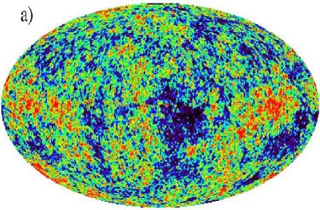
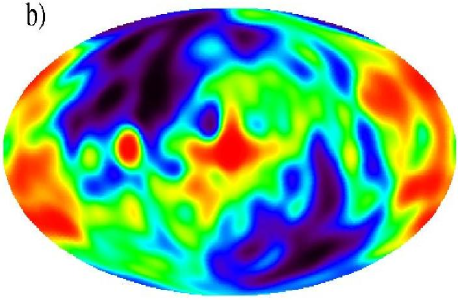
Figure 2: a) An ILC map of the CMB temperature fluctuations and b) its gradient map smoothed with the $15\degr\,$ Gaussian beam.

3.2 Analysis of gradient pattern

Using the above method, we derived the gradient maps for all the WMAP channels (the maps can be obtained upon request from K.Ch.) with analogous characteristic gradient patterns, spots at galactic poles, and rings around them. These characteristic features in the gradient distribution are more distinct after smoothing the maps (Fig. 1c). In order to show it quantitatively, we smoothed both the V2 CMB and the number of observation maps with increasing Gaussian beams, and calculated the correlation coefficient. Without smoothing, the correlation is -0.16, for 1° smoothing it is -0.26, and for 5°, 10°, and 15° smoothing it becomes -0.69, -0.83, and -0.89, respectively.

We also obtained the gradient maps from the coadded maps for individual assemblies in V, Q and W bands, with the position-dependent, or band-dependent inverse noise-weighting. We got gradient patterns much similar to those obtained from the V2 channel alone. Next we applied the gradient analysis to the ILC map. In this case, the characteristic gradient pattern is weaker, because of the convolved to 1° scale component maps of the ILC combined map. However, the distinct pattern appears also in this case, as we demonstrate at Fig. 2b by convolving the gradient map with the 15° Gaussian beam. In the figure, the observational time pattern analogous to that in Fig. 1d is clearly reproduced, while significantly perturbed by the effects of CMB or galactic foreground signal structures.

The performed experiments confirm that the systematic pattern revealed in the gradient maps is firmly established and cannot be removed by simple filtering procedures, like convolving, or adding data maps. Thus it can affect the analysis and interpretation of the large-scale distribution of the signal in the WMAP maps.

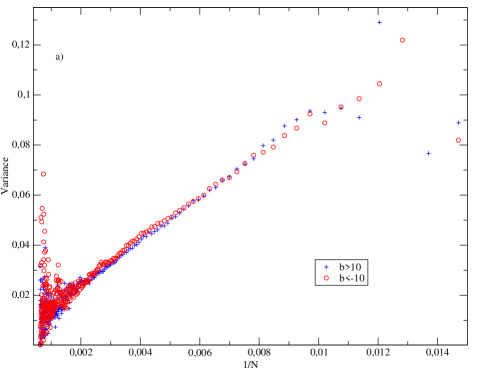
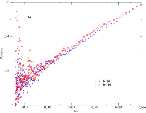
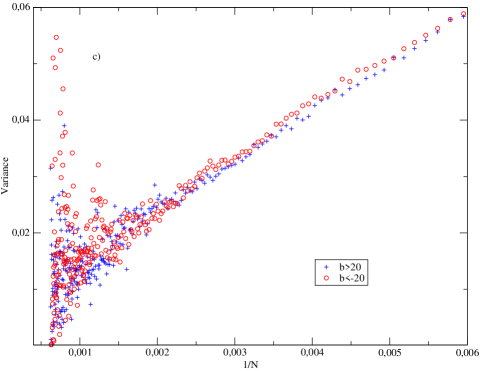
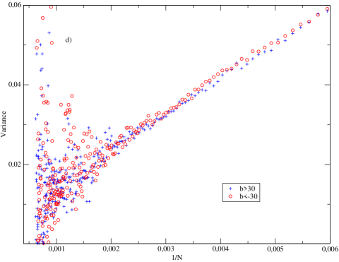
Figure 3: Values of the measured variance $\sigma^{2}$ versus the number of observations $1/N$ for the V2 sky map.

4 Asymmetric noise distributions of galactic hemispheres

Apart from the above analysis of signal gradients, we studied also the large-scale asymmetries within the WMAP data by deriving diagrams of the measured signal variance across the sky versus the effective number of observations, N. Such diagrams, presented by Jarosik et al. (2003) for the whole sky (see their Fig.10), we constructed independently for the northern and southern galactic hemispheres, in a couple of galactic polar-cap regions formed by removing the galactic equatorial strip with $|b|<10^{\circ}$, $20^{\circ}$ and $30^{\circ}$ (Fig. 3). We used these growing galactic cuts to check if possible galactic foregrounds may affect the data. To derive the sample signal variance for a consecutive bin ”$i$” centered at the number of observations $N_{i}$ we used data from all strip cells with $N$ in the respective range ($N_{i}-2.5$, $N_{i}+2.5$). There were also much smaller numbers of cells with very small or very large $N$, which can explain growing scatter at limiting parts of the plot presented in the upper-left panel of Fig 3. In the other three panels in this figure the zoomed distributions are presented, excluding the range with low $N$, where the linear form of distribution is lost. In the figure one can easily see the south-north asymmetry in the variance distribution. The difference is preserved in a range of regions in the sky with varying number of observations. Moreover, there is a distinct tendency for decreasing the difference between hemispheres at higher galactic latitudes.

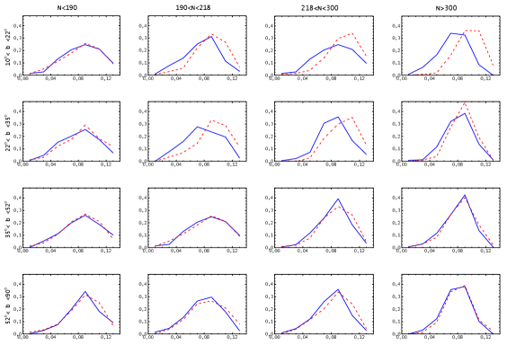
Figure 4: Histogram points connected with lines showing the signal dispersion $\sigma_{signal}\equiv\sqrt{<\Delta T_{signal}^{2}>}$ distributions at 4 different galactic altitude stripes ($b\in$ [$10^{\circ}$, $22^{\circ}$] - first row, [$22^{\circ}$ , $35^{\circ}$] - second row, [$35^{\circ}$, $52^{\circ}$] - third row, and the polar cup [$52^{\circ}$, $90^{\circ}$] - forth row) in different observational time intervals (N¡190), 190¡N¡218, 218¡N¡300, N¿300). The measured dispersion is presented along the horizontal axis of each panel in 0.02 bins. In the following panels the results are compared for the northern galactic hemisphere (full line) and for the southern one (dashed line).

We performed another analysis of the signal dispersion in the channel V2. We considered 4 separate galactic altitude stripes ($b\in$ [$10$, $22$], [$22$, $35$], [$35$, $52$], [$52$, $90$]) and 4 ranges of the observational time ($N<190$, $190<N<218$, $218<N<300$, $N>300$), separately in both hemispheres. The individual dispersion values were derived in the following way. We assumed a strict relation to hold between dispersions of the cosmic signal (dominated by the CMB) fluctuations, $\sigma_{cs}$, and of the instrumental noise, $\sigma_{noise}(N)=\sigma_{0}/\sqrt{N}$, constituting the measured dispersion $\sigma$ of temperature fluctuations ($\Delta T$) on the map,

$$\sigma^{2}=\sigma_{\rm cs}^{2}+{\sigma_{0}^{2}\over N}\qquad.$$

The noise constant for the analysed V2 channel is given by the WMAP team as $\sigma_{0}=2.93683$ (Bennett et al. 2003a). Our operational procedure to derive the individual dispersion value involves data from n ($\approx 300$) consecutive cells from the V2 sky map (for the given stripe and the observation number range):

$$\sigma_{\rm cs}=\sqrt{{\left[\sum_{i=1}^{n}(\Delta T_{i})^{2}\right]\over n}-{\sigma_{0}^{2}\over N}}\qquad.$$

One may note that the presented algorithm, while not supposed to yield strict statistical quantities, provides a uniform measure of fluctuation amplitude, allowing for comparing the sky signal in both hemispheres.

The normalized distributions of the above dispersion values $\sigma_{\rm cs}$ are presented at Fig. 4. A distinct systematic trend can be observed in the successive panels, with the south-hemisphere distributions shifted to higher dispersion values. The observed difference is larger in sky stripes closer to the galactic plane and within these stripes is more pronounced for panels with larger $N$ (the longer observational times). However, in regions near the galactic poles such weak but regular shift is also observed.

5 Summary and Conclusions

The gradient analysis is a very efficient method in recognition of weak signal non-uniformities in the sky maps. By analysing the gradient maps we demonstrate the WMAP noise pattern resulting from non-uniformity of the observational time distribution. The pattern involves regions of low noise (small gradients) near the ecliptic poles and along the circles at the angular distance of $\approx 23^{\circ}$ from the ecliptic poles, and non-uniform extended regions of larger noise amplitudes (larger gradients) along the ecliptic equator. The pattern introduced by local variations in the observational time is much alike at all available frequency channels and must inevitably affect the resulting CMB maps, independently of the applied approach to constructing such maps from the original data (e.g. Bennett at al. 2003b, Eriksen et al. 2004b, Tegmark et al. 2003). The apparent gradient structure can ”propagate” through the noise filtering procedures used in attempt to reconstruct the CMB signal maps, as it is proved in section 3 by showing its imprints in the frequently presented and discussed ILC map. It suggests that analyses of the ILC maps, or similar maps, must be affected - besides statistical flaws due to the signal generation procedure and non-removed foreground effects - by the WMAP observational time pattern (cf. in this context e.g. Fig. 1 in Hansen et al. 2004c, Fig. 4 in Jaffe et al. 2005a and Jaffe et al. 2005b). One may also note that for the CMB study based on the WMAP data (and the future Planck mission) the best regions to study are those with the lowest gradients around the ecliptic poles, and the lowest instrumental noise.

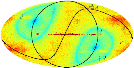
Figure 5: The V2 gradient map from Fig. 1c (but in a linear scale) with plotted characteristic directions described in the text. For orientation, the lines are added for the ecliptic equator and the ecliptic meridian perpendicular to the galactic plane.

Independently, the possible galactic foreground effects were studied by simple methods of analysing distributions of signal fluctuations versus the observational time at the WMAP V2 band. We confirm existence of the south-north asymmetry between hemispheres, with the larger fluctuation amplitude in the south hemisphere (cf. Eriksen et al. 2004a, Hansen et al. 2004a,b). We show that the asymmetry extends throughout a large part of the sky and diminishes at higher galactic altitudes. It suggests that the foreground effects may be due to some galactic component concentrating along the galactic plane. Furthermore, higher amplitude of signal fluctuations in the southern hemisphere can be, in our opinion, explained by the known fact that our Sun is situated approximately 20 pc north off this plane. Let us also note that regularity of observed effects with growing galactic altitude, also in the separate ranges of $N$ at Fig. 4, does not support the hypothesis suggesting an extragalactic origin of the asymmetry.

The findings suggest that the analysis of large-scale patterns of the CMB signal based on the WMAP data must be affected by observational time non-uniformities, which are not possible to be quite removed. Thus we expect that analysis results of the global CMB sky distribution can be also influenced by this fact, introducing the ecliptic symmetry to the data, and by the foreground effects, leading to some symmetry/asymmetry with respect to the galactic plane. Thus let us look at examples of characteristic orientations/axes of the universal CMB distribution discovered by the other authors (e.g. in discussion of non-trivial universe topology by de Oliveira-Costa et al. 2004, Weeks et al. 2004, Roukema et al. 2004). Such 10 directions imposed onto the gradient map in Fig. 5 include: 1.) ($l=207^{\circ}$, $b=-59^{\circ}$) Vielva et al. (2004); 2) (222^∘, -62^∘) Jaffe et al. (2005a); 3) (-100^∘, 60^∘) Land et al. (2005); 4) (-110^∘, 60^∘) de Oliveira et al. (2004); 5) (252^∘ , 65^∘); 6) (51^∘, 51^∘); 7) (144^∘, 38^∘); 8) (271^∘, 3^∘); 9) (207^∘, 10^∘); 10) (332^∘, 25^∘) Roukema et al. (2005). The presented directions show more or less preferential orientation with respect to four circles: the ecliptic equator and its meridian perpendicular to the galactic plane, plus two small circles in the distance of $23^{\circ}$ around the ecliptic poles, the sites corresponding to the local maxima of the observational time distribution. Also the discussed unexplained quadrupole and octopole orientations in respect to the ecliptic frame (cf. de Oliveira-Costa et al. 2004, Land & Magueijo 2005, Jaffe et al. 2005) can be possibly explained in a natural way, if their detections are affected by the sky pattern due to the observational time, retained in the cleaned maps.

In the present work we were not able to verify the supposition that several detected structures in the CMB maps result from the discussed instrumental or foreground effects, but the distinct grouping of the observed structure orientations within some regions of the ecliptic and galactic reference frames suggests that such possible effects should be properly considered.

This work made use of the WMAP data archive and the HEALPIX software package. We are grateful to Reinhard Schlickeiser and Andrzej Woszczyna for stimulating discussions. The work was performed within the research program of the Jagiellonian Center of Astrophysics.

References

- (1) Bennett C.L., Halpern M., Hinshaw G. et al., 2003a, ApJS, 148, 1
- (2) Bennett C.L., Hi;; R.S., Hinshaw G. et al., 2003b, ApJS, 148, 97
- Cayón et al. (2005) Cayón L., Jin J., Treaster A., 2005, MNRAS, 362, 826
- Chiang et al. (2003) Chiang L.-Y., Naselsky P.D., Verkhodanov O.V., Way M.J., 2003, ApJ, 590, L65
- Chiang & Naselsky (2004) Chiang L.-Y., Naselsky P.D., 2004, astro-ph/0407395
- Cornish et al. (2004) Cornish N.J., Spergel D.N., Starkman G.D., Komatsu E., 2004, Phys. Rev. Lett., 92, 201302
- Cruz et al. (2005) Cruz M., Martinez-Gonzalez E., Vielva P., Cayon L. 2005, 356, 29
- de Oliveira-Costa et al. (2004) de Oliveira-Costa A., et al., 2004, Phys. Rev. D, 69, 063516
- Davies et al. (2005) Davies R.D., Dickinson C., Banday A.J., Jaffe T.R., Górski K.M., 2005, astro-ph/0511384
- (10) Eriksen H.K., Hansen F.K., Banday A.J., Górski K.M., Lilje, P.B., 2004a, ApJ, 605, 14
- (11) Eriksen H.K., Banday A.J., Górski and Lilje, P.B., 2004b, ApJ, 612, 633
- (12) Eriksen H.K., Banday A.J., Górski and Lilje, P.B., 2005a, ApJ, 622, 58
- (13) Eriksen, H. K. et al., 2005b, astro-ph/0508268
- (14) Hansen F.K., Banday A.J, Górski K.M., 2004a, MNRAS, 354, 641
- (15) Hansen F.K., Balbi A., Banday A.J, Górski K.M., 2004b, MNRAS, 354, 905
- (16) Hansen F.K., Cabella P., Marinucci D., Vittorio N., 2004c, ApJ, 607, L67
- (17) Huang L.-L., Shimizu A., Hagihara Y., Kobatake H., 2003, Pattern Recogniction 36, 2501
- (18) Jaffe T.R., Banday A.J., Eriksen H.K., Górski K.M., Hansen F.K., 2005a, ApJ, 629, L1
- (19) Jaffe T.R., Banday A.J., Górski K.M., Lilje P.B., 2005b, astro-ph/0508196
- Jarosik et al. (2003) Jarosik N., Barnes C., Bennett C.L. et al., 2003, ApJS, 148, 29
- Komatsu et al. (2003) Komatsu E., Kogut A., Nolta M.R. et al., 2003, ApJS, 148, 119
- Land & Magueijo (2005) Land K., Magueijo J., 2005, MNRAS 362, L16
- Naselsky et al. (2005) Naselsky P.D., Novikov I.D., Chiang L.-Y., 2005, astro-ph/0506466
- Patanchon et al. (2004) Patanchon G., Cardoso J.-F., Delabrouille J., Vielva P., 2004, astro-ph/0410280
- Park (2004) Park C.-G., 2004, MNRAS, 349, 313
- Roukema et al. (2004) Roukema B.F., Lew B., Cechowska M., Marecki A., Bajtlik S., 2004, A&A, 423, 821
- Tegmark et al. (2003) Tegmark M., de Oliveira-Costa A., Hamilton A.J.S., 2003, Phys.Rev.D, 68, 123523
- Tojeiro et al. (2005) Tojeiro R., Castro P.G., Heaves A.F., Gupta S., 2005, astro-ph/0507096
- Vielva et al. (2004) Vielva P., Martinez-Gonzalez E,Barreiro R.B., Sanz J.L. & Cayon L. 2004, ApJ, 609,22
- Weeks et al. (2004) Weeks J., Luminet J.-P., Riazuelo A., Lehoucq R., 2004, MNRAS, 352, 258
- Wibig & Wolfendale (2005) Wibig T., Wolfendale A.W., 2005, MNRAS, 360, 236