Dimensionless constants, cosmology and other dark matters

Abstract

We identify 31 dimensionless physical constants required by particle physics and cosmology, and emphasize that both microphysical constraints and selection effects might help elucidate their origin. Axion cosmology provides an instructive example, in which these two kinds of arguments must both be taken into account, and work well together. If a Peccei-Quinn phase transition occurred before or during inflation, then the axion dark matter density will vary from place to place with a probability distribution. By calculating the net dark matter halo formation rate as a function of all four relevant cosmological parameters and assessing other constraints, we find that this probability distribution, computed at stable solar systems, is arguably peaked near the observed dark matter density. If cosmologically relevant WIMP dark matter is discovered, then one naturally expects comparable densities of WIMPs and axions, making it important to follow up with precision measurements to determine whether WIMPs account for all of the dark matter or merely part of it.

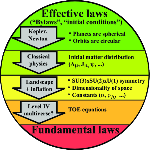
Figure 1: The shifting boundary (horizontal lines) between fundamental laws and environmental laws/effective laws/initial conditions. Whereas Ptolemy and others sought to explain roughly spherical planets and circular orbits as fundamental laws of nature, Kepler and Newton reclassified such properties as initial conditions which we now understand as a combination of dynamical mechanisms and selection effects. Classical physics removed from the fundamental law category also the initial conditions for the electromagnetic field and all other forms of matter and energy (responsible for almost all the complexity we observe), leaving the fundamental laws quite simple. A prospective theory of everything (TOE) incorporating a landscape of solutions populated by inflation reclassifies important aspects of the remaining “laws” as initial conditions. Indeed, those laws can differ from one post-inflationary region to another, and since inflation generically makes each such region enormous, its inhabitants might be fooled into misinterpreting regularities holding within their particular region as Universal (that is, multiversal) laws. Finally, if the Level IV multiverse of all mathematical structures toe exists, then even the “theory of everything” equations that physicists are seeking are merely local bylaws in Rees’ terminology ReesHabitat , that vary across a wider ensemble. Despite such retreats from ab initio explanations of certain phenomena, physics has progressed enormously in explanatory power.

I Introduction

Although the standard models of particle physics and cosmology have proven spectacularly successful, they together require 31 free parameters (Table 1). Why we observe them to have these particular values is an outstanding question in physics.

I.1 Dimensionless numbers in physics

This parameter problem can be viewed as the logical continuation of the age-old reductionist quest for simplicity. Realization that the material world of chemistry and biology is built up from a modest number of elements entailed a dramatic simplification. But the observation of nearly one hundred chemical elements, more isotopes, and countless excited states eroded this simplicity.

The modern $SU(3)\times SU(2)\times U(1)$ standard model of particle physics provides a much more sophisticated reduction. Key properties (spin, electroweak and color charges) of quarks, leptons and gauge bosons appear as labels describing representations of space-time and internal symmetry groups. The remaining complexity is encoded in 26 dimensionless numbers in the Lagrangian (Table 1). All current cosmological observations can be fit with 5 additional parameters, though it is widely anticipated that up to 6 more may be needed to accommodate more refined observations (Table 1).

Table 2 expresses some common quantities in terms of these 31 fundamental ones, with $\sim$ denoting cruder approximations than $\approx$. Many other quantities commonly referred to as parameters or constants (see Table 3 for a sample) are not stable characterizations of properties of the physical world, since they vary markedly with time Scott05 . For instance, the baryon density parameter $\Omega_{b}$, the baryon density $\rho_{b}$, the Hubble parameter $h$ and the cosmic microwave background temperature $T$ all decrease toward zero as the Universe expands and are, de facto, alternative time variables.

Table 1: Input physical parameters. Those for particle physics (the first 26) and $\rho_{\Lambda}$ appear explicitly in the the Lagrangian, whereas the cosmological ones (the last 11) are inserted as initial conditions. The last six are currently optional, but may become required to fit improved measurements. The values are computed from the compilations in PDG ; Mohapatra04 ; inflation .

Parameter	Meaning	Measured value
$g$	Weak coupling constant at $m_{Z}$	$0.6520\pm 0.0001$
$\theta_{W}$	Weinberg angle	$0.48290\pm 0.00005$
$g_{s}$	Strong coupling constant at $m_{Z}$	$1.221\pm 0.022$
$\mu^{2}$	Quadratic Higgs coefficient	$\sim-10^{-33}$
$\lambda$	Quartic Higgs coefficient	$\sim 1$?
$G_{e}$	Electron Yukawa coupling	$2.94\times 10^{-6}$
$G_{\mu}$	Muon Yukawa coupling	$0.000607$
$G_{\tau}$	Tauon Yukawa coupling	$0.0102156233$
$G_{u}$	Up quark Yukawa coupling	$0.000016\pm 0.000007$
$G_{d}$	Down quark Yukawa coupling	$0.00003\pm 0.00002$
$G_{c}$	Charm quark Yukawa coupling	$0.0072\pm 0.0006$
$G_{s}$	Strange quark Yukawa coupling	$0.0006\pm 0.0002$
$G_{t}$	Top quark Yukawa coupling	$1.002\pm 0.029$
$G_{b}$	Bottom quark Yukawa coupling	$0.026\pm 0.003$
$\sin\theta_{12}$	Quark CKM matrix angle	$0.2243\pm 0.0016$
$\sin\theta_{23}$	Quark CKM matrix angle	$0.0413\pm 0.0015$
$\sin\theta_{13}$	Quark CKM matrix angle	$0.0037\pm 0.0005$
$\delta_{13}$	Quark CKM matrix phase	$1.05\pm 0.24$
$\theta_{\rm qcd}$	CP-violating QCD vacuum phase	$<10^{-9}$
$G_{\nu_{e}}$	Electron neutrino Yukawa coupling	$<1.7\times 10^{-11}$
$G_{\nu_{\mu}}$	Muon neutrino Yukawa coupling	$<1.1\times 10^{-6}$
$G_{\nu_{\tau}}$	Tau neutrino Yukawa coupling	$<0.10$
$\sin\theta_{12}^{\prime}$	Neutrino MNS matrix angle	$0.55\pm 0.06$
$\sin 2\theta_{23}^{\prime}$	Neutrino MNS matrix angle	$\geq 0.94$
$\sin\theta_{13}^{\prime}$	Neutrino MNS matrix angle	$\leq 0.22$
$\delta_{13}^{\prime}$	Neutrino MNS matrix phase	$?$
$\rho_{\Lambda}$	Dark energy density	$(1.25\pm 0.25)\times 10^{-123}$
$\xi_{\rm b}$	Baryon mass per photon $\rho_{\rm b}/\ng$	$(0.50\pm 0.03)\times 10^{-28}$
$\xi_{\rm c}$	Cold dark matter mass per photon $\rho_{\rm c}/\ng$	$(2.5\pm 0.2)\times 10^{-28}$
$\xi_{\nu}$	Neutrino mass per photon $\rho_{\nu}/\ng={3\over 11}\sum m_{\nu_{i}}$	$<0.9\times 10^{-28}$
$Q$	Scalar fluctuation amplitude $\delta_{H}$ on horizon	$(2.0\pm 0.2)\times 10^{-5}$
${n_{\rm s}}$	Scalar spectral index	$0.98\pm 0.02$
$\alpha_{n}$	Running of spectral index $d{n_{\rm s}}/d\ln k$	$|\alpha|\mathrel{\hbox to0.0pt{\lower 3.0pt\hbox{$\mathchar 536\relax$}\hss}\raise 2.0pt\hbox{$\mathchar 316\relax$}}0.01$
$r$	Tensor-to-scalar ratio $(Q_{t}/Q)^{2}$	$\mathrel{\hbox to0.0pt{\lower 3.0pt\hbox{$\mathchar 536\relax$}\hss}\raise 2.0pt\hbox{$\mathchar 316\relax$}}0.36$
${n_{\rm t}}$	Tensor spectral index	Unconstrained
$w$	Dark energy equation of state	$-1\pm 0.1$
$\kappa$	Dimensionless spatial curvature $k/a^{2}T^{2}$ Q	$|\kappa|\mathrel{\hbox to0.0pt{\lower 3.0pt\hbox{$\mathchar 536\relax$}\hss}\raise 2.0pt\hbox{$\mathchar 316\relax$}}10^{-60}$

Table 2: Derived physical parameters, in extended Planck units $c=\hbar=G=k_{b}=|q_{e}|=1$.

Parameter	Meaning	Definition	Measured value
$e$	Electromagnetic coupling constant at $m_{Z}$	$g\sin\theta_{W}$	$\approx 0.313429\pm 0.000022$
$\alpha(m_{z})$	Electromagnetic interaction strength at $m_{Z}$	$e^{2}/4\pi=g^{2}\sin^{2}\theta_{W}/4\pi$	$\approx 1/(127.918\pm 0.018)$
$\alpha_{w}$	Weak interaction strength at $m_{Z}$	$g^{2}/4\pi$	$\approx 0.03383\pm 0.00001$
$\alpha_{s}$	Strong interaction strength at $m_{Z}$	$g_{s}^{2}/4\pi$	$\approx 0.1186\pm 0.0042$
$\alpha_{g}$	Gravitational coupling constant	$Gm_{\rm p}^{2}/\hbar c=m_{\rm p}^{2}$	$\approx 5.9046\times 10^{-39}$
$\alpha$	Electromagnetic interaction strength at $0$	$\sim\left[\alpha(m_{z})^{-1}+{2\over 9\pi}\ln{m_{z}^{20}\over m_{u}^{4}m_{c}^{4}m_{d}m_{s}m_{b}m_{e}^{3}m_{\mu}^{3}m_{\tau}^{3}}\right]^{-1}$	$1/137.03599911(46)$
$m_{W}$	$W^{\pm}$ mass	$vg/2$	$(80.425\pm 0.038)\>{\rm GeV}$
$m_{Z}$	$Z$ mass	$vg/2\cos\theta_{W}$	$(91.1876\pm 0.0021)\>{\rm GeV}$
$G_{F}$	Fermi constant	$1/\sqrt{2}v^{2}$	$\approx 1.17\times 10^{-5}\>{\rm GeV}^{-2}$
$m_{H}$	Higgs mass	$\sqrt{-\mu^{2}/2}$	100-250 GeV?
$v$	Higgs vacuum expectation value	$\sqrt{-\mu^{2}/\lambda}$	$(246.7\pm 0.2)\>{\rm GeV}$
$m_{e}$	Electron mass	$vG_{e}/\sqrt{2}$	$(510998.92\pm 0.04){\rm eV}$
$m_{\mu}$	Muon mass	$vG_{\mu}/\sqrt{2}$	$(105658369\pm 9){\rm eV}$
$m_{\tau}$	Tauon mass	$vG_{\tau}/\sqrt{2}$	$(1776.99\pm 0.29)\>{\rm MeV}$
$m_{u}$	Up quark mass	$vG_{u}/\sqrt{2}$	$(1.5-4)\>{\rm MeV}$
$m_{d}$	Down quark mass	$vG_{g}/\sqrt{2}$	$(4-8)\>{\rm MeV}$
$m_{c}$	Charm quark mass	$vG_{c}/\sqrt{2}$	$(1.15-1.35)\>{\rm GeV}$
$m_{s}$	Strange quark mass	$vG_{s}/\sqrt{2}$	$(80-130)\>{\rm MeV}$
$m_{t}$	Top quark mass	$vG_{t}/\sqrt{2}$	$(174.3\pm 5.1)\>{\rm GeV}$
$m_{b}$	Bottom quark mass	$vG_{b}/\sqrt{2}$	$(4.1-4.9)\>{\rm GeV}$
$m_{\nu_{e}}$	Electron neutrino mass	$vG_{\nu_{e}}/\sqrt{2}$	$<3{\rm eV}$
$m_{\nu_{\mu}}$	Muon neutrino mass	$vG_{\nu_{\mu}}/\sqrt{2}$	$<0.19\>{\rm MeV}$
$m_{\nu_{\tau}}$	Tau neutrino mass	$vG_{\nu_{\tau}}/\sqrt{2}$	$<18.2\>{\rm GeV}$
$m_{\rm p}$	Proton mass	$2m_{u}+m_{d}+$QCD$+$QED	$(938.27203\pm 0.00008)\>{\rm MeV}$
$m_{\rm n}$	Neutron mass	$2m_{d}+m_{u}+$QCD$+$QED	$(939.56536\pm 0.00008)\>{\rm MeV}$
$\beta$	Electron/proton mass ratio	$m_{e}/m_{p}$	$1/1836.15$
$\beta_{n}$	Neutron/proton relative mass difference	$m_{n}/m_{p}-1$	$1/725.53$
$\rm Ry$	Hydrogen binding energy (Rydberg)	$\rm Ry=m_{e}c^{2}\alpha^{2}/2=\alpha^{2}\beta m_{\rm p}/2$	$\approx 13.6057{\rm eV}$
$a_{\rm B}$	Bohr radius	$a_{\rm B}=\hbar/cm_{e}\alpha=(\alpha\beta m_{\rm p})^{-1}$	$\approx 5.29177\times 10^{-11}{\rm m}$
$\sigma_{\rm t}$	Thomson cross section	${8\pi\over 3}\left({\hbar\alpha\over m_{e}c}\right)^{2}={8\pi\over 3}(\alpha/m_{\rm p}\beta)^{2}$	$\approx 6.65246\times 10^{-29}\,{\rm m}^{2}$
$k_{c}$	Coulomb’s constant	$1/4\pi\epsilon_{0}=\hbar c\alpha/q_{e}^{2}=\alpha$	$1/137.03599911(46)$
$\eta$	Baryon/photon ratio	$n_{\rm b}/\ng=\xi_{\rm b}/m_{p}$	$(6.3\pm 0.3)\times 10^{-10}$
$\xi$	Matter per photon	$\xi_{\rm b}+\xi_{\rm c}+\xi_{\nu}=\rho_{\rm m}/\ng=m_{\rm p}\eta(1+R_{\rm c}+R_{\nu})$	$(3.3\pm 0.3)\times 10^{-28}\approx 4$eV
$R_{\rm c}$	CDM/baryon density ratio	$\rho_{\rm c}/\rho_{\rm b}=\xi_{\rm c}/\xi_{\rm b}=\omega_{\rm cdm}/\omega_{\rm b}$	$\approx 6$
$R_{\nu}$	Neutrino/baryon density ratio	$\rho_{\nu}/\rho_{\rm b}={f_{\nu}\omega_{\rm m}\over\omega_{\rm b}}={3\over 11}{M_{\nu}\over\eta m_{\rm p}}$	$\mathrel{\hbox to0.0pt{\lower 3.0pt\hbox{$\mathchar 536\relax$}\hss}\raise 2.0pt\hbox{$\mathchar 316\relax$}}1$
$M_{\nu}$	Sum of neutrino masses	$M_{\nu}=3\rho_{\nu}/n_{\nu}=(11/3)m_{\rm p}\eta R_{\nu}$
$f_{\nu}$	Neutrino density fraction	$f_{\nu}=\rho_{\nu}/\rho_{\rm m}=\left[1+{11(\xi_{\rm b}+\xi_{\rm d})\over 3M_{\nu}}\right]^{-1}$	$<0.1$
${T_{\rm eq}}$	Matter-radiation equality temperature	${30\zeta(3)\over\pi^{4}}{\left[1+{21\over 8}\left({4\over 11}\right)^{4/3}\right]^{-1}}\xi\approx 0.220189\xi$	$\approx 9.4\times 10^{3}$K
$\rho_{\rm m}^{\rm eq}$	Matter density at equality	$\rho_{\rm m}({T_{\rm eq}})=\frac{765314352000\zeta(3)^{4}}{{\left(242+21\times 22^{2/3}\right)}^{3}{\pi^{14}}}\xi^{4}\approx 0.00260042\xi^{4}$	$\approx 1.1\times 10^{-16}{\rm kg}/{\rm m}^{3}$
$A_{\Lambda}$	Dark energy domination epoch	$x_{\rm eq}^{1/3}=(\rho_{\rm m}^{\rm eq}/\rho_{\Lambda})^{1/3}\approx 0.137514\xi^{4/3}\rho_{\Lambda}^{-1/3}$	$3215\pm 639$
$m_{\rm galaxy}$	Mass of galaxy CarrRees79	$\sim\alpha^{5}\beta^{-1/2}m_{\rm p}^{-3}$	$\sim 10^{41}{\rm kg}$
$m_{\star}$	Mass of star CarrRees79	$\sim m_{\rm p}^{-2}$	$\sim 10^{30}{\rm kg}$
$m_{\rm planet}$	Mass of habitable planet CarrRees79	$\sim 10^{-4}\alpha^{3/2}m_{\rm p}^{-2}$	$\sim 10^{24}{\rm kg}$
$m_{\rm asteroid}$	Maximum mass of asteroid CarrRees79	$\sim\alpha^{3/2}\beta^{3/2}m_{\rm p}^{-1/2}$	$\sim 10^{22}{\rm kg}$
$m_{\rm person}$	Maximum mass of person CarrRees79	$\sim 10^{2}\alpha^{3/4}m_{\rm p}^{-1/2}$	$\sim 10^{2}{\rm kg}$
$\xi_{\rm wimp}$	WIMP dark matter density per photon	$\sim 10^{5}v^{2}/g^{2}=-10^{5}\mu^{2}/\lambda g^{2}$	$\sim 3\times 10^{-28}?$

Table 3: Derived physical variables, in extended Planck units $c=\hbar=G=k_{b}=|q_{e}|=1$.

Parameter	Meaning	Definition	Measured value
$T$	CMB temperature	(Acts as a time variable)	$(2.726\pm 0.005)$K (today)
$\ng$	Photon number density	${2\zeta(3)\over\pi^{2}}T^{3},\quad\zeta(3)\approx 1.20206$	$0.243588T^{3}$
$n_{\nu}$	Neutrino number density	${9\over 11}\ng={18\zeta(3)\over 11\pi^{2}}T^{3}$	$0.199299T^{3}$
$\rho_{\gamma}$	Photon density	${\pi^{2}\over 15}T^{4}$	$0.657974T^{4}$
$\rho_{\rm b}$	Baryon density	$\xi_{\rm b}\ng=m_{p}\eta\ng={2\zeta(3)\over\pi^{2}}\xi_{\rm b}T^{3}$	$0.243588\xi_{\rm b}T^{3}$
$\rho_{\rm c}$	CDM density	$\xi_{\rm c}\ng=R_{\rm c}\rho_{\rm b}={2\zeta(3)\over\pi^{2}}\xi_{\rm c}T^{3}$	$0.243588\xi_{\rm c}T^{3}$
$\rho_{\nu}$	Neutrino density (massive)	$\xi_{\nu}\ng=R_{\nu}\rho_{\rm b}={2\zeta(3)\over\pi^{2}}\xi_{\nu}T^{3}={n_{\nu}M_{\nu}\over 3}={3\over 11}\ng M_{\nu}$	$0.243588\xi_{\nu}T^{3}$
$\rho_{\nu}^{\gamma}$	Neutrino density (massless)	${21\over 8}\left({4\over 11}\right)^{4/3}\rho_{\gamma}\approx 0.681322\rho_{\gamma}$	$0.448292T^{4}$
$\rho_{\rm m}$	Total matter density	$\rho_{\rm b}+\rho_{\rm c}+\rho_{\nu}=\ng\xi={2\zeta(3)\over\pi^{2}}(\xi_{\rm b}+\xi_{\rm c}+\xi_{\nu})T^{3}=\omega_{\Lambda}{\bf x}$	$0.243588\xi T^{3}$
$\rho_{\rm k}$	Curvature density	$-{3k\over 8\pi a^{2}}=-{3\over 8\pi}\kappa T^{2}$	$-0.119366\kappa T^{2}$
$A$	Expansion factor since equality	$a/a_{\rm eq}=A_{\Lambda}x^{1/3}\approx 0.137514\xi^{4/3}\rho_{\rm m}^{-1/3}$	$\approx 3.5\times 10^{3}$ today
$x$	Dark energy/matter ratio	$\rho_{\Lambda}/\rho_{\rm m}=(A/A_{\Lambda})^{3}={\pi^{2}\over 2\zeta(3)}{\rho_{\Lambda}\over\xi T^{3}}$	$\approx 7/3$ today
$H_{*}$	Hubble reference rate (mere unit)	$H/h=100{\rm km}\>{\rm s}^{-1}{\rm Mpc}^{-1}$	$(9.7779\>{\rm Gyr})^{-1}$
$\rho_{h}$	Hubble reference density (mere unit)	$3H_{*}^{2}/8\pi G=3(100{\rm km}\>{\rm s}^{-1}{\rm Mpc}^{-1})^{2}/8\pi G$	$1.87882\times 10^{-26}{\rm kg}/{\rm m}^{3}$
$\omega_{\rm b}$	Baryon density parameter	$\Omega_{\rm b}h^{2}=\rho_{\rm b}/\rho_{h}=\xi_{\rm b}\ng/\rho_{h}=(2\zeta(3)/\pi^{2})\xi_{\rm b}T^{3}$	$0.023\pm 0.001$ today
$\omega_{\rm cdm}$	Cold dark matter density parameter	$\Omega_{\rm cdm}h^{2}=\rho_{\rm c}/\rho_{h}=\xi_{\rm c}\ng/\rho_{h}=(2\zeta(3)/\pi^{2}\rho_{h})\xi_{\rm c}T^{3}$	$0.12\pm 0.01$ today
$\omega_{\nu}$	Neutrino density parameter	$\Omega_{\nu}h^{2}=\rho_{\nu}/\rho_{h}=\xi_{\nu}\ng/\rho_{h}=(2\zeta(3)/\pi^{2}\rho_{h})\xi_{\nu}T^{3}$	$<0.01$ today
$\omega_{\rm d}$	Dark matter density parameter	$\Omega_{\rm d}h^{2}=\omega_{\rm cdm}+\omega_{\nu}=(2\zeta(3)/\pi^{2}\rho_{h})(\xi_{\rm b}+\xi_{\rm c})T^{3}$	$\approx 0.023\pm 0.001$ today
$\omega_{\rm m}$	Matter density parameter	$\Omega_{\rm m}h^{2}=\omega_{\rm b}+\omega_{\rm cdm}+\omega_{\nu}=(2\zeta(3)/\pi^{2}\rho_{h})(\xi_{\rm b}+\xi_{\rm c}+\xi_{\nu})T^{3}$	$0.14\pm 0.01$ today
$\omega_{\Lambda}$	Dark energy density parameter	$\Omega_{\Lambda}h^{2}=\rho_{\Lambda}/\rho_{h}$	$0.34\pm 0.09$
$\omega_{\gamma}$	Photon density parameter	$\rho_{\gamma}/\rho_{h}=(\pi^{2}/15\rho_{h})T^{4}\approx 1.80618\times 10^{122}T^{4}$	$0.0000247\pm 0.0000004$ today
$H$	Hubble parameter	$\left[{8\pi G\over 3}(\rho_{\Lambda}+\rho_{\rm m}+\rho_{\gamma}+\rho_{\rm k})\right]^{1/2}$	$\approx(10\>{\rm Gyr})^{-1}$ today
$h$	Dimensionless Hubble parameter	$H/H_{*}$	$\approx 0.7$ today
$t$	Age of Universe	$\int_{0}^{a}H(a^{\prime})^{-1}d\ln a^{\prime}$	$\approx 14\,{\rm Gyr}$ today
$t_{\rm RD}$	Age during radiation era	${3\over 4\pi}\sqrt{3\over 2}\left[1+{21\over 8}\left({4\over 11}\right)^{4/3}\right]^{-1/2}T^{-2}$	$\approx 0.225492/T^{2}$
$t_{\rm MD}$	Age during matter era	$\approx 1/[12\zeta(3)]^{1/2}\xi^{1/2}T^{3/2}$	$\approx 0.2633\xi^{-1/2}T^{-3/2}$
$t_{\rm\Lambda D}$	Age during vacuum era	$\approx{3\over 8\pi\rho_{\Lambda}}\ln{\xi^{1/3}T\over\rho_{\Lambda}^{1/3}}$
$\Omega_{\Lambda}$	Vacuum density ratio	$\omega_{\Lambda}/h^{2}=\rho_{\Lambda}/h^{2}\rho_{h}$	$\approx 0.7$ today
$\Omega_{\rm m}$	Matter density ratio	$\omega_{\rm m}/h^{2}$ (analogously, $\Omega_{\rm b}\equiv\omega_{\rm b}/h^{2}$, $\Omega_{\rm d}\equiv\omega_{\rm d}/h^{2}$, etc.).	$\approx 0.3$ today
$\Omega_{\rm tot}$	Spatial curvature parameter	$1+\kappa(T/H)^{2}$	$1.01\pm 0.02$ today
$A_{\rm s}$	Scalar power normalization	$[(3/2\pi)(T/1{\rm\mu K})Q]^{2}/800$	$\approx 0.8$ today

Our particular choice of parameters in Table 1 is a compromise balancing simplicity of expressing the fundamental laws (i.e., the Lagrangian of the standard model and the equations for cosmological evolution) and ease of measurement. All parameters except $\mu^{2}$, $\rho_{\Lambda}$, $\xi_{\rm b}$, $\xi_{\rm c}$ and $\xi_{\nu}$ are intrinsically dimensionless, and we make these final five dimensionless by using Planck units (for alternatives, see WilczekUnits1 ; WilczekUnits2 ). Throughout this paper, we use “extended” Planck units defined by $c=G=\hbar=|q_{e}|=k_{B}=1$. We use $\hbar=1$ rather than $h=1$ to minimize the number of $(2\pi)$-factors elsewhere.

I.2 The origin of the dimensionless numbers

So why do we observe these 31 parameters to have the particular values listed in Table 1? Interest in that question has grown with the gradual realization that some of these parameters appear fine-tuned for life, in the sense that small relative changes to their values would result in dramatic qualitative changes that could preclude intelligent life, and hence the very possibility of reflective observation. As discussed extensively elsewhere Carter74 ; BarrowTipler ; ReesHabitat ; BostromBook ; multiverse ; conditionalization ; endofanthropicprinciple ; Davies04 ; Hogan04 ; Stoeger04 ; Aguirre05 ; LivioRees05 ; Weinstein05 ; Weinberg05 , there are four common responses to this realization:

1. Fluke: Any apparent fine-tuning is a fluke and is best ignored.

2. Multiverse: These parameters vary across an ensemble of physically realized and (for all practical purposes) parallel universes, and we find ourselves in one where life is possible.

3. Design: Our universe is somehow created or simulated with parameters chosen to allow life.

4. Fecundity: There is no fine-tuning, because intelligent life of some form will emerge under extremely varied circumstances.

Options 1, 2, and 4 tend to be preferred by physicists, with recent developments in inflation and high-energy theory giving new popularity to option 2.

Like relativity theory and quantum mechanics, the theory of inflation has not only solved old problems, but also widened our intellectual horizons, arguably deepening our understanding of the nature of physical reality. First of all, inflation is generically eternal LindeBook ; Vilenkin83 ; Starobinsky84 ; Starobinsky86 ; Goncharov86 ; SalopekBond91 ; LindeLindeMezhlumian94 , so that even though inflation has ended in the part of space that we inhabit, it still continues elsewhere and will ultimately produce an infinite number of post-inflationary volumes as large as ours, forming a cosmic fractal of sorts. Second, these regions may have different physical properties. This can occur in fairly conventional contexts involving symmetry breaking, without invoking more exotic aspects of eternal inflation. (Which, for example, might also allow different values of the axion dark matter density parameter $\xi_{\rm c}$ Linde88 ; Wilczek04 ; Linde04 .) More dramatically, a common feature of much string theory related model building is that there is a “landscape” of solutions, corresponding to spacetime configurations involving different values of both seemingly continuous parameters (Table 1) and discrete parameters (specifying the spacetime dimensionality, the gauge group/particle content, etc.), some or all of which may vary across the landscape Bousso00 ; Feng00 ; KKLT03 ; Susskind03 ; AshikDouglas04 .

If correct, eternal inflation might transform that potentiality into reality, actually creating regions of space realizing each of these possibilities. Generically each region where inflation has ended is infinite in size, therefore potentially fooling its inhabitants into mistaking initial conditions for fundamental laws. Inflation may thus indicate the same sort of shift in the borderline between fundamental and effective laws of physics (at the expense of the former) previously seen in theoretical physics, as illustrated in Figure 1.

There is quite a lot that physicists might once have hoped to derive from fundamental principles, for which that hope now seems naive and misguided WilczekPT04 . Yet it is important to bear in mind that these philosophical retreats have gone hand in hand with massive progress in predictive power. While Kepler and Newton discredited ab initio attempts to explain planetary orbits and shapes with circles and spheres being “perfect shapes”, Kepler enabled precise predictions of planetary positions, and Newton provided a dynamical explanation of the approximate sphericity of planets and stars. While classical physics removed all initial conditions from its predictive purview, its explanatory power inspired awe. While quantum mechanics dashed hopes of predicting when a radioactive atom would decay, it provided the foundations of chemistry, and it predicts a wealth of surprising new phenomena, as we continue to discover.

I.3 Testing fundamental theories observationally

Let us group the 31 parameters of Table 1 into a 31-dimensional vector ${\bf p}$. In a fundamental theory where inflation populates a landscape of possibilities, some or all of these parameters will vary from place to place as described by a 31-dimensional probability distribution $f({\bf p})$. Testing this theory observationally corresponds to confronting that theoretically predicted distribution with the values we observe. Selection effects make this challenging Carter74 ; BostromBook : if any of the parameters that can vary affect the formation of (say) protons, galaxies or observers, then the parameter probability distribution differs depending on whether it is computed at a random point, a random proton, a random galaxy or a random observer BostromBook ; conditionalization . A standard application of conditional probabilities predicts the observed distribution

$$f({\bf p})\propto f_{\rm prior}({\bf p})f_{\rm selec}({\bf p}),$$ (1)

where $f_{\rm prior}({\bf p})$ is the theoretically predicted distribution at a random point at the end of inflation and $f_{\rm selec}({\bf p})$ is the probability of our observation being made at that point. This second factor $f_{\rm selec}({\bf p})$, incorporating the selection effect, is simply proportional to the expected number density of reference objects formed (say, protons, galaxies or observers).

Including selection effects when comparing theory against observation is no more optional than the correct use of logic. Ignoring the second term in equation (1) can even reverse the verdict as to whether a theory is ruled out or consistent with observation. On the other hand, anthropic arguments that ignore the first term in equation (1) are likewise spurious; it is crucial to know which of the parameters can vary, how these variations are correlated, and whether the typical variations are larger or smaller than constraints arising from the selection effects in the second term.

I.4 A case study: cosmology and dark matter

Examples where we can compute both terms in equation (1) are hard to come by. Predictions of fundamental theory for the first term, insofar as they are plausibly formulated at present, tend to take the form of functional constraints among the parameters. Familiar examples are the constraints among couplings arising from gauge symmetry unification and the constraint $\theta_{\rm QCD}\approx 0$ arising from Peccei-Quinn symmetry. Attempts to predict the distribution of inflation-related cosmological parameters are marred at present by regularization issues related to comparing infinite volumes LindeMezhlumian93 ; LindeLindeMezhlumian94 ; Garcia94 ; Garcia95 ; LindeLindeMezhlumian ; Vilenkin95 ; WinitzkiVilenkin96 ; LindeMezhlumian96 ; LindeLindeMezhlumian96 ; VilenkinWinitzki97 ; Vilenkin98 ; Vanchurin00 ; Garriga01 ; Garriga05 . Additional difficulties arise from our limited understanding as to what to count as an observer, when we consider variation in parameters that affect the evolution of life, such as $(m_{p},\alpha,\beta)$, which approximately determine all properties of chemistry.

In this paper, we will focus on a rare example where where there are no problems of principle in computing both terms: that of cosmology and dark matter, involving variation in the parameters $(\xi_{\rm c},\rho_{\Lambda},Q)$ from Table 1, i.e., the dark matter density parameter, the dark energy density and the seed fluctuation amplitude. Since none of these three parameters affect the evolution of life at the level of biochemistry, the only selection effects we need to consider are astrophysical ones related to the formation of dark matter halos, galaxies and stable solar systems. Moreover, as discussed in the next section, we have specific well-motivated prior distributions for $\rho_{\Lambda}$ and (for the case of axion dark matter) $\xi_{\rm c}$. Making detailed dark matter predictions is interesting and timely given the major efforts underway to detect dark matter both directly Irastorza05 and indirectly Pacheco05 and the prospects of discovering supersymmetry and a WIMP dark matter candidate in Large Hadron Collider operations from 2008.

For simplicity, we do not include any of the currently optional cosmological parameters, i.e., we take ${n_{\rm s}}=\Omega_{\rm tot}=1$, $\alpha_{n}=r={n_{\rm t}}=0$, $w=-1$. The remaining two non-optional cosmological parameters in Table 1 are the density parameters $\xi_{\nu}$ for neutrinos and $\xi_{\rm b}$ for baryons. It would be fairly straightforward to generalize our treatment below to include $\xi_{\nu}$ along the lines of anthroneutrino ; anthrolambdanu , since it too affects $f_{\rm selec}$ only through astrophysics and not through subtleties related to biochemistry. Here, for simplicity, we will ignore it; in any case, it has been observed to be rather unimportant cosmologically ($\xi_{\nu}\ll\xi_{\rm c}$). When computing cosmological fluctuation growth, we will also make the simplifying approximation that $\xi_{\rm b}\ll\xi_{\rm c}$ (so that $\xi\sim\xi_{\rm c}$), although we will include $\xi_{\rm b}$ as a free parameter when discussing galaxy formation and solar system constraints. (For very large $\xi_{\rm b}$, structure formation can change qualitatively; see Aguirre99 .) We will see below that $\xi_{\rm c}/\xi_{\rm b}\gg 1$ is not only observationally indicated (Table 1 gives $\xi_{\rm c}/\xi_{\rm b}\sim 6$), but also emerges as the theoretically most interesting regime if $\xi_{\rm b}$ is considered fixed.

The rest of this paper is organized as follows. In Section II, we discuss theoretical predictions for the first term of equation (1), the prior distribution $f_{\rm prior}$. In Section III, we discuss the second term $f_{\rm selec}$, computing the selection effects corresponding to halo formation, galaxy formation and solar system stability. We combine these results and make predictions for dark-matter-related parameters in Section IV, summarizing our conclusions in Section V. A number of technical details are relegated to Appendix A.

II Priors

In this section, we will discuss the first term in equation (1), specifically how the function $f_{\rm prior}({\bf p})$ depends on the parameters $\xi_{\rm c}$, $\rho_{\Lambda}$ and $Q$. In the case of $\xi_{\rm c}$, we will consider two dark matter candidates, axions and WIMPs.

II.1 Axions

The axion dark matter model offers an elegant example where the prior probability distribution of a parameter (in this case $\xi_{\rm c}$) can be computed analytically.

The strong CP problem is the fact that the dimensionless parameter $\theta_{\rm qcd}$ in Table 1, which parameterizes a potential CP-violating term in quantum chromodynamics (QCD), the theory of the strong interaction, is so small. Within the standard model, $\theta_{\rm qcd}$ is a periodic variable whose possible values run from 0 to $2\pi$, so its natural scale is of order unity. Selection effects are of little help here, since values of $\theta_{\rm qcd}$ far larger than the observed bound $|\theta_{\rm qcd}|\mathrel{\hbox to0.0pt{\lower 3.0pt\hbox{$\mathchar 536\relax$}\hss}\raise 2.0pt\hbox{$\mathchar 316\relax$}}10^{-9}$ would seem to have no serious impact on life.

Peccei and Quinn PecceiQuinn introduced microphysical models that address the strong CP problem. Their models extend the standard model so as to support an appropriate (anomalous, spontaneously broken) symmetry. The symmetry is called Peccei-Quinn (PQ) symmetry, and the energy scale at which it breaks is called the Peccei-Quinn scale. Weinberg Weinberg78 and Wilczek Wilczek78 independently realized that Peccei-Quinn symmetry implies the existence of a field whose quanta are extremely light, extremely feebly interacting particles, known as axions. Later it was shown that axions provide an interesting dark matter candidate PreskillWiseWilczek83 ; AbbottSikivie83 ; DineFischler83 .

Major aspects of axion physics can be understood by reference to a truncated toy model where $\theta_{\rm qcd}$ is the complex phase angle of a complex scalar field $\Phi$ that develops a potential of the type

$$V(\Phi)=(|\Phi|^{2}-f_{a}^{2})^{2}+\Lambda_{\rm qcd}^{4}(1-f_{a}^{-1}{\rm Re}\,\Phi),$$ (2)

where $\Lambda_{\rm qcd}\sim 200\>{\rm MeV}$ is ultimately determined by the parameters in Table 1; roughly speaking, it is the energy scale where the strong coupling constant $\alpha_{\rm s}(\Lambda_{\rm qcd})=1$.

At the Peccei-Quinn (PQ) symmetry breaking scale $f_{a}$, assumed to be much larger than $\Lambda_{\rm qcd}$, this complex scalar field $\Phi$ feels a Mexican hat potential and seeks to settle toward a minimum $\langle\Phi\rangle=f_{a}e^{i\theta_{\rm qcd}}$. In the context of cosmology, this will occur at temperatures not much below $f_{a}$. Initially the angle $\theta_{\rm qcd}=\theta_{0}$ is of negligible energetic significance, and so it is effectively a random field on superhorizon scales. The angular part of this field is called the axion field $a=f_{a}\theta_{\rm qcd}$. As the cosmic expansion cools our universe to much lower temperatures approaching the QCD scale, the approximate azimuthal symmetry of the Mexican hat is broken by the emergence of the second term, a periodic potential $1-f_{a}^{-1}{\rm Re}\,\Phi=1-\cos\theta_{\rm qcd}=2\sin^{2}\theta_{\rm qcd}$ (induced by QCD instantons) whose minimum corresponds to no strong CP-violation, i.e., to $\theta_{\rm qcd}=0$. The axion field oscillates around this minimum like an underdamped harmonic oscillator with a frequency $m_{a}$ corresponding to the second derivative of the potential at the minimum, gradually settling towards this minimum as the oscillation amplitude is damped by Hubble friction. That oscillating field can be interpreted as a Bose condensate of axions. It obeys the equation of state of a low-pressure gas, which is to say it provides a form of cold dark matter.

By today, $\theta_{\rm qcd}$ is expected to have settled to an angle within about $10^{-18}$ of its minimum DineFischler83 , comfortably below the observational limit $|\theta_{\rm qcd}|\mathrel{\hbox to0.0pt{\lower 3.0pt\hbox{$\mathchar 536\relax$}\hss}\raise 2.0pt\hbox{$\mathchar 316\relax$}}10^{-9}$, and thus dynamically solving the strong CP problem. (The exact location of the minimum is model-dependent, and not quite at zero, but comfortably small in realistic models Pospelov .)

The axion dark matter density per photon in the current epoch is estimated to be PreskillWiseWilczek83 ; AbbottSikivie83 ; DineFischler83

$$\xi_{\rm c}=\xi_{*}\sin^{2}{\theta_{0}\over 2},\quad\xi_{*}\sim f_{a}^{4}.$$ (3)

If axions constitute the cold dark matter and the Peccei-Quinn phase transition occurred well before the end of inflation, then the measurement $\xi_{\rm c}\sim 3\times 10^{-28}$ thus implies that

$$f_{a}\sim 10^{-7}\left(\sin{\theta_{0}\over 2}\right)^{-1/2}\sim 10^{12}\>{\rm GeV}\times\left(\sin{\theta_{0}\over 2}\right)^{-1/2},$$ (4)

where $\theta_{0}$ is the the initial misalignment angle of the axion field in our particular Hubble volume.

Frequently it has been argued that this implies $f_{a}\sim 10^{12}\>{\rm GeV}$, ruling out GUT scale axions with $f_{a}\sim 10^{16}\>{\rm GeV}$. Indeed, in a conventional cosmology the horizon size at the Peccei-Quinn transition corresponds to a small volume of the universe today, and the observed universe on cosmological scales would fully sample the random distribution $\theta_{0}$. However, the alternative possibility that $|\theta_{0}|\ll 1$ over our entire observable universe was pointed out already in PreskillWiseWilczek83 . It can occur if an epoch of inflation intervened between Peccei-Quinn symmetry breaking and the present; in that case the observed universe arises from within a single horizon volume at the Peccei-Quinn scale, and thus plausibly lies within a correlation volume. Linde Linde88 argued that if there were an anthropic selection effect against very dense galaxies, then models with $f_{a}\gg 10^{12}\>{\rm GeV}$ and $|\theta_{0}|\ll 1$ might indeed be perfectly reasonable. Several additional aspects of this scenario were discussed in Wilczek04 ; Linde04 . Much of the remainder of this paper arose as an attempt to better ground its astrophysical foundations, but most of our considerations are of much broader application.

We now compute the axion prior $f_{\rm prior}(\xi_{\rm c})$. Since the symmetry breaking is uncorrelated between causally disconnected regions, $\theta_{0}$ is for all practical purposes a random variable that varies with a uniform distribution between widely separated Hubble volumes. Without loss of generality, we can take the interval over which $\theta_{0}$ varies to be $0\leq\theta_{0}\leq\pi$. This means that the probability of $\xi$ being lower than some given value $\xi_{0}\leq\xi_{*}$ is

$$P(\xi<\xi_{0}) = P(\xi_{*}\sin^{2}{\theta_{0}\over 2}<\xi_{0})=P\left(\theta_{0}<2\sin^{-1}{\xi_{0}^{1/2}\over\xi_{*}^{1/2}}\right)$$ (5)

$$= {2\over\pi}\sin^{-1}{\xi_{0}^{1/2}\over\xi_{*}^{1/2}}.$$

Differentiating this expression with respect to $\xi_{0}$ gives the prior probability distribution for the dark matter density $\xi_{*}$:

$$f_{\xi}(\xi)={1\over\pi\left(\xi_{*}\xi\right)^{1/2}\left(1-{\xi\over\xi_{*}}\right)}$$ (6)

For the case at hand, we only care about the tail of the prior corresponding to unusually small $\theta_{0}$, i.e., the case $\xi\ll\xi_{*}$, for which the probability distribution reduces to simply

$$f_{\xi}(\xi)\propto{1\over\sqrt{\xi}}.$$ (7)

Although this may appear to favor low $\xi$, the probability per logarithmic interval $\propto\sqrt{\xi}$, and it is obvious from equation (5) that the bulk of the probability lies near the very high value $\xi\sim\xi_{*}$.

A striking and useful property of equation (7) is that it contains no free parameters whatsoever. In other words, this axion dark matter model makes an unambiguous prediction for the prior distribution of one of our 31 parameters, $\xi_{\rm c}$. Since the axion density is negligible at the time of inflation, this prior is immune to the inflationary measure-related problems discussed in inflation , and no inflation-related effects should correlate $\xi_{\rm c}$ with other observable parameters. Moreover, this conclusion applies for quite general axion scenarios, not merely for our toy model — the only property of the potential used to derive the $\xi_{\rm c}^{-1/2}$-scaling is its parabolic shape near any minimum. Although many theoretical subtleties arise regarding the axion dark matter scenario in the contexts of inflation, supersymmetry and string theory TurnerWilczek91 ; Linde91 ; BanksDine97 ; BanksDineGraesser03 , the $\xi_{\rm c}^{-1/2}$ prior appears as a robust consequence of the hypothesis $f_{a}\gg 10^{12}\>{\rm GeV}$.

We conclude this section with a brief discussion of bounds from axion fluctuations. Like any other massless field, the axion field $a=f_{a}\theta$ acquires fluctuations of order $H$ during inflation, where $H\sim E_{\rm inf}^{2}/m_{\rm pl}=E_{\rm inf}^{2}$ and $E_{\rm inf}$ is the inflationary energy scale, so $\delta\theta_{0}\sim E_{\rm inf}^{2}/f_{a}$. For our $|\theta_{0}|\ll 1$ case, equation (3) gives $\theta_{0}\sim\xi_{\rm c}^{1/2}/f_{a}^{2}$, so we obtain the axion density fluctuations amplitude

$$Q_{a}\equiv{\delta\xi_{\rm c}\over\xi_{\rm c}}\approx{2\delta\theta_{0}\over\theta_{0}}\sim{E_{\rm inf}^{2}f_{a}\over\xi_{\rm c}^{1/2}}.$$ (8)

Such axion isocurvature fluctuations (see, e.g., Burns97 for a review) would contribute acoustic peaks in the cosmic microwave background (CMB) out of phase with the those from standard adiabatic fluctuations, allowing an observational upper bound $Q_{a}\mathrel{\hbox to0.0pt{\lower 3.0pt\hbox{$\mathchar 536\relax$}\hss}\raise 2.0pt\hbox{$\mathchar 316\relax$}}0.3Q\sim 10^{-5}$ to be placed Peiris03 ; Moodley04 . Combining this with the observed $\xi_{\rm c}$-value from Table 1 gives the bound $E_{\rm inf}^{2}f_{a}\sim Q_{a}\xi_{\rm c}^{1/2}\mathrel{\hbox to0.0pt{\lower 3.0pt\hbox{$\mathchar 536\relax$}\hss}\raise 2.0pt\hbox{$\mathchar 316\relax$}}10^{-19}$, bounding the inflation scale. The traditional value $f_{a}\sim 10^{12}\>{\rm GeV}\sim 10^{-7}$ gives the familiar bound $E_{\rm inf}\mathrel{\hbox to0.0pt{\lower 3.0pt\hbox{$\mathchar 536\relax$}\hss}\raise 2.0pt\hbox{$\mathchar 316\relax$}}10^{-6}\sim 10^{13}\>{\rm GeV}$ Burns97 ; Fox04 . A higher $f_{a}$ gives a tighter limit on the inflation scale: increasing $f_{a}$ to the Planck scale ($f_{a}\sim 1$) lowers the bound to $E_{\rm inf}\mathrel{\hbox to0.0pt{\lower 3.0pt\hbox{$\mathchar 536\relax$}\hss}\raise 2.0pt\hbox{$\mathchar 316\relax$}}10^{-9}\sim 10^{10}\>{\rm GeV}$ — the constraint grows stronger because the denominator in $\delta\theta_{0}/\theta_{0}$ must be smaller to avoid an excessive axion density.

For comparison, inflationary gravitational waves have amplitude $rQ\sim H\sim E_{\rm inf}^{2}$, so they are unobservably small unless $E_{\rm inf}\mathrel{\hbox to0.0pt{\lower 3.0pt\hbox{$\mathchar 536\relax$}\hss}\raise 2.0pt\hbox{$\mathchar 318\relax$}}10^{16}\>{\rm GeV}$. Although various loopholes to the axion fluctuation bounds have been proposed (see e.g., Burns97 ; Fox04 ; Yanagida97 ; Khlopov05 ), it is interesting to note that the simplest axion dark matter models therefore make the falsifiable prediction that future CMB experiments will detect no gravitational wave signal Fox04 .

II.2 WIMPs

Another popular dark matter candidate is a stable weakly interacting massive particle (WIMP), thermally produced in the early universe and with its relic abundance set by a standard freezeout calculation. See, e.g., Jungman95 ; Feng05 for reviews. Stability could, for instance, be ensured by the WIMP being the lightest supersymmetric particle.

At relevant (not too high) temperatures the thermally averaged WIMP annihilation cross section takes the form Jungman95

$$\langle\sigma v\rangle=\gamma{\alpha_{\rm w}^{2}\over m_{\rm wimp}^{2}},$$ (9)

where $\gamma$ is a dimensionless constant of order unity. In our notation, the WIMP number density is $n_{\rm wimp}=\rho_{\rm wimp}/m_{\rm wimp}=\ng\xi_{\rm wimp}/m_{\rm wimp}$. The WIMP freezout is determined by equating the WIMP annihilation rate $\Gamma\equiv\langle\sigma v\rangle n_{\rm wimp}=\langle\sigma v\rangle\ng\xi_{\rm wimp}/m_{\rm wimp}$ with the radiation-dominated Hubble expansion rate $H=(8\pi\rho_{\gamma}/3)^{1/2}$. Solving this equation for $\xi_{\rm wimp}$ and substituting the expressions for $\alpha_{\rm w}$, $\ng$ and $\rho_{\gamma}$ from Tables 2 and 3 gives

$$\xi_{\rm wimp}=\sqrt{2^{9}\pi^{11}\over 45}{m_{\rm wimp}^{3}\over\zeta(3)\gamma g^{4}T}\approx 1522{m_{\rm wimp}^{3}\over\gamma g^{4}T}$$ (10)

The WIMP freezeout temperature is typically found to be of order $T\sim m_{\rm wimp}/20$ Jungman95 . If we further assume that the WIMP mass is of order the electroweak scale ($m_{\rm wimp}\sim v$) and that the annihilation cross section prefactor $\gamma\sim 1$, then equation (10) gives

$$\xi_{\rm wimp}\sim 10^{5}{m_{\rm wimp}^{2}\over g^{4}}\sim 10^{5}{v^{2}\over g^{4}}\sim 10^{-28}$$ (11)

for the measured values of $v$ and $g$ from Table 1. This well-known fact that the predicted WIMP abundance agrees qualitatively with the measured dark matter density $\xi_{\rm c}$ is a key reason for the popularity of WIMP dark matter.

In contrast to the above-mentioned axion scenario, we have no compelling prior for the WIMP dark matter density parameter $\xi_{\rm wimp}$. Let us, however, briefly explore the interesting scenario advocated by, e.g., ArkaniHamed05 , where the theory prior determines all relevant standard model parameters except the Higgs vacuum expectation value $v$, which has a broad prior distribution. (It should be said, however, that the connection $m_{\rm wimp}\sim v$ is somewhat artificial in this context.) It has recently been shown that $v$ is subject to quite strong microphysical selection effects that have nothing to do with dark matter, as nicely reviewed in Hogan00 . As pointed out by Agrawal97 ; Agrawal98 , changing $v$ up or down from its observed value $v_{0}$ by a large factor would correspond to a dramatically less complex universe because the slight neutron-proton mass difference has a quark mass contribution $(m_{d}-m_{u})\propto v$ that slightly exceeds the extra Coulomb repulsion contribution to the proton mass:

1. For $v/v_{0}\mathrel{\hbox to0.0pt{\lower 3.0pt\hbox{$\mathchar 536\relax$}\hss}\raise 2.0pt\hbox{$\mathchar 316\relax$}}0.5$, protons (uud) decay into neutrons (udd) giving a universe with no atoms.

2. For $v/v_{0}\mathrel{\hbox to0.0pt{\lower 3.0pt\hbox{$\mathchar 536\relax$}\hss}\raise 2.0pt\hbox{$\mathchar 318\relax$}}5$, neutrons decay into protons even inside nuclei, giving a universe with no atoms except hydrogen.

3. For $v/v_{0}\mathrel{\hbox to0.0pt{\lower 3.0pt\hbox{$\mathchar 536\relax$}\hss}\raise 2.0pt\hbox{$\mathchar 318\relax$}}10^{3}$, protons decay into $\Delta^{++}$ (uuu) particles, giving a universe with only Helium-like $\Delta^{++}$ atoms.

Even smaller shifts would qualitatively alter the synthesis of heavy elements: For $v/v_{0}\mathrel{\hbox to0.0pt{\lower 3.0pt\hbox{$\mathchar 536\relax$}\hss}\raise 2.0pt\hbox{$\mathchar 316\relax$}}0.8$, diprotons and dineutrons are bound, producing a universe devoid of, e.g., hydrogen. For $v/v_{0}\mathrel{\hbox to0.0pt{\lower 3.0pt\hbox{$\mathchar 536\relax$}\hss}\raise 2.0pt\hbox{$\mathchar 318\relax$}}2$, deuterium is unstable, drastically altering standard stellar nucleosynthesis.

Much stronger selection effects appear to result from carbon and oxygen production in stars. Revisiting the issue first identified by Hoyle Hoyle54 with numerical nuclear physics and stellar nucleosynthesis calculations, Oberhummer00 quantified how changing the strength of the nucleon-nucleon interaction altered the yield of carbon and oxygen in various types of stars. Combining their results with those of Jeltema99 that relate the relevant nuclear physics parameters to $v$ gives the following striking results:

1. For $v/v_{0}\mathrel{\hbox to0.0pt{\lower 3.0pt\hbox{$\mathchar 536\relax$}\hss}\raise 2.0pt\hbox{$\mathchar 316\relax$}}0.99$, orders of magnitude less carbon is produced.

2. For $v/v_{0}\mathrel{\hbox to0.0pt{\lower 3.0pt\hbox{$\mathchar 536\relax$}\hss}\raise 2.0pt\hbox{$\mathchar 318\relax$}}1.01$, orders of magnitude less oxygen is produced.

Combining this with equation (11), we see that this could potentially translate into a percent level selection effect on $\xi_{\rm wimp}\propto v^{2}$.

In the above-mentioned scenario where $v$ has a broad prior whereas the other particle physics parameters (in particular $g$) do not ArkaniHamed05 , the fact that microphysical selection effects on $v$ are so sharp translates into a narrow probability distribution for $\xi_{\rm wimp}$ via equation (11). As we will see, the astrophysical selection effects on the dark matter density parameter are much less stringent. We should emphasize again, however, that this constraint relies on the assumption of a tight connection between $\xi_{\rm wimp}$ and $v$, which could be called into question.

II.3 $\rho_{\Lambda}$ and $Q$

As discussed in detail in the literature (e.g., BarrowTipler ; LindeLambda ; Weinberg87 ; Efstathiou95 ; Vilenkin95 ; Martel98 ; GarrigaVilenkin03 ; inflation ), there are plausible reasons to adopt a prior on $\rho_{\Lambda}$ that is essentially constant and independent of other parameters across the narrow range where $|\rho_{\Lambda}|\mathrel{\hbox to0.0pt{\lower 3.0pt\hbox{$\mathchar 536\relax$}\hss}\raise 2.0pt\hbox{$\mathchar 316\relax$}}Q^{3}\xi^{4}\sim 10^{-123}$ where $f_{\rm selec}$ is non-negligible (see Section III). The conventional wisdom is that since $\rho_{\Lambda}$ is the difference between two much larger quantities, and $\rho_{\Lambda}=0$ has no evident microphysical significance, no ultrasharp features appear in the probability distribution for $\rho_{\Lambda}$ within $10^{-123}$ of zero. That argument holds even if $\rho_{\Lambda}$ varies discretely rather than continuously, so long as it takes $\gg 10^{123}$ different values across the ensemble.

In contrast, calculations of the prior distribution for $Q$ from inflation are fraught with considerable uncertainty inflation ; GarrigaVilenkin05 ; Linde05 . We therefore avoid making assumptions about this function in our calculations.

III Selection effects

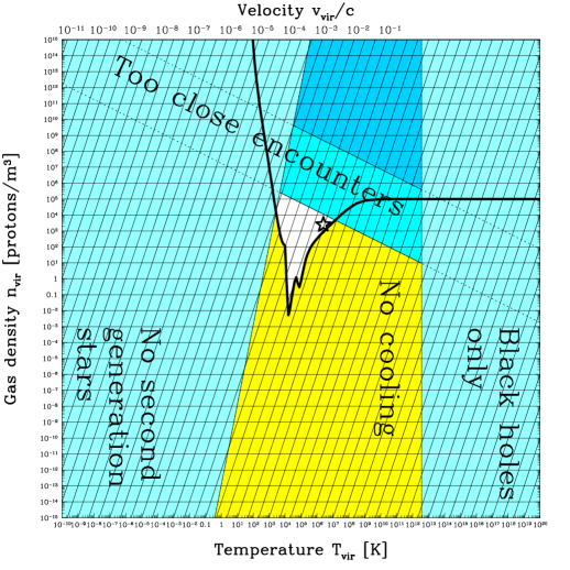
Figure 2: Many selection effects that we discuss are conveniently summarized in the plane tracking the virial temperatures and densities in dark matter halos. The gas cooling requirement prevents halos below the heavy black curve from forming galaxies. Close encounters make stable solar systems unlikely above the downward-sloping line. Other dangers include collapse into black holes and disruption of galaxies by supernova explosions. The location and shape of the small remaining region (unshaded) is independent of all cosmological parameters except the baryon fraction.

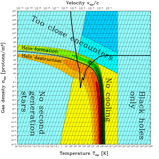
Figure 3: Same as the previous figure, but including the banana-shaped contours showing the the halo formation/destruction rate. Solid/greenish contours correspond to positive net rates (halo production) at 0.5, 0.3, 0,2, 0.1, 0.03 and 0.01 of maximum, whereas dashed/reddish contours correspond to negative net rates (halo destruction from merging) at -0.3, -0,2, -0.1, -0.03 and -0.01 of maximum, respectively. The heavy black contour corresponds to zero net formation rate. The cosmological parameters $(\xi_{\rm b},\xi_{\rm c},\xi_{\nu},,Q,\rho_{\Lambda})$ have a strong effect on this banana: $\xi_{\rm b}$ and $\xi_{\rm c}$ shift this banana-shape vertically, $Q$ shifts if along the parallel diagonal lines and $\rho_{\Lambda}$ cuts it off below $16\rho_{\Lambda}$ (see the next figure). Roughly speaking, there are stable habitable planetary systems only for cosmological parameters where a greenish part of the banana falls within the allowed white region from Figure 2.

We now consider selection effects, by choosing our “selection object” to be a stable solar system, and focusing on requirements for creating these. In line with the preceding discussion, our main interest will be to explore constraints in the 4-dimensional cosmological parameter space $(\xi_{\rm b},\xi_{\rm c},\rho_{\Lambda},Q)$. Since we can only plot one or two dimensions at a time, our discussion will be summarized by a table (Table 4) and a series of figures showing various 1- and 2-dimensional projections: $(\xi_{\rm b},\xi_{\rm c})$, $(\rho_{\Lambda},Q\xi)$, $Q^{3}\xi^{4}$, $\xi$, $\rho_{\Lambda}/Q^{3}\xi^{4}$, $(\xi,Q)$.

Many of the the physical effects that lead to these constraints are summarized in Figure 2 and Figure 3, showing temperatures and densities of galactic halos. The constraints in this plane from galaxy formation and solar system stability depend only on the microphysical parameters $(m_{\rm p},\alpha,\beta)$ and sometimes on the baryon fraction $\xi_{\rm b}/\xi_{\rm c}$, whereas the banana-shaped constraints from dark matter halo formation depend on the cosmological parameters $(\xi_{\rm b},\xi_{\rm c},\xi_{\nu},\rho_{\Lambda},Q)$, so combining them constrains certain parameter combinations. Crudely speaking, $f_{\rm selec}({\bf p})$ will be non-negligible only if the cosmological parameters are such that part of the “banana” falls within the “observer-friendly” (unshaded) region sandwiched between the galaxy formation and solar system stability constraints

In the following three subsections, we will now discuss the three above-mentioned levels of structure formation in turn: halo formation, galaxy formation and solar-system stability.

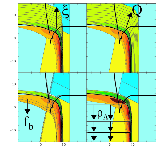
Figure 4: Same as Figure 3, but showing effect of changing the cosmological parameters. Increasing the matter density parameter $\xi$ shifts the banana up by a factor $\xi^{4}$ (top left panel), increasing the fluctuation level $Q$ shifts the banana up by a factor $Q^{3}$ and to the right by a factor $Q$ (top right panel), increasing the baryon fraction $f_{\rm b}=\xi_{\rm b}/\xi$ shifts the banana up by a factor $f_{\rm b}$ and affects the cooling and 2nd generation constraints (bottom left panel), and increasing the dark energy density $\rho_{\Lambda}$ bites off the banana below $\rho_{\rm vir}=16\rho_{\Lambda}$ (bottom right panel). In these these four panels, the parameters have been scaled relative to their observed values as follows: up by $1/4$, $2/4$,…,$9/4$ orders of magnitude ($\xi$), up by $1/3$, $2/3$,…,$9/3$ orders of magnitude ($Q$), down by $1$ and $2$ orders of magnitude ($f_{\rm b}$), and down by $0$, $7$, $12$ and $\infty$ orders of magnitude ($\rho_{\Lambda}$; other panels have $\rho_{\Lambda}=0$).

III.1 Halo formation and the distribution of halo properties

Previous studies (e.g., BarrowTipler ; LindeLambda ; Weinberg87 ; Efstathiou95 ; Vilenkin95 ; Martel98 ; GarrigaVilenkin03 ; inflation ) have computed the total mass fraction collapsed into halos, as a function of cosmological parameters. Here, however, we wish to apply selection effects based on halo properties such as density and temperature, and will compute the formation rate of halos (the banana-shaped function illustrated in Figure 3) in terms of dimensionless parameters alone.

III.1.1 The dependence on mass and time

As previously explained, we will focus on the dark-matter-dominated case $\xi_{\rm c}\gg\xi_{\rm b}$, $\xi_{\rm c}\gg\xi_{\nu}$, so we ignore massive neutrinos and have $\xi=\xi_{\rm b}+\xi_{\rm c}\sim\xi_{\rm c}$. For our calculations, it is convenient to define a new dimensionless time variable

$$x\equiv{\rho_{\Lambda}\over\rho_{\rm m}}={\Omega_{\Lambda}\over\Omega_{m}}={\Omega_{m}^{-1}-1}$$ (12)

and a new dimensionless mass variable

$$\mu\equiv\xi^{2}M.$$ (13)

In terms of the usual cosmological scale factor $a$, our new time variable therefore scales as $x\propto a^{3}$. It equals unity at the vacuum domination epoch when linear fluctuation growth grinds to a halt. The horizon mass at matter-radiation equality is of order $\xi^{-2}$ Q , so $\mu$ can be interpreted as the mass relative to this scale. It is a key physical scale in our problem. It marks the well-known break in the matter power spectrum; fluctuation modes on smaller scales entered the horizon during radiation domination, when they could not grow.

We estimate the fraction of matter collapsed into dark matter halos of mass $M\geq\xi^{-2}\mu$ by time $x$ using the standard Press-Schechter formalism PressSchechter , which gives

$$F(\mu,x)={\mathrm{erfc}}\left[{\delta_{c}(x)\over\sqrt{2}\sigma(\mu,x)}\right].$$ (14)

Here $\sigma(\mu,x)$ is the r.m.s. fluctuation amplitude at time $x$ in a sphere containing mass $M=\xi^{-2}\mu$, so $F$ is the probability that a fluctuation lies $\delta_{c}$ standard deviations out in the tail of a Gaussian distribution. As shown in Appendix A.2, $\sigma$ is well approximated as

$$\sigma(\mu,x)\approx\sigma_{*}{Q\xi^{4/3}\over\rho_{\Lambda}^{1/3}}s(\mu){G_{\Lambda}}(x),$$ (15)

where

$$\sigma_{*}\equiv{45\cdot 2^{1/3}\zeta(3)^{4/3}\over\pi^{14/3}\left[1+{21\over 8}\left({4\over 11}\right)^{4/3}\right]}\approx 0.206271$$ (16)

and the known dimensionless functions $s(\mu)$ and ${G_{\Lambda}}(x)$ do not depend on any physical parameters. $s(\mu)$ and ${G_{\Lambda}}(x)$ give the dependence on scale and time, respectively, and appear in equations (69) and (57) in Appendix A. The scale dependence is $s(\mu)\sim\mu^{-1/3}$ on large scales $\mu\gg 1$, saturating to only logarithmic growth towards small scales for $\mu\ll 1$. Fluctuations grow as ${G_{\Lambda}}(x)\approx x^{1/3}\propto a$ for $x\ll 1$ and then asymptote to a constant amplitude corresponding to ${G_{\infty}}\equiv 5\Gamma\left({2\over 3}\right)\Gamma\left({5\over 6}\right)/3\sqrt{\pi}\approx 1.43728$ as $a\to\infty$ and dark energy dominates. (This is all for $\rho_{\Lambda}>0$; we will treat $\rho_{\Lambda}<0$ in Section III.1.3 and find that our results are roughly independent of the sign of $\rho_{\Lambda}$, so that we can sensibly replace $\rho_{\Lambda}$ by $|\rho_{\Lambda}|$.)

Returning to equation (14), the collapse density threshold $\delta_{c}(x)$ is defined as the linear perturbation theory overdensity that a top-hat-averaged fluctuation would have had at the time $x$ when it collapses. It was computed numerically in anthroneutrino , and found to vary only very weakly (by about 3%) with time, dropping from the familiar cold dark matter value $\delta_{c}(0)=(3/20)(12\pi)^{2/3}\approx 1.68647$ early on to the limit $\delta_{c}(\infty)=(9/5)2^{-2/3}{G_{\infty}}\approx 1.62978$ Weinberg87 in the infinite future. Here we simply approximate it by the latter value:

$$\delta_{c}(x)\approx\delta_{c}(\infty)={9\Gamma\left({2\over 3}\right)\Gamma\left({5\over 6}\right)\over 3\pi^{1/2}2^{2/3}}\approx 1.62978.$$ (17)

Substituting equations (15) and (17) into equation (14), we thus obtain the collapsed fraction

$$F(\mu,x)={\mathrm{erfc}}\left[{A\rho_{\Lambda}^{1/3}\over\xi^{4/3}Q{G_{\Lambda}}(x)s(\mu)}\right],$$ (18)

where

$$A\equiv{\delta_{c}(\infty)\over\sqrt{2}\sigma_{*}}={\left(1+{42\over 22^{4/3}}\right)\pi^{25\over 6}\Gamma\left({2\over 3}\right)\Gamma\left({5\over 6}\right)\over 30\sqrt{2}\zeta(3)^{4/3}}\approx 5.58694.$$ (19)

Below we will occasionally find it useful to rewrite equation (18) as

$$F(\mu,x)={\mathrm{erfc}}\left[{A(\rho_{\Lambda}/\rho_{*})^{1/3}\over{G_{\Lambda}}(x)s(\mu)}\right],\quad\rho_{*}\equiv\xi^{4}Q^{3}.$$ (20)

Let us build some intuition for equation (18). It tells us that early on when $x\sim 0$, no halos have formed ($F\approx 0$), and that as time passes and $x$ increases, small halos form before any large ones since $s(\mu)$ is a decreasing function. Moreover, we see that since ${G_{\Lambda}}(x)$ and $s(\mu)$ are at most of order unity, no halos will ever form if $\rho_{\Lambda}\gg\xi^{4}Q^{3}$. We recognize the combination $\rho_{*}\equiv\xi^{4}Q^{3}$ as the characteristic density of the universe when halos would form in the absence of dark energy Q . If $\rho_{\Lambda}\gg\rho_{*}$, then dark energy dominates long before this epoch and fluctuations never go nonlinear. Figure 5 illustrates that the density distributions corresponding to equation (20) are broadly peaked around $\rho_{\rm vir}\sim 10^{2}\rho_{*}$ when $\rho_{*}\gg\rho_{\Lambda}$, are exponentially suppressed for $\rho_{*}\ll\rho_{\Lambda}$, and in all cases give no halos with $\rho_{\rm vir}<16\rho_{\Lambda}$.

III.1.2 The dependence on temperature and density

Figure 5: Halo density distribution for various values of $\hat{\rho}_{*}/\rho_{\Lambda}$, where $\hat{\rho}_{*}\equiv[s(\mu)/A]^{3}\rho_{*}\sim Q^{3}\xi^{4}$. The dashed curves show the cumulative distribution $F={\mathrm{erfc}}\left[{(\rho_{\Lambda}/\hat{\rho}_{*})^{1/3}/{G_{\Lambda}}(x[\rho_{\rm vir}])}\right]$ and the solid curves show the probability distribution $-\partial F/\partial\lg\rho_{\rm vir}$ for (peaking from right to left) $\hat{\rho}_{*}/\rho_{\Lambda}=10^{5}$, $10^{4}$, $10^{3}$, $10^{2}$, $10$, $1$ (heavy curves), $0.1$ and $0.05$. Note that no halos with $\rho_{\rm vir}<16\rho_{\Lambda}$ are formed.

We now discuss how our halo mass $\mu$ and formation time $x$ transform into the astrophysically relevant parameters $(T_{\rm vir},n_{\rm vir})$ appearing in Figure 3.

As shown in Appendix A.3, halos that virialize at time $x$ have a characteristic density of order

$$\rho_{\rm vir}\sim 16\rho_{\Lambda}\left[\left({9\pi^{2}\over 8x}\right)^{107\over 200}+1\right]^{200\over 107},$$ (21)

i.e., essentially the larger of the two terms $16\rho_{\Lambda}$ and $18\pi^{2}\rho_{\rm m}(x)$. For a halo of total (baryonic and dark matter) mass $M$ in Planck units, this corresponds to a characteristic size $R\sim(M/\rho_{\rm vir})^{1/3}$, velocity $v_{\rm vir}\sim(M/R)^{1/2}\sim(M^{2}\rho_{\rm vir})^{1/6}$ and virial temperature $T_{\rm vir}\sim m_{p}v_{vir}^{2}\sim m_{\rm p}M^{2/3}\rho_{\rm vir}^{1/3}$, so

$$T_{\rm vir}\sim m_{p}\left({16\rho_{\Lambda}\mu^{2}\over\xi^{4}}\right)^{1/3}\left[\left({9\pi^{2}\over 8x}\right)^{107\over 200}+1\right]^{200\over 321}.$$ (22)

Inverting equations (21) and (22) gives

$$\mu \sim \sqrt{\xi^{4}T_{\rm vir}^{3}\over m_{p}^{3}\rho_{\rm vir}},$$ (23)

$$x \sim {9\pi^{2}\over 8}\left[\left({\rho_{\rm vir}\over 16\rho_{\Lambda}}\right)^{107\over 200}-1\right]^{-{200\over 107}}.$$ (24)

For our applications, the initial gas temperature will be negligible and the gas density will trace the dark matter density, so until cooling becomes important (Section III.2.1), the proton number density is simply

$$n_{\rm vir}={\xi_{\rm b}\over\xi m_{\rm p}}\rho_{\rm vir}.$$ (25)

According to the Press-Schechter approximation, the derivative $-{\partial F\over\partial\lg\mu}(\mu,x)$ can be interpreted as the so-called mass function, i.e., as the distribution of halo masses at time $x$. We can therefore interpret the second derivative

$$f_{\mu x}(\mu,x)\equiv-{\partial^{2}F\over\partial(\lg\mu)\partial(\lg x)}$$ (26)

as the net formation rate of halos as a function of mass and time. Transforming this rate from $(\lg\mu,\lg x)$-space to $(\lg T_{\rm vir},\lg\rho_{\rm vir})$-space, we obtain the function whose banana-shaped contours are shown in Figure 3:

$$f(T_{\rm vir},n_{\rm vir})\equiv|J|f_{\mu x}(\mu,x)=|J|{\partial^{2}F\over\partial(\lg\mu)\partial(\lg x)},$$ (27)

where $J$ is a Jacobian determinant that can be ignored safely.

Let us now build some intuition for this important function $f(T_{\rm vir},n_{\rm vir})$. First of all, since equation (21) shows that $\rho_{\rm vir}\propto n_{\rm vir}$ decreases with time and is $\mu$-independent, we can reinterpret the vertical $n_{\rm vir}$-axis in Figure 3 as simply the time axis: as our Universe expands, halos can form at lower densities further and further down in the plot. Since nothing ever forms with $\rho_{\rm vir}<16\rho_{\Lambda}$, the horizontal line $n_{\rm vir}=16\rho_{\Lambda}\xi_{\rm b}/\xi m_{\rm p}$ corresponds to $t\to\infty$. Second, $f$ is the net formation rate, which means that it is negative if the rate of formation of new halos of this mass is smaller than the rate of destruction from merging into larger halos. The destruction stems from the fact that, to avoid double-counting, the Press-Schechter approximation counts a given proton as belonging to at most one halo at a given time, defined as the largest nonlinear structure that it is part of. Figure 3 shows that halos of any given mass (defined by the lines of slope 3) are typically destroyed in this fashion some time after its formation unless $\rho_{\Lambda}$-domination terminates the process of fluctuation growth.

We will work out the detailed dependence of this banana on physical parameters in the next section. For now, we merely note that Figure 3 shows that the first halos form with characteristic density $\rho_{\rm vir}\sim\rho_{*}\sim\xi^{4}Q^{3}$, $n_{\rm vir}\sim\xi_{\rm b}\xi^{3}Q^{3}/m_{\rm p}$, and (assuming $\rho_{\Lambda}\ll\rho_{*}$) the largest halos approach virial velocities $v_{\rm vir}\sim Q^{1/2}c$ and temperatures $T_{\rm vir}\sim Q\times m_{\rm p}c^{2}$ Q .

III.1.3 How $m_{\rm p}$, $\xi_{\rm b}$, $\xi_{\rm c}$, $Q$ and $\rho_{\Lambda}$ affect “the banana”

Substituting the preceding equations into equation (27) gives the explicit expression

$$f(T_{\rm vir},n_{\rm vir};m_{\rm p},\xi_{\rm b},\xi_{\rm c},Q,\rho_{\Lambda})=$$

$$={3a\left[{G_{\Lambda}}(x)^{2}s(\mu)^{2}-2a^{2}\right]x{G_{\Lambda}}^{\prime}(x)\mu s^{\prime}(\mu)\over\sqrt{\pi}{G_{\Lambda}}(x)^{4}s(\mu)^{4}\exp\left[\left({a\over{G_{\Lambda}}(x)s(\mu)}\right)^{2}\right]}\left({\rho_{\rm vir}x\over 18\pi^{2}\rho_{\Lambda}}\right)^{159\over 200},$$

$$a\equiv{A\rho_{\Lambda}^{1/3}\over Q\xi^{4/3}},$$ (30)

where $\mu$ and ${\bf x}$ are determined by $T_{\rm vir}$ and $n_{\rm vir}$ via equations (23),  (24) and  (25). This is not very illuminating. We will now see how this complicated-looking function $f$ of seven variables can be well approximated and understood as a fixed banana-shaped function of merely two variables, which gets translated around by variation of $m_{\rm p}$, $\xi_{\rm b}$, $\xi_{\rm c}$ and $Q$, and truncated from below at a value determined by $\rho_{\Lambda}$.

Let us first consider the limit $\rho_{\Lambda}\to 0$ where dark energy is negligible. Then $x\ll 1$ so that ${G_{\Lambda}}(x)=x^{1/3}=(\rho_{\Lambda}/\rho_{\rm m})^{1/3}$, causing equation (18) to simplify to

$$F(\mu,x)={\mathrm{erfc}}\left[{A\rho_{\rm m}^{1/3}\over\xi^{4/3}Qs(\mu)}\right].$$ (31)

In the same limit, equation (21) reduces to $\rho_{\rm vir}=18\pi^{2}\rho_{\rm m}$, so using equation (25) gives $\rho_{\rm m}=\rho_{\rm vir}/18\pi^{2}=\xi m_{\rm p}n_{\rm vir}/18\pi^{2}\xi_{\rm b}$. Using this and equation (23), we can rewrite equation (31) in the form

$$F = {\mathrm{erfc}}\left[{A\left({m_{\rm p}n_{\rm vir}\over\xi_{\rm b}\xi^{3}Q^{3}}\right)^{1/3}\over\left(18\pi^{2}\right)^{1/3}s\left[\left({T_{\rm vir}\over m_{\rm p}Q}\right)^{3/2}\left({m_{\rm p}n_{\rm vir}\over\xi_{\rm b}\xi^{3}Q^{3}}\right)^{-1/2}\right]}\right]$$ (32)

$$= B\left({m_{\rm p}n_{\rm vir}\over\xi_{\rm b}\xi^{3}Q^{3}},{T_{\rm vir}\over m_{\rm p}Q}\right),$$

where the “standard banana” is characterized by a function of only two variables,

$$B(X,Y)={\mathrm{erfc}}\left[{AX^{1/3}\over\left(18\pi^{2}\right)^{1/3}s\left[Y^{3/2}X^{-1/2}\right]}\right].$$ (33)

Thus $B(X,Y)$ determines the banana shape, and the parameters $m_{\rm p}$, $\xi_{\rm b}$, $\xi$ and $Q$ merely shift it on a log-log plot: increasing $m_{\rm p}$ shifts it down and to the right along lines of slope $-1$, increasing $\xi_{\rm b}$ shifts it upward, increasing $\xi$ shifts it upward three times faster, and increasing $Q$ shifts it upward and to the right along lines of slope $3$. The halo formation rate defined by its derivatives (equation 27) and plotted in Figure 3 clearly scales in exactly the same way with these four parameters, since in the $\rho_{\Lambda}\to 0$ limit that we are considering, the Jacobian ${\bf J}$ is simply a constant matrix.

Let us now turn to the general case of arbitrary $\rho_{\Lambda}$. As as discussed above, time runs downward in Figure 3 since the cosmic expansion gradually dilutes the matter density $\rho_{\rm m}$. The matter density completely dwarfs the dark energy density at very early times. They key point is that since $\rho_{\Lambda}$ has no effect until our Universe has expanded enough for the matter density to drop near the dark energy density, the part of the banana in Figure 3 that lies well above the vacuum density $\rho_{\Lambda}$ will be completely independent of $\rho_{\Lambda}$. As the matter density $\rho_{\rm m}$ drops below $\rho_{\Lambda}$ (i.e., as $x$ grows past unity), fluctuation growth gradually stops. This translates into a firm cutoff below $\rho_{\rm vir}=16\rho_{\Lambda}$ in Figure 3 (i.e., below $n_{\rm vir}=16\xi_{\rm b}\rho_{\Lambda}/m_{\rm p}\xi$), since equation (21) shows that no halos ever form with densities below that value.

Viewed at sensible resolution on our logarithmic plot, spanning many orders of magnitude in density, the transition from weakly perturbing the banana to biting it off is quite abrupt, occurring as the density changes by a factor of a few. For the purposes of this paper, it is appropriate to approximate the effect of $\rho_{\Lambda}$ as simply truncating the banana below the cutoff density.

Putting it together, we can approximate the non-intuitive equation (III.1.3) by the much simpler

$$f(T_{\rm vir},n_{\rm vir};m_{\rm p},\xi_{\rm b},\xi_{\rm c},Q,\rho_{\Lambda})\approx$$

$$\approx b\left({T_{\rm vir}\over m_{p}Q},{m_{\rm p}n_{\rm vir}\over\xi_{\rm b}\xi^{3}Q^{3}}\right)\theta\left(n_{\rm vir}-{16\xi_{\rm b}\rho_{\Lambda}\over m_{\rm p}\xi}\right),$$ (34)

where $\theta$ is the Heaviside step function ($\theta(x)=0$ for $x<0$, $\theta(x)=1$ for $x\geq 0$) and $b$ is the differentiated “standard banana” function

$$b(X,Y)\equiv{\partial^{2}\over\lg X\lg Y}B(X,Y).$$ (35)

This is useful for understanding constraints on the cosmological parameters: the seemingly complicated dependence of the halo distribution on seven variables from equation (III.1.3) can be intuitively understood as the standard banana shape from Figure 3 being rigidly translated by the four parameters $m_{\rm p}$, $\xi_{\rm b}$, $\xi$ and $Q$ and truncated from below with a cutoff $n_{\rm vir}>16\xi_{\rm b}\rho_{\Lambda}/m_{\rm p}\xi$. All this is illustrated in Figure 4, which also confirms numerically that the approximation of equation (35) is quite accurate.

III.1.4 The case $\rho_{\Lambda}<0$

Above we assumed that $\rho_{\Lambda}\geq 0$, but for the purposes of this paper, we can obtain a useful approximate generalization of the results by simply replacing $\rho_{\Lambda}$ by $|\rho_{\Lambda}|$ in equation (III.1.3). This is because $\rho_{\Lambda}$ has a negligible effect early on when $|\rho_{\Lambda}|\ll\rho_{m}$ and a strongly detrimental selection effect when $|\rho_{\Lambda}|\sim\rho_{m}$, either by suppressing galaxy formation (for $\rho_{\Lambda}>0$) or by recollapsing our universe (for $\rho_{\Lambda}<0$), in either case causing a rather sharp lower cutoff of the banana. As pointed out by Weinberg Weinberg87 , one preferentially expects $\rho_{\Lambda}>0$ as observed because the constraints tend to be slightly stronger for negative $\rho_{\Lambda}$. If $\rho_{\Lambda}>0$, observers have time to evolve long after $|\rho_{\Lambda}|=\rho_{\rm m}$ as long as galaxies had time to form before while $\rho_{\Lambda}$ was still subdominant. If $\rho_{\Lambda}<0$, however, both galaxy formation and observer evolution must be completed before $\rho_{\Lambda}$ dominates and recollapses the universe; thus, for example, increasing $Q$ so as to make structure form earlier will not significantly improve prospects for observers.

III.2 Galaxy formation

III.2.1 Cooling and disk formation

Above we derived the time-dependent (or equivalently, density-dependent) fraction of matter collapsed into halos above a given mass (or temperature), derived from this the formation rate of halos of a given temperature and density, and discussed how both functions depended on cosmological parameters. For the gas in such a halo to be able to contract and form a galaxy, it must be able to dissipate energy by cooling Binney77 ; ReesOstriker77 ; WhiteRees78 ; Blanchard92 — see RipamontiAbel05 for a recent review. In the shaded region marked “No cooling” in Figure 2, the cooling timescale $T/\dot{T}$ exceeds the Hubble timescale $H^{-1}$. We have computed this familiar cooling curve as in Q with updated molecular cooling from Tom Abel’s code based on GalliPalla98 , which is available at http://www.tomabel.com/PGas/. From left to right, the processes dominating the cooling curve are molecular hydrogen cooling (for $T\mathrel{\hbox to0.0pt{\lower 3.0pt\hbox{$\mathchar 536\relax$}\hss}\raise 2.0pt\hbox{$\mathchar 316\relax$}}10^{4}$K), hydrogen line cooling (1st trough), helium line cooling (2nd trough), Bremsstrahlung from free electrons (for $T\mathrel{\hbox to0.0pt{\lower 3.0pt\hbox{$\mathchar 536\relax$}\hss}\raise 2.0pt\hbox{$\mathchar 318\relax$}}10^{5}$K) and Compton cooling against cosmic microwave background photons (horizontal line for $T\mathrel{\hbox to0.0pt{\lower 3.0pt\hbox{$\mathchar 536\relax$}\hss}\raise 2.0pt\hbox{$\mathchar 318\relax$}}10^{9}$K). The curve corresponds to zero metallicity, since we are interested in whether the first galaxies can form.

The cooling physics of course depends only on atomic processes, i.e., on the three parameters $(\alpha,\beta,m_{\rm p})$. Requiring the cooling timescale to not exceed some fixed timescale would therefore give a curve independent of all cosmological parameters. Since we are instead requiring the cooling timescale ($\propto n^{-1}$ for all processes involving particle-particle collisions) not to exceed the Hubble timescale ($\propto\rho_{\rm m}^{-1/2}\propto(n/f_{\rm b})^{-1/2}$), our cooling curve will depend also on the baryon fraction $f_{b}$, with all parts except the Compton piece to the right scaling vertically as $f_{\rm b}^{-1}$.

III.2.2 Disk fragmentation and star formation

We have now discussed how fundamental parameters determine whether dark matter halos form and whether gas in such halos can cool efficiently. If both of these conditions are met, the gas will radiate away kinetic energy and settle into a rotationally supported disk, and the next question becomes whether this disk is stable or will fragment and form stars. As described below, this depends strongly on the baryon fraction $f_{\rm b}\equiv\xi_{\rm b}/\xi$, observed to be $f_{\rm b}\sim 1/6$ in our universe. The constraints from this requirement propagate directly into Figure 12 in Section IV.4 rather than Figure 3.

First of all, stars need to have a mass of at least ${M_{\rm min}}\approx 0.08M_{\odot}$ for their core to be hot enough to allow fusion. Requiring the formation of at least one star in a halo of mass $M$ therefore gives the constraint

$$f_{\rm b}>{{M_{\rm min}}\over M}.$$ (36)

An interesting point HellermanWalcher05 is that this constraint places an upper bound on the dark matter density parameter. Since the horizon mass at equality is $M_{\rm eq}\sim\xi^{-2}$ Q , the baryon mass within the horizon at equality is $M_{\rm eq}\xi_{\rm b}/\xi\sim\xi_{\rm b}/\xi^{3}$, which drops with increasing $\xi$. This scale corresponds to the bend in the banana of Figure 3, so unless HellermanWalcher05

$$f_{\rm b}\mathrel{\hbox to0.0pt{\lower 3.0pt\hbox{$\mathchar 536\relax$}\hss}\raise 2.0pt\hbox{$\mathchar 318\relax$}}{{M_{\rm min}}\xi^{2}},$$ (37)

one needs to wait until long after the first wave of halo formation to form the first halo containing enough gas to make a star, which in turn requires a correspondingly small $\rho_{\Lambda}$-value. The ultimate conservative limit is requiring that $M_{\rm b}^{\rm h}\sim\rho_{\rm b}H^{-3}$, the baryon mass within the horizon, exceeds ${M_{\rm min}}$. Since $M_{\rm b}^{\rm h}$ increases during matter domination and decreases during vacuum domination, taking its maximum value $M_{\rm b}^{\rm h}\sim f_{\rm b}\rho_{\Lambda}^{-1/2}$ when $x\sim 1$, the $M_{\rm b}^{\rm h}>{M_{\rm min}}$ requirement gives

$$f_{\rm b}\mathrel{\hbox to0.0pt{\lower 3.0pt\hbox{$\mathchar 536\relax$}\hss}\raise 2.0pt\hbox{$\mathchar 318\relax$}}{{M_{\rm min}}\rho_{\Lambda}^{1/2}}.$$ (38)

However, these upper limits on the dark matter parameter density parameter $\xi_{\rm c}$ are very weak: for the observed values of $\xi_{\rm b}$ and $\rho_{\Lambda}$ from Table 1, equations (37) and (38) give $\xi_{\rm c}<\xi\mathrel{\hbox to0.0pt{\lower 3.0pt\hbox{$\mathchar 536\relax$}\hss}\raise 2.0pt\hbox{$\mathchar 316\relax$}}(\xi_{\rm b}/{M_{\rm min}})^{1/3}\sim 10^{-22}$ and $\xi_{\rm c}<\xi\mathrel{\hbox to0.0pt{\lower 3.0pt\hbox{$\mathchar 536\relax$}\hss}\raise 2.0pt\hbox{$\mathchar 316\relax$}}\xi_{\rm b}/{M_{\rm min}}\rho_{\Lambda}^{1/2}\sim 10^{-4}$, respectively, limits many orders of magnitude above the observed value $\xi_{\rm c}\sim 10^{-28}$.

It seems likely, however, that ${M_{\rm min}}$ is a gross underestimate of the baryon requirement for star formation. The fragmentation instability condition for a baryonic disc is essentially that it should be self-gravitating in the “vertical” direction. This is equivalent to requiring the baryonic density in the disc exceed that of the dark matter background it is immersed in. The first unstable mode is then the one that induces breakup into spheres of radius of order the disc thickness. This conservative criterion is weaker than the classic Toomre instability criterion Toomre64 , which requires the disc to be self-gravitating in the radial direction and leads to spiral arm formation. If the halo were a singular isothermal sphere, then FallEfstathiou80 instability would require

$$f_{\rm b}\mathrel{\hbox to0.0pt{\lower 3.0pt\hbox{$\mathchar 536\relax$}\hss}\raise 2.0pt\hbox{$\mathchar 318\relax$}}\lambda\left({{T_{\rm min}}\over T_{\rm vir}}\right)^{1/2},$$ (39)

Here ${T_{\rm min}}$ is the minimum temperature that the gas can cool to and $\lambda$ is the dimensionless specific angular momentum parameter, which has an approximately lognormal distribution centered around 0.08 FallEfstathiou80 . For an upper limit on the dark matter parameter $\xi_{\rm c}$, what matters is thus the upper limit on $\lambda$, the upper limit on $T_{\rm vir}$ and the lower limit on ${T_{\rm min}}$, all three of which are quite firm. Ignoring probability distributions, taking ${T_{\rm min}}\sim\alpha^{2}\beta m_{\rm p}/6\ln\alpha^{-1}\sim 10^{4}{\rm K}\sim 1\ {\rm eV}$ (atomic Hydrogen line cooling) and $T_{\rm vir}\sim 500{\rm eV}$ (Milky Way) gives $T_{\rm vir}/{T_{\rm min}}\sim 500$, $\xi_{\rm c}\mathrel{\hbox to0.0pt{\lower 3.0pt\hbox{$\mathchar 536\relax$}\hss}\raise 2.0pt\hbox{$\mathchar 316\relax$}}300\xi_{\rm b}$ from equation (39). Taking the extreme values ${T_{\rm min}}\sim 500{\rm K}$ ($H_{2}$-cooling freezeout) and $T_{\rm vir}\sim m_{\rm p}Q\sim 20$ keV (largest clusters) gives $T_{\rm vir}/{T_{\rm min}}\sim 10^{10}Q$ and $\xi\mathrel{\hbox to0.0pt{\lower 3.0pt\hbox{$\mathchar 536\relax$}\hss}\raise 2.0pt\hbox{$\mathchar 316\relax$}}10^{6}Q^{1/2}\xi_{\rm b}\sim 10^{4}\xi_{\rm b}$. On the other extreme, if we argue that $T_{\rm vir}\sim{T_{\rm min}}$ for the very first galaxies to form, then equation (39) gives $\xi/\xi_{\rm b}\mathrel{\hbox to0.0pt{\lower 3.0pt\hbox{$\mathchar 536\relax$}\hss}\raise 2.0pt\hbox{$\mathchar 316\relax$}}12$, which is interestingly close to what we observe.

For NFW potentials NFW , $\lambda$-dependence is more complicated and the local velocity dispersion of the dark matter near the center is lower than the mean $T_{\rm vir}$.

Even if the baryon fraction were below the threshold of equation (39), stars could eventually form because viscosity (even just “molecular” viscosity) would redistribute mass and angular momentum so that the gas becomes more centrally condensed. The condition then becomes that the mass of spherical blob of radius $R\sim M_{\rm d}/{T_{\rm min}}$ exceed the dark mass $M_{\rm d}$ within that radius. For the isothermal sphere, this would automatically happen, but for a realistic flat-bottomed or NFW potential, then this gives a non-trivial inequality. For instance, in a parabolic potential well, the requirement would be that

$$f_{\rm b}\mathrel{\hbox to0.0pt{\lower 3.0pt\hbox{$\mathchar 536\relax$}\hss}\raise 2.0pt\hbox{$\mathchar 318\relax$}}\left({{T_{\rm min}}\over T_{\rm vir}}\right)^{3/2}.$$ (40)

Although a weaker limit limit than equation (39), giving $\xi_{\rm c}\mathrel{\hbox to0.0pt{\lower 3.0pt\hbox{$\mathchar 536\relax$}\hss}\raise 2.0pt\hbox{$\mathchar 316\relax$}}10^{4}\xi_{\rm b}$ for the above example with $T_{\rm vir}/{T_{\rm min}}\sim 500$, it is still stronger than those of equation (37) and equation (38). A detailed treatment of these issues is beyond the scope of the present paper; it should include modeling of the $t\to\infty$ limit as well as merger-induced star formation and the effect of dark matter substructure disturbing and thickening the disk.

III.3 Second generation star formation

Suppose that all the above conditions have been met so that a halo has formed where gas has cooled and produced at least one star. The next question becomes whether the heavy elements produced by the death of the first star(s) can be recycled into a solar system around a second generation star, thereby allowing planets and perhaps observers made of elements other than hydrogen, helium and the trace amounts of deuterium and lithium left over from big bang nucleosynthesis.

The first supernova explosion in the halo will release not only heavy metals, but also heat energy of order

$$E=10^{-3}m_{\rm p}^{-2}\sim 10^{46}\hbox{J}=10^{51}\hbox{erg}.$$ (41)

Here $m_{\rm p}^{-2}$ is the approximate binding energy of a Chandrashekar mass at its Schwarzschild radius, with the prefactor incorporating the fact that neutron stars are usually somewhat larger and heavier and, most importantly, that about 99% of the binding energy is lost in the form of neutrinos.

By the virial theorem, the gravitational binding energy $E$ of the halo equals twice its total kinetic energy, i.e.,

$$E\approx Mv_{\rm vir}^{2}\sim\sqrt{T_{\rm vir}^{5}\over m_{\rm p}^{5}\rho_{\rm vir}},$$ (42)

where we have used equation (23) in the last step. If ${E_{\rm sn}}\gg E$, the very first supernova explosion will therefore expel essentially all the gas from the halo, precluding the formation of second generation stars. Combining equations (41) and (42), we therefore obtain the constraint

$$\rho_{\rm vir}\mathrel{\hbox to0.0pt{\lower 3.0pt\hbox{$\mathchar 536\relax$}\hss}\raise 2.0pt\hbox{$\mathchar 316\relax$}}10^{6}{T_{\rm vir}^{5}\over m_{\rm p}}.$$ (43)

Figure 2 illustrates this fact that lines of constant binding energy have slope 5, and shows that the second generation constraint rules out an interesting part of the the $(n_{\rm vir},T_{\rm vir})$ plane that is allowed by both cooling and disruption constraints.

While we have ignored the important effect of cooling by gas in the supernova’s immediate environment, this constraint is probably nonetheless rather conservative, and a more detailed calculation may well move it further to the right. First of all, many supernovae tend to go off in close succession in a star formation site, thereby jointly releasing more energy than indicated by equation (42). Second, it is likely that many supernovae are required to produce sufficiently high metallicity. Since $\sim 1$ supernova forms per $100M_{\odot}$ of star formation, releasing $\sim 1M_{\odot}$ of metals, raising the mean metallicity in the halo to solar levels ($\sim 10^{-2}$) would require an energy input of order $E/(100m_{\star}/m_{\rm p})\sim 10^{-5}m_{\rm p}\sim 10\,$keV per proton. A careful calculation of the corresponding temperature would need to model the gas cooling occurring between the successive supernova explosions.

III.4 Encounters and extinctions

The effect of halo density on solar system destruction was discussed in Q making the crude assumption that all halos of a given density had the same characteristic velocity dispersion. Let us now review this issue, which will play a key role in determining predictions for the axion density, from the slightly more refined perspective of Figure 2. Consider a habitable planet orbiting a star of mass $M$ suffering a close encounter with another star of mass $M_{\dagger}$, approaching with a relative velocity $v_{\dagger}$ and an impact parameter $b$. There is some “kill” cross section $\sigma_{\dagger}(M,M_{\dagger},v_{\dagger})=\pi b^{2}$ corresponding to encounters close enough to make this planet uninhabitable. There are several mechanisms through which this could happen:

1. It could become gravitationally unbound from its parent star, thereby losing its key heat source.

2. It could be kicked into a lethally eccentric orbit.

3. The passing star could cause disastrous heating.

4. The passing star could perturb an Oort cloud in the outer parts of the solar system, triggering a lethal comet impact.

The probability of the planet remaining unscathed for a time $t$ is then $e^{-\gamma_{\dagger}t}$, where the destruction rate is $\gamma_{\dagger}$ is $n_{\star}\sigma_{\dagger}v_{\dagger}$ appropriately averaged over incident velocities $v_{\dagger}$ and stellar masses $M$ and $M_{\dagger}$. Assuming that $n_{\star}\propto n_{\rm vir}$, $v_{\dagger}\propto v_{\rm vir}\propto T_{\rm vir}^{1/2}$ and $\sigma_{\dagger}$ is independent of $n_{\rm vir}$ and $T_{\rm vir}$, contours of constant destruction rate in Figure 2 are thus lines of slope $-1/2$. The question of which such contour is appropriate for our present discussion is highly uncertain, and deserving of future work that would lie beyond the scope of the present paper. Below we explore only a couple of crude estimates, based on direct and indirect impacts, respectively.

III.4.1 Direct encounters

Lightman Lightman84 has shown that if the planetary surface temperature is to be compatible with life as we know it, the orbit around the central star should be fairly circular and have a radius of order

$$r_{\rm au}\sim\alpha^{-5}m_{\rm p}^{-3/2}\beta^{-2}\sim 10^{11}{\rm m},$$ (44)

roughly our terrestrial “astronomical unit”, precessing one radian in its orbit on a timescale

$$t_{orb}\sim\alpha^{-15/2}m_{\rm p}^{-5/4}\beta^{-3}\sim 0.1\hbox{ year}.$$ (45)

An encounter with another star with impact parameter $r\mathrel{\hbox to0.0pt{\lower 3.0pt\hbox{$\mathchar 536\relax$}\hss}\raise 2.0pt\hbox{$\mathchar 316\relax$}}r_{\rm au}$ has the potential to throw the planet into a highly eccentric orbit or unbind it from its parent star. For $n_{\star}$, what matters here is not the typical stellar density in a halo, but the stellar density near other stars, including the baryon density enhancement due to disk formation and subsequent fragmentation. Let us write

$$n_{\star}={f_{\star}n_{\rm vir}\over N_{\star}},$$ (47)

where $N_{\star}\sim m_{\rm p}^{-3}\sim 10^{57}$ is the number of protons in a star and the dimensionless factor $f_{\star}$ parametrizes our uncertainty about the extent to which stars concentrate near other stars. Substituting characteristic values $n_{\rm vir}\sim 10^{3}/m^{3}$ for the Milky Way and $n_{\star}\sim(1\,{\rm pc})^{-3}$ for the solar neighborhood gives a concentration factor $f_{\star}\sim 10^{5}$. Using this value, $v_{\dagger}\sim v_{\rm vir}$ and $\sigma_{\dagger}=\pi r_{\rm au}^{2}$ excludes the dark shaded region to the upper right in Figure 2 if we require $\gamma_{\dagger}^{-1}$ to exceed $t_{\rm min}\sim 10^{9}$ years $\sim\alpha^{2}\alpha_{g}^{-3/2}\beta^{-2}$, the lifetime of a bright star CarrRees79 . It is of course far from clear what is an appropriate evolutionary or geological timescale to use here, and there are many other uncertainties as well. It is probably an overestimate to take $v_{\dagger}\sim v_{\rm vir}$ since we only care about relative velocities. On the other hand, our value of $\sigma_{\dagger}$ is an underestimate since we have neglected gravitational focusing. The value we used for $f_{\star}$ is arguably an underestimate as well, stellar densities being substantially higher in giant molecular clouds at the star formation epoch.

III.4.2 Indirect encounters

In the above-mentioned encounter scenarios 1-3, the incident directly damages the habitability of the planet. In scenario 4, the effect is only indirect, sending a hail of comets towards the inner solar system which may at a later time impact the planet. This has been argued to place potentially stronger upper limits on $Q$ than direct encounters GarrigaVilenkin05 .

Although violent impacts are commonplace in our particular solar system, large uncertainties remain in the statistical details thereof and in the effect that changing $n_{\star}$ and $v_{\dagger}$ would have. It is widely believed that solar systems are surrounded by a rather spherical cloud of comets composed of ejected leftovers. Our own particular Oort cloud is estimated to contain of order $10^{12}$ comets, extending out to about a lightyear ($\sim 10^{5}$AU) from the Sun. Recent estimates suggest that the impact rate of Oort cloud comets exceeding 1 km in diameter is between 5 and 700 per million years Nurmi01 . These impacts are triggered by gravitational perturbations to the Oort cloud sending a small fraction of the comets into the inner solar system. About 90% of these perturbations are estimated to be caused by Galactic tidal forces (mainly related to the motion of the Sun with respect to the Galactic midplane), with random passing stars being responsible for most of the remainder and random passing molecular clouds playing a relatively minor role Byl83 ; Hut97 ; Nurmi01 .

It is well-known that Earth has suffered numerous violent impacts with celestial bodies in the the past, and the 1994 impact of comet Shoemaker-Levy on Jupiter illustrated the effect of comet impacts. Although the nearly 10 km wide asteroid that hit the Yucatan 65 million years ago Alvarez80 may actually have helped our own evolution by eliminating dinosaurs, a larger impact of a 30 km object 3.47 billion years ago Byerly02 may have caused a global tsunami and massive heating, killing essentially all life on Earth (For comparison, the Shoemaker-Levy fragments were less than 2 km in size.) We therefore cannot dismiss out of hand the possibility that we are in fact close to the edge in parameter space, with only a modest increase in comet impact rates on planets causing a significant drop in the fraction of planets evolving observers. This possibility is indicated by the light-shaded excluded region in the upper right of Figure 2.

However, there are large uncertainties here of two types. First, we lack accurate risk statistics for our own particular solar system. Although the lunar crater radius distribution is roughly power law of slope $-2$ at high end, we still have very limited knowledge of the size distribution of comet nuclei Meech04 and hence cannot accurately estimate the frequency of extremely massive impacts. Second, we lack accurate estimates of what would happen in denser galaxies. There, the more frequent close encounters with other stars could rapidly strip stars of much of their dangerous Oort cloud, so it is far from obvious that the risk rises as $n_{\star}v_{\dagger}$. One interesting possibility is that the inner Oort cloud at radii $\mathrel{\hbox to0.0pt{\lower 3.0pt\hbox{$\mathchar 536\relax$}\hss}\raise 2.0pt\hbox{$\mathchar 316\relax$}}1000$AU contributes a substantial fraction of our impact risk, in which case such tidal stripping of most of the cloud by volume will do little to reduce risk.

An indirect hint that comet impacts are anthropically important may be the observation Gonzalez99 that the orbit of our Sun through the galaxy appears fine-tuned to minimize Oort cloud perturbations and resulting comet impacts: compared to similar stars, its orbit has an unusually low eccentricity and small amplitude of vertical motion relative to the Galactic disk.

III.4.3 Nearby explosions

A final category of risk that deserves further exploration is that from nearby supernova explosions and gamma-ray bursts. Since these are independent of stellar motion and thus depend only on $n_{\star}$, not on $T_{\rm vir}$, they would correspond to a horizontal upper cutoff in Figure 2. For example, the Ordovician extinction 440 million years ago has been blamed on a nearby gamma-ray burst. This would have depleted the ozone layer causing a massive increase in ultraviolet solar radiation exposure and could also have triggered an ice age Melott05 .

III.5 Black hole formation

There are two potentially rather extreme selection effects involving black holes.

First, Figure 2 illustrates a vertical constraint on the right side corresponding to large $T_{\rm vir}$-values. Since the right edge of the halo banana is at $v_{\rm vir}\sim Q^{1/2}c$, typical halos will form black holes for $Q$-values of order unity as discussed in Q . Specifically, typical fluctuations would be of black-hole magnitude already by the time they entered the horizon, converting some substantial fraction of the radiation energy into black holes shortly after the end of inflation and continually increasing this fraction as longer wavelength fluctuations entered and collapsed. For a scale-invariant spectrum, extremely rare fluctuations that are $Q^{-1}$ standard deviations out in the Gaussian tail can cause black hole domination if Q

$$Q\mathrel{\hbox to0.0pt{\lower 3.0pt\hbox{$\mathchar 536\relax$}\hss}\raise 2.0pt\hbox{$\mathchar 318\relax$}}10^{-1}.$$ (48)

This constraint is illustrated in Figure 12 below rather than in Figure 3.

A second potential hazard occurs if halos form with high enough density that collapsing gas can trap photons. This makes the effective $\gamma$-factor close to 4/3 so that the Jeans mass does not fall as collapse proceeds, and collapse proceeds in a qualitatively different way because there will be no tendency to fragment. This might lead to production of single black hole (instead of a myriad of stars) or other pathological objects, but what actually happens would depend on unknown details, such as whether angular momentum can be transported outward so as to prevent the formation of a disk.

III.6 Constraints related to the baryon density

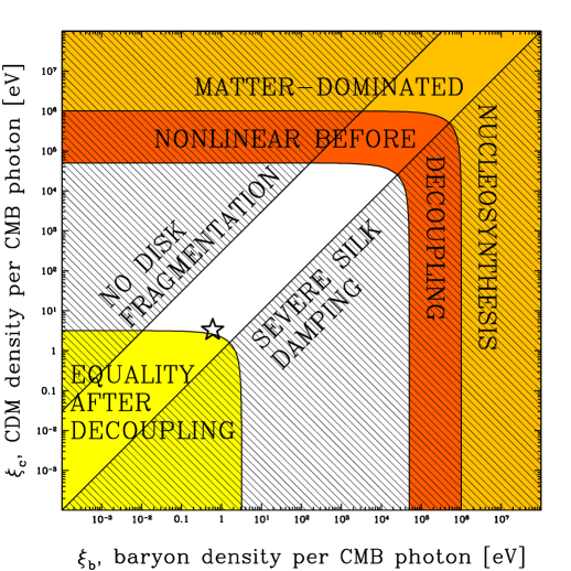
Figure 6: Qualitatively different parts of the $(\xi_{\rm b},\xi_{\rm c})$-plane. Our observed universe corresponds to the star, and altering the parameters to leave the white region corresponds to qualitative changes. The hatched regions delimit baryon fractions $fb=\xi_{\rm b}/\xi_{\rm c}>300$ and $fb<1$, which may suppress galaxy formation by impeding disk fragmentation and by Silk damping out Galaxy-scale matter clustering, respectively, The shaded regions delimit interesting ranges of constant total matter density parameter $\xi=\xi_{\rm b}+\xi_{\rm c}$ — to what extent these qualitative transitions are detrimental to galaxy formation deserves further work.

To conclude our discussion of selection effects, Figure 6 illustrates a number of constraints that are independent of $Q$ and $\rho_{\Lambda}$, depending on the density parameters $\xi_{\rm b}$ and $\xi_{\rm c}$ for baryonic and dark matter either through their ratio or their sum $\xi\equiv\xi_{\rm b}+\xi_{\rm c}$.

As we saw in Section III.2.2, a very low baryon fraction $f_{\rm b}\equiv\xi_{\rm b}/\xi\mathrel{\hbox to0.0pt{\lower 3.0pt\hbox{$\mathchar 536\relax$}\hss}\raise 2.0pt\hbox{$\mathchar 316\relax$}}300$ may preclude disk fragmentation and star formation. On the other hand, a baryon fraction of order unity corresponds to dramatically suppressed matter clustering on Galactic scales, since Silk damping around the recombination epoch suppresses fluctuations in the baryon component and the fluctuations that created the Milky Way were preserved through this epoch mainly by dark matter cmbfast .

Recombination occurs at $T\sim$Ry$/50\sim m_{\rm p}\alpha^{2}\beta/100\sim 3000{\rm K}$, whereas matter-domination occurs at ${T_{\rm eq}}\sim 0.2\xi$. If $\xi\mathrel{\hbox to0.0pt{\lower 3.0pt\hbox{$\mathchar 536\relax$}\hss}\raise 2.0pt\hbox{$\mathchar 316\relax$}}0.05m_{\rm p}\alpha^{2}\beta$, recombination would therefore precede matter-radiation equality, occurring during the radiation-dominated epoch. It is not obvious whether this would have detrimental effects on galaxy formation, but it is interesting to note that, as illustrated in Figure 6, our universe is quite close to this boundary in parameter space.

If we instead increase $\xi$, a there are two qualitative transitions.

In the limit $x=\rho_{\Lambda}/\rho_{\rm m}\ll 1$, using equation (15), equation (60) and $\rho_{\rm m}=\xi\ng$ gives

$$\sigma=\left({\pi^{2}\over 2\zeta(3)}\right)^{1/3}\sigma_{*}s(\mu){\xi Q\over T}\approx 0.33028\,s(\mu){\xi Q\over T}.$$ (49)

This means that the first Galactic mass structures ($s(\mu)\approx 28$) go nonlinear at $T\sim 9\xi Q$, i.e., before recombination if $\xi\mathrel{\hbox to0.0pt{\lower 3.0pt\hbox{$\mathchar 536\relax$}\hss}\raise 2.0pt\hbox{$\mathchar 318\relax$}}10^{-3}m_{\rm p}\alpha^{2}\beta m_{\rm p}/Q$. A baryonic cloud able to collapse before or shortly after recombination while the ionization fraction remained substantial would trap radiation and, as mentioned above in Section III.5, potentially produce a single black hole instead of stars.

Big Bang Nucleosynthesis (BBN) occurs at $T\sim m_{\rm p}\beta_{n}\sim 1\>{\rm MeV}$, so if we further increase $\xi$ so that $\xi\mathrel{\hbox to0.0pt{\lower 3.0pt\hbox{$\mathchar 536\relax$}\hss}\raise 2.0pt\hbox{$\mathchar 318\relax$}}m_{\rm p}\beta_{n}$, then the universe would be matter-dominated before BBN, producing dramatic (but not necessarily fatal Aguirre99 ) changes in primordial element abundances.

IV Putting it all together

As discussed in the introduction, theoretical predictions for physical parameters are confronted with observation using equation (1), where neither of the two factors $f_{\rm prior}({\bf p})$ and $f_{\rm selec}({\bf p})$ are optional. Above we discussed the two factors for the particular case study of cosmology and dark matter, covering the prior term in Section II and the selection effect term in Section III. Let us now combine the two and investigate the implications for the parameters $\xi$, $Q$ and $\rho_{\Lambda}$.

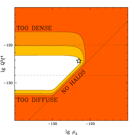
Figure 7: The fraction of all protons that end up in halos with density in the range $\rho_{\rm min}<\rho_{\rm vir}<\rho_{\rm max}$ is shown as a function of the cosmological parameters $\rho_{\Lambda}$ and $\rho_{*}\equiv Q^{3}\xi^{4}$. The contours show fractions $0.3$, $0.05$ and $0.003$ for the example $\rho_{\rm min}=10^{-128}$, $\rho_{\rm max}=10^{-120}$ (the two dashed lines) and $\mu=10^{-5}$ (corresponding roughly to $10^{12}M_{\odot}$ halos and giving $s(\mu)\approx 28$). When $\rho_{\Lambda}\gg Q^{3}\xi^{4}$, essentially no halos at all are formed. When $Q^{3}\xi^{4}\mathrel{\hbox to0.0pt{\lower 3.0pt\hbox{$\mathchar 536\relax$}\hss}\raise 2.0pt\hbox{$\mathchar 316\relax$}}10^{-3}\rho_{\rm min}$, essentially all halos have $\rho_{\rm vir}<\rho_{\rm min}$. When $Q^{3}\xi^{4}\mathrel{\hbox to0.0pt{\lower 3.0pt\hbox{$\mathchar 536\relax$}\hss}\raise 2.0pt\hbox{$\mathchar 318\relax$}}10^{2}\rho_{\rm max}$, essentially all halos have $\rho_{\rm vir}>\rho_{\rm max}$. The star shows our observed parameter values.

IV.1 An instructive approximation

For this exercise, we would ideally want to compute, say, the function $f_{\rm selec}({\bf p})$ defined as the fraction of protons ending up in stable habitable planets as function of $(\rho_{\Lambda},\xi,\xi_{\rm b},Q)$, leaving the particle physics parameters fixed at their observed values. Figure 3 shows that this is quite complicated, for two reasons. First, as discussed above we have computed only certain integrated versions of $f_{\rm selec}$. Second, the other selection effects discussed involve substantial uncertainties. To provide useful qualitative intuition, let us therefore start by working out the implications of the simple approximation that there are sharp upper and lower halo density cutoffs, i.e., that observers only form in halos within some density range $\rho_{\rm min}\leq\rho_{\rm vir}\leq\rho_{\rm max}$, where these two density limits may depend on $Q$, $\xi$ and $\xi_{\rm b}$. Based on the empirical observation that typical galaxies lie near the right side of the cooling curve in Figure 2, one would expect $\rho_{\rm min}$ to be determined by the bottom of the cooling curve and $\rho_{\rm max}$ by the intersection of the cooling curve with the encounter constraint.

Equation (20) showed that the fraction of all protons collapsing into a halo of mass $\mu$ is ${\mathrm{erfc}}[A(\rho_{\Lambda}/\rho_{*})^{1/3}/s(\mu){G_{\infty}}]$, where $\rho_{*}\equiv Q^{3}\xi^{4}$ can be crudely interpreted as the characteristic density of the first halos to form. Roughly, $A/s(\mu){G_{\infty}}\sim 1$, $\xi^{4}$ is the matter-radiation equality density and $Q^{3}$ is the factor by which our Universe gets diluted between equality (when fluctuations start to grow) and galaxy formation. More generally, of these protons, the fraction $f_{h}$ in halos within a density range $\rho_{\rm min}\leq\rho_{\rm vir}\leq\rho_{\rm max}$ is

$$f_{h}(\rho_{\Lambda},\xi,\xi_{\rm b},Q)={\mathrm{erfc}}\left[{(\rho_{\Lambda}/\hat{\rho}_{*})^{1/3}\over{G_{\Lambda}}(x(\rho_{\rm min}))}\right]-{\mathrm{erfc}}\left[{(\rho_{\Lambda}/\hat{\rho}_{*})^{1/3}\over{G_{\Lambda}}(x(\rho_{\rm max}))}\right],$$ (50)

where the function $x(\rho)$ is given by equation (24) extended so that $x(\rho)=\infty$ for $\rho\leq 16\rho_{\Lambda}$. For convenience, we have here defined the rescaled density

$$\hat{\rho}_{*}\equiv\left[{s(\mu)\over A}\right]^{3}\rho_{*}.$$ (51)

Figure 7 is a contour plot of this function, and illustrates that in addition to classical constraint $\rho_{\Lambda}\mathrel{\hbox to0.0pt{\lower 3.0pt\hbox{$\mathchar 536\relax$}\hss}\raise 2.0pt\hbox{$\mathchar 316\relax$}}Q^{3}\xi^{4}$ dating back to Weinberg and others BarrowTipler ; LindeLambda ; Weinberg87 ; Efstathiou95 ; Vilenkin95 ; Martel98 ; GarrigaVilenkin03 , we now have two new constraints as well: $\rho_{\Lambda}$-independent upper and lower bounds on $\rho_{*}\equiv Q^{3}\xi^{4}$.

IV.2 Marginalizing over $\rho_{\Lambda}$

As mentioned in Section II, there is good reason to expect the prior $f_{\rm prior}(\rho_{\Lambda},\xi,Q)$ to be independent of $\rho_{\Lambda}$ across the tiny relevant range $|\rho_{\Lambda}|\mathrel{\hbox to0.0pt{\lower 3.0pt\hbox{$\mathchar 536\relax$}\hss}\raise 2.0pt\hbox{$\mathchar 316\relax$}}Q^{3}\xi^{4}$ where $f_{\rm selec}(\rho_{\Lambda},\xi,Q)$ is non-negligible. This implies that we can write the predicted parameter probability distribution from equation (1) as

$$f(\rho_{\Lambda},\xi,\xi_{\rm b},Q)\propto f_{\rm prior}(\xi,\xi_{\rm b},Q)f_{o}(\xi,\xi_{\rm b},Q)f_{h}(\rho_{\Lambda},\xi,\xi_{\rm b},Q),$$ (52)

where $f_{o}(\xi,\xi_{\rm b},Q)$ is the product of all other selection effects that we have discussed — we saw that these were all independent of $\rho_{\Lambda}$.

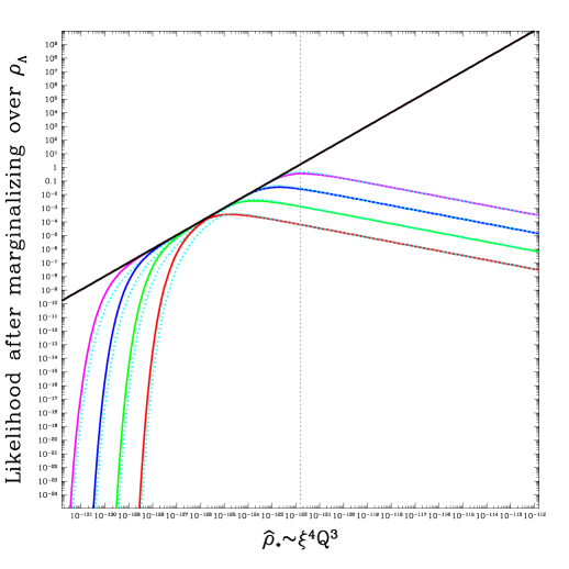
Figure 8: The probability factor $f_{h}(\rho_{*})$ after marginalizing over $\rho_{\Lambda}$. The black line of slope $1$ is for $\rho_{\rm min}=0$, $\rho_{\rm max}=\infty$. Increasing $\rho_{\rm min}$ shifts the exponential cutoff on the left side progressively further the right: $\rho_{\rm min}=10^{-5}$, $10^{-4}$, $10^{-3}$ and $10^{-2}$ times the density at the dotted horizontal line gives the four curves on the left. Decreasing $\rho_{\rm max}$ shifts left the break to a $-1/3$ slope further to the right: $\rho_{\rm max}=100$, $10$, $1$ and $0.1$ times the density at the dotted horizontal line gives the four downward-sloping curves on the right, respectively.

The key point here is that the only $\rho_{\Lambda}$-dependence in equation (52) comes from the $f_{h}$-term, i.e., from selection effects involving the halo banana. It is therefore interesting to marginalize over $\rho_{\Lambda}$ and study the resulting predictions for $Q$ and $\xi$. Thus integrating equation (52) over $\rho_{\Lambda}$, we obtain the theoretically predicted probability distribution

$$f(\xi,Q)\propto f_{\rm prior}(\xi,\xi_{\rm b},Q)f_{o}(\xi,\xi_{\rm b},Q)f_{h}(\xi,\xi_{\rm b},Q),\quad\hbox{where}$$

$$f_{h}(\xi,\xi_{\rm b},Q)\equiv\int_{0}^{\infty}f_{h}(\rho_{\Lambda},\xi,\xi_{\rm b},Q)d\rho_{\Lambda}.$$ (53)

Note that if $\rho_{\rm min}$ and $\rho_{\rm max}$ are constants, then $f_{h}(\xi,Q)$ is really a function of only one variable: since equation (50) shows that $\xi$ and $Q$ enter in $f_{h}(\rho_{\Lambda},\xi,Q)$ only in the combination $\rho_{*}\equiv Q^{3}\xi^{4}$, the marginalized result $f_{h}(\xi,Q)$ will be a function of $\rho_{*}$ alone. Figure 8 shows this function evaluated numerically for various values of $\rho_{\rm min}$ and $\rho_{\rm max}$, as well as the following approximation (dotted curves) which becomes quite accurate for $\rho\ll\rho_{\rm min}$ and $\rho\gg\rho_{\rm max}$:

$$f_{h}\approx\left\{724.9{\hat{\rho}_{*}^{1/3}\over\rho_{\rm max}^{4/3}}+{\sqrt{\pi}\over{G_{\infty}}^{3}\hat{\rho}_{*}{\mathrm{erfc}}\left[\left({\rho_{\rm min}\over 18\pi^{2}\hat{\rho}_{*}}\right)^{1/3}\right]}\right\}^{-1}$$ (54)

This approximation is valid also when $\rho_{\rm min}$ and $\rho_{\rm max}$ are functions of the cosmological parameters, as long as they are independent of $\rho_{\Lambda}$. To understand this result qualitatively, consider first the simple case where we count baryons in all halos regardless of density, i.e., $\rho_{\rm min}=0$, $\rho_{\rm max}=\infty$. Then a straightforward change of variables in equation (52) gives $f_{h}(\rho_{*})\propto\rho_{*}=Q^{3}\xi^{4}$, as was previously derived in inflation . This result troubled the authors of both inflation and GarrigaVilenkin05 , since any weak prior on $Q$ from inflation would be readily overpowered by the $Q^{3}$-factor, leading to the incorrect prediction of a much larger CMB fluctuation amplitude than observered. The same result would also spell doom for the axion dark matter model discussed in Section II.1, since the $\xi^{-1/2}$-prior would be overpowered by the $\xi^{4}$-factor from the selection effect and dramatically overpredict the dark matter abundance.

Figure 8 shows that the presence of selection effects on halo density has the potential to solve this problem. Both the problem and its potential resolution can be intuitively understood from Figure 7. Note that $f_{h}(\rho_{*})$ is simply the horizontal integral of this two-dimensional distribution. For $\rho_{\rm min}\ll\rho_{*}\ll\rho_{\rm max}$, the integrand $\approx 1$ out to the $\rho_{*}\sim\rho_{\Lambda}$-line marked “NO HALOS”, giving $f_{h}(\rho_{*})\propto\rho_{*}$. In the limit $\rho_{*}\gg\rho_{\rm max}$, however, we are integrating across the region marked ‘TOO DENSE” in Figure 8, and the result drops as $f_{h}(\rho_{*})\propto\rho_{\rm max}^{4/3}/\rho_{*}^{1/3}=\rho_{\rm max}^{4/3}/Q\xi^{4/3}$. This is why Figure 8 shows a break in slope from $+1$ to $-1/3$ at a location $\rho_{*}\sim\rho_{\rm max}/200$, as illustrated by the four curves with different $\rho_{\rm max}$-values. Conversely, in the limit $\rho_{*}\ll\rho_{\rm min}$, we are integrating across the exponentially suppressed region marked ‘TOO DIFFUSE” in Figure 7, causing a corresponding exponential suppression in Figure 7 for $\rho_{*}\ll\rho_{\rm min}$.

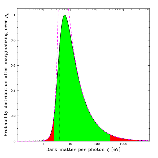
Figure 9: Probability distribution for the axion dark matter density parameter $\xi$ measured from a random $10^{12}M_{\odot}$ halo with virial density below 5000 times the present cosmic matter density. Green/light shading indicates the 95% confidence interval. The dotted vertical line shows our observed value $\xi\approx 4$ eV, in good agreement with the prediction. The dashed curves show the analytic asymptotics $\xi^{9/2}$ and $\xi^{-5/6}$, respectively.

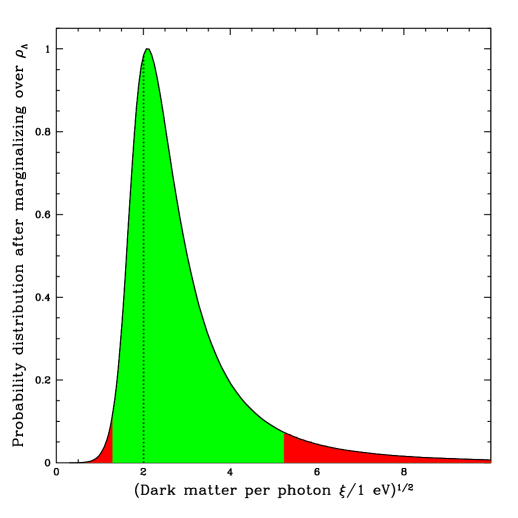
Figure 10: Same as previous figure, but showing the probability distribution for $\xi^{1/2}$, the quantity which has a uniform prior in our axion model. The shape of this curve therefore reflects the selection effect alone.

Figures 9 and 10 illustrate this for the simple example of using the Section II.1 axion prior $f_{\rm prior}(\xi)\propto\xi^{-1/2}$, treating $Q$ as fixed at its observed value, ignoring additional selection effects ($f_{o}(\xi)=1$), and imposing a halo density cutoff $\rho_{\rm max}$ of 5000 times the current cosmic matter density.

The key features of this plot follow directly from our analytic approximation of equation (54). First, for $\rho_{*}\ll\rho_{\rm max}$, we saw that $f_{h}\propto\rho_{*}\propto\xi^{4}$, so equation (IV.2) gives the probability growing as $f\propto\xi^{-1/2}\xi^{4}\xi=\xi^{9/2}$ (the last $\xi$-factor comes from the fact that we are plotting the probability distribution for $\log\xi$ rather than $\xi$). This means that imposing a lower density cutoff $\rho_{\rm min}$ would have essentially no effect. This also justifies our approximation of using the total matter density parameter $\xi$ as a proxy for the dark matter density parameter $\xi_{\rm c}$: we have a baryon fraction $\xi_{\rm b}/\xi_{\rm c}\ll 1$ in the interesting regime, with a negligible probability for $\xi_{\rm c}\mathrel{\hbox to0.0pt{\lower 3.0pt\hbox{$\mathchar 536\relax$}\hss}\raise 2.0pt\hbox{$\mathchar 316\relax$}}\xi_{\rm b}\sim 0.6{\rm eV}$ (the probability curve continues to drop still further to the left even without the $f_{h}$-factor). Second, for $\rho_{*}\gg\rho_{\rm max}$, we saw that $f_{h}\propto\rho_{*}^{-1/3}\propto\xi^{-4/3}$, so equation (IV.2) gives the probability falling as $f(\ln\xi)\propto\xi^{-1/2}\xi^{-4/3}\xi=\xi^{-5/6}$.

Although this simple example was helpful for building intuition, a more accurate treatment is required before definitive conclusions about the viability of the axion dark matter model can be drawn. One important issue, to which we return below in Section IV, is the effect of the unknown $Q$-prior, since the preceding equations only constrained a combination of $Q$ and $\xi$. A second important issue, to which we devote the remainder of this subsection, has to do with properly incorporating the constraints from Figure 3. If we only consider the encounter constraint and make the unphysical simplification of ignoring the effect of halo velocity dispersion, then our upper limit should be not on dark matter density ($\rho_{\rm max}$ constant) but on baryon density ($\rho_{\rm max}\xi_{\rm b}/\xi$ constant). Inserting this into equation (54) makes the term $\hat{\rho}_{*}^{1/3}/\rho_{\rm max}^{4/3}$ independent of $\xi$ as $\xi\to\infty$, replacing the $f_{h}\propto Q^{-1}\xi^{-4/3}$ cutoff by $f_{h}\propto Q^{-1}\xi_{\rm b}^{-4/3}$, which is constant if $\xi_{\rm b}$ is. The axion prior would then predict a curve $f(\ln\xi)\propto\xi^{1/2}$ rising without bound. This failure, however, results from ignoring some of the physics from Figure 3. Considering a series of nominally more likely domains with progressively larger $\xi$, they typically have more dark energy ($\rho_{\Lambda}\propto\xi$) and higher characteristic halo baryon density ($n_{\rm vir}\propto\xi^{3}\xi_{\rm b}$), so stable solar systems are found only in rare galaxies that formed exceptionally late, just before $\rho_{\Lambda}$-domination, with $n_{\rm vir}\propto\rho_{\rm vir}\xi_{\rm b}/\xi\mathrel{\hbox to0.0pt{\lower 3.0pt\hbox{$\mathchar 536\relax$}\hss}\raise 2.0pt\hbox{$\mathchar 318\relax$}}16\rho_{\Lambda}\xi_{\rm b}/\xi\propto\xi_{\rm b}$ roughly $\xi$-independent and below the the maximum allowed value. Since the increased dark matter density boosts virial velocities, this failure mode corresponds to moving from the star in Figure 3 straight to the right, running right into the constraints from cooling and velocity-dependent encounters. In other words, a more careful calculation would be expected to give a prediction qualitatively similar to that of Figure 9. The lower cutoff would remain visually identical to that of Figure 9 as long as $\rho_{\rm min}$ can be neglected in the calculation, whereas the upper cutoff would become either steeper or shallower depending on the details of the encounter and cooling constraints. This interesting issue merits further work going well beyond the scope of the present paper, extending our treatment of halo formation, halo mergers and galaxy formation into a quantitative probability distribution in the plane of Figure 3, i.e., into a function $f(T_{\rm vir},n_{\rm vir};Q,\rho_{\Lambda},\xi,\xi_{\rm b})$ that could be multiplied by the plotted constraints and marginalized over $(T_{\rm vir},n_{\rm vir})$ to give $f_{\rm selec}(Q,\rho_{\Lambda},\xi,\xi_{\rm b})$.

IV.3 Predictions for $\rho_{\Lambda}$

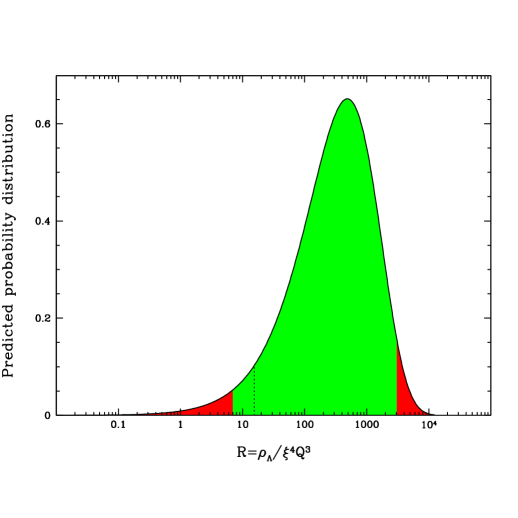
Figure 11: Probability distribution for the quantity $R\equiv\rho_{\Lambda}/\xi^{4}Q^{3}$ measured from a random $10^{12}M_{\odot}$ halo, using a uniform prior for $R$ and ignoring other selection effects. This is equivalent to treating $\xi$ and $Q$ as fixed. Green/light shading indicates the 95% confidence interval, the dotted line indicates the observed value $R\approx 15$.

This above results also have important implications for the dark energy density $\rho_{\Lambda}$. The most common way to predict its probability distribution in the literature has been to treat all other parameters as fixed and assume both that the number of observers is proportional to the matter fraction in halos (which in our notation means $f_{\rm selec}(p)={\mathrm{erfc}}[A(\rho_{\Lambda}/Q^{3}\xi^{4})^{1/3}/s(\mu){G_{\infty}}]$) and that $f_{\rm prior}(\rho_{\Lambda})$ is constant across the narrow range $|\rho_{\Lambda}|\mathrel{\hbox to0.0pt{\lower 3.0pt\hbox{$\mathchar 536\relax$}\hss}\raise 2.0pt\hbox{$\mathchar 316\relax$}}Q^{3}\xi^{4}$ where $f_{\rm selec}$ is non-negligible. This gives the familiar result shown in Figure 11: a probability distribution consistent with the observed $\rho_{\Lambda}$-value but favoring slightly larger values. The numerical origin of the predicted magnitude $\rho_{\Lambda}\sim 10^{-123}$ is thus the measured value of $\rho_{*}\equiv Q^{3}\xi^{4}$.

Generalizing this to the case where $Q$ and/or $\xi$ can vary across an inflationary multiverse, the predictions will depend on the precise question asked. Figure 11 then shows the successful prediction for $\rho_{\Lambda}$ given (conditionalized on) our measured values for $Q$ and $\xi$. However, when testing a theory, we wish to use all opportunities that we have to potentially falsify it, and each predicted parameter offers one such opportunity. For our axion example, the theory predicts a 2-dimensional distribution in the $(\rho_{\Lambda},\xi)$-plane of which Figure 9 is the marginal distribution for $\xi$. The corresponding marginal distribution for $\rho_{\Lambda}$ (marginalized over $\xi$) will generally differ from Figure 11 in both its shape and in the location of its peak. It will differ in shape because the $(\rho_{\Lambda},\xi)$-distribution is not generally separable: the selection effects (as in Figure 11) will not be a function of $\rho_{\Lambda}$ times a function of $\xi$; in other words, a uniform prior on $\rho_{\Lambda}$ will not correspond to a uniform prior on the quantity $R\equiv\rho_{\Lambda}/Q^{3}\xi^{4}$ plotted in Figure 7 once non-separable selection effects such as ones on the halo density parameter $\rho_{*}\equiv Q^{3}\xi^{4}$ are included. Moreover, the distribution will in general not peak where that in Figure 11 does because the predicted magnitude $\rho_{\Lambda}\sim 10^{-123}$ no longer comes from conditioning on astrophysical measurements of $Q$ and $\xi$, but from other parameters like $\alpha$, $\beta$ and $m_{\rm p}$ that determine the selection effects in Figure 3 and the maximum halo density $\rho_{\rm max}$. In this case, whether the observed $\rho_{\Lambda}$-value agrees with predictions or not thus depends sensitively on how strong the selection effects against dense halos are.

In summary, the prediction of $\rho_{\Lambda}$ given $Q$ and $\xi$ is an unequivocal success, whereas predictions for $Q$, $\xi$ and the entire joint distribution for $(\rho_{\Lambda},\xi,Q)$ are fraught with the above-mentioned uncertainties. Since a uniform $\rho_{\Lambda}$-prior does not imply a uniform $R\equiv\rho_{\Lambda}/Q^{3}\xi^{4}$-prior, we cannot conclude that anthropic arguments succeed in predicting $R\equiv\rho_{\Lambda}/Q^{3}\xi^{4}$ GarrigaVilenkin05 without additional hypotheses.

IV.4 Constraint summary

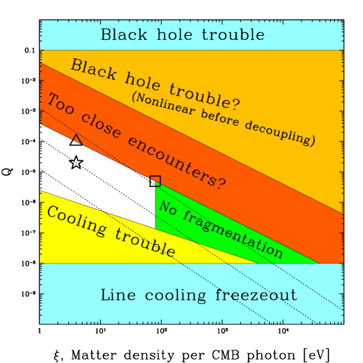
Figure 12: Crude summary of constraints $(\xi,Q)$-plane constraints from Table 4. The star shows our observation $(\xi,Q)\approx(4{\rm eV},2\times 10^{-5})$. The parallel dotted lines are lines of constant characteristic halo density, so the constraint that dark matter halos form (that they go nonlinear before vacuum domination freezes fluctuation growth) rules out everything to the lower left of these lines, which from left to right correspond to $\rho_{\Lambda}/\rho_{\Lambda}^{\rm obs}=10^{-3}$, $1$, $10^{3}$. This means that if $\xi$ is fixed, marginalizing over $\rho_{\Lambda}$ pushes things to the triangle at larger $Q$ (the “smoothness problem” inflation ), but if $\xi$ too can vary, marginalizing over $\rho_{\Lambda}$ instead pushes things to the square at smaller $Q$.

Table 4: These constraints (see text) are summarized in Figure 12

Constraint	Generally	Fixing $(\alpha,\beta,m_{\rm p})$	Fixing all but $(Q,\xi)$
Need nonlinear halos	$|\rho_{\Lambda}|\mathrel{\hbox to0.0pt{\lower 3.0pt\hbox{$\mathchar 536\relax$}\hss}\raise 2.0pt\hbox{$\mathchar 316\relax$}}\rho_{*}$	$|\rho_{\Lambda}|/\xi^{4}Q^{3}\mathrel{\hbox to0.0pt{\lower 3.0pt\hbox{$\mathchar 536\relax$}\hss}\raise 2.0pt\hbox{$\mathchar 316\relax$}}1$	$Q\mathrel{\hbox to0.0pt{\lower 3.0pt\hbox{$\mathchar 536\relax$}\hss}\raise 2.0pt\hbox{$\mathchar 318\relax$}}10^{-5}(\xi/\xi_{0})^{-4/3}$
Avoid line cooling freezeout	$Q\mathrel{\hbox to0.0pt{\lower 3.0pt\hbox{$\mathchar 536\relax$}\hss}\raise 2.0pt\hbox{$\mathchar 318\relax$}}\alpha^{2}\beta$	$Q\mathrel{\hbox to0.0pt{\lower 3.0pt\hbox{$\mathchar 536\relax$}\hss}\raise 2.0pt\hbox{$\mathchar 318\relax$}}10^{-8}$	$Q\mathrel{\hbox to0.0pt{\lower 3.0pt\hbox{$\mathchar 536\relax$}\hss}\raise 2.0pt\hbox{$\mathchar 318\relax$}}10^{-8}$
Primordial black hole excess	$Q\mathrel{\hbox to0.0pt{\lower 3.0pt\hbox{$\mathchar 536\relax$}\hss}\raise 2.0pt\hbox{$\mathchar 316\relax$}}10^{-1}$	$Q\mathrel{\hbox to0.0pt{\lower 3.0pt\hbox{$\mathchar 536\relax$}\hss}\raise 2.0pt\hbox{$\mathchar 316\relax$}}10^{-1}$	$Q\mathrel{\hbox to0.0pt{\lower 3.0pt\hbox{$\mathchar 536\relax$}\hss}\raise 2.0pt\hbox{$\mathchar 316\relax$}}10^{-1}$
Need cooling in Hubble time	$Q^{3}\xi_{\rm b}^{2}\xi^{2}\mathrel{\hbox to0.0pt{\lower 3.0pt\hbox{$\mathchar 536\relax$}\hss}\raise 2.0pt\hbox{$\mathchar 318\relax$}}\alpha^{-3}\ln[\alpha^{-2}]^{-16/3}\beta^{4}m_{\rm p}^{6}/125$	$Q^{3}\xi_{\rm b}^{2}\xi^{2}\mathrel{\hbox to0.0pt{\lower 3.0pt\hbox{$\mathchar 536\relax$}\hss}\raise 2.0pt\hbox{$\mathchar 318\relax$}}10^{-129}$	$Q\mathrel{\hbox to0.0pt{\lower 3.0pt\hbox{$\mathchar 536\relax$}\hss}\raise 2.0pt\hbox{$\mathchar 318\relax$}}10^{-6}(\xi/\xi_{0})^{-2/3}$
Avoid close encounters		$Q^{3}\xi_{\rm b}\xi^{3}\mathrel{\hbox to0.0pt{\lower 3.0pt\hbox{$\mathchar 536\relax$}\hss}\raise 2.0pt\hbox{$\mathchar 316\relax$}}10^{-123}$	$Q\mathrel{\hbox to0.0pt{\lower 3.0pt\hbox{$\mathchar 536\relax$}\hss}\raise 2.0pt\hbox{$\mathchar 316\relax$}}10^{-4}(\xi/\xi_{0})^{-1}$
Go nonlinear after decoupling	$\xi Q\mathrel{\hbox to0.0pt{\lower 3.0pt\hbox{$\mathchar 536\relax$}\hss}\raise 2.0pt\hbox{$\mathchar 316\relax$}}10^{-3}\alpha^{2}\beta m_{\rm p}$	$\xi Q\mathrel{\hbox to0.0pt{\lower 3.0pt\hbox{$\mathchar 536\relax$}\hss}\raise 2.0pt\hbox{$\mathchar 316\relax$}}10^{-30}$	$Q\mathrel{\hbox to0.0pt{\lower 3.0pt\hbox{$\mathchar 536\relax$}\hss}\raise 2.0pt\hbox{$\mathchar 316\relax$}}10^{-2}(\xi/\xi_{0})^{-1}$
Need equality before decoupling?	$\xi\mathrel{\hbox to0.0pt{\lower 3.0pt\hbox{$\mathchar 536\relax$}\hss}\raise 2.0pt\hbox{$\mathchar 318\relax$}}0.05\alpha^{2}\beta m_{\rm p}$	$\xi\mathrel{\hbox to0.0pt{\lower 3.0pt\hbox{$\mathchar 536\relax$}\hss}\raise 2.0pt\hbox{$\mathchar 318\relax$}}10^{-28}$	$(\xi/\xi_{0})\mathrel{\hbox to0.0pt{\lower 3.0pt\hbox{$\mathchar 536\relax$}\hss}\raise 2.0pt\hbox{$\mathchar 318\relax$}}1/3$
Avoid severe Silk damping	$f_{\rm b}\mathrel{\hbox to0.0pt{\lower 3.0pt\hbox{$\mathchar 536\relax$}\hss}\raise 2.0pt\hbox{$\mathchar 316\relax$}}1/2$	$\xi/\xi_{\rm b}\mathrel{\hbox to0.0pt{\lower 3.0pt\hbox{$\mathchar 536\relax$}\hss}\raise 2.0pt\hbox{$\mathchar 318\relax$}}2$	$(\xi/\xi_{0})\mathrel{\hbox to0.0pt{\lower 3.0pt\hbox{$\mathchar 536\relax$}\hss}\raise 2.0pt\hbox{$\mathchar 318\relax$}}1/3$
Need disk instability	$f_{\rm b}\mathrel{\hbox to0.0pt{\lower 3.0pt\hbox{$\mathchar 536\relax$}\hss}\raise 2.0pt\hbox{$\mathchar 316\relax$}}10^{2}$	$\xi_{\rm c}/\xi_{\rm b}\mathrel{\hbox to0.0pt{\lower 3.0pt\hbox{$\mathchar 536\relax$}\hss}\raise 2.0pt\hbox{$\mathchar 316\relax$}}10^{2}$	$(\xi/\xi_{0})\mathrel{\hbox to0.0pt{\lower 3.0pt\hbox{$\mathchar 536\relax$}\hss}\raise 2.0pt\hbox{$\mathchar 316\relax$}}20$

Table 4 summarizes the constraints that we have discussed above. Those not superseded by other stronger ones are also illustrated in Figure 12, with $\xi_{\rm b}$ fixed at its observed value. Let us briefly comment on how they all fit together.

The first key point to note in Figure 12 is that the various constraints involve many different combinations of $Q$ and $\xi$, thereby breaking each other’s degeneracies and providing interesting constraints on both $\xi$ and $Q$ separately. The fragmentation constraint (requiring disk instability) constrains $\xi$ alone when $\xi_{\rm b}$ is given whereas there are constraints on $Q$ alone from both line cooling freezeout and primordial black hole trouble. The encounter and cooling constraints both have different slopes ($-1$ and $-2/3$, respectively) because they involve different powers of the baryon fraction. Whereas the nonlinear halo constraint depends on the total halo density $\propto Q^{3}\xi^{4}$, the encounter constraint depends on the halo baryon density $\propto Q^{3}\xi^{3}\xi_{\rm b}$. The cooling constraint (which is equation (11) in Q after changing variables to reflect the notation in this paper) comes from equating the cooling timescale (given by the inverse of the baryon density $\propto Q^{3}\xi^{3}\xi_{\rm b}$) and the dynamical timescale (given by the total density as $\propto\rho_{\rm vir}^{-1/2}\propto(Q^{3}\xi^{4})^{-1/2}$, thus constraining the combination $Q^{3}\xi^{2}\xi_{\rm b}^{2}$.

The second key point in Figure 12 is that this combination of constraints reverses previously published conclusions about $Q$. Where we should expect to find ourselves in Figure 12 depends on the priors for both $Q$ and $\xi$. Recall that halos form only above whichever dotted line corresponds to the $\rho_{\Lambda}$-value. If the prior for $\rho_{\Lambda}$ is indeed uniform, then it is a priori (before selection effects are taken into account) 1000 times more likely for the halo constraint to be the upper dotted line than the middle one, and this is in turn 1000 more likely than the bottom dotted line. In other words, marginalizing over $\rho_{\Lambda}$ relentlessly pushes us towards the upper right in Figure 12, towards larger value of $\rho_{*}=Q^{3}\xi^{4}$. This means that if $\xi$ is fixed and only $Q$ can vary across the ensemble, marginalizing over $\rho_{\Lambda}$ pushes things towards the triangle at larger $Q$. This “smoothness problem” was pointed out in Q and elaborated in Garriga99 ; Graesser04 ; inflation , suggesting that unless the $f_{\rm prior}(Q)$ falls off as $Q^{-4}$ or faster, it is overpowered by the selection effect and one predicts a clumpier universe than observed (the star in Figure 12 should be shifted vertically up against the edge of the encounter constraint, to the triangle). Figure 12 shows that if $\xi$ too can vary, marginalizing over $\rho_{\Lambda}$ instead pushes things towards smaller $Q$, to the square, since this gives the greatest allowed halo density $\propto Q^{3}\xi^{4}$. In inflation , it was found that certain low-energy inflation scenarios naturally predicted a rather flat priors for $\lg Q$ — to determine whether they are ruled out or not thus requires more detailed modeling of the effect of the dark matter density on galaxy formation and encounters.

Table 4 illustrates that (except for one rather unimportant logarithm), all constraints we have considered correspond to hyperplanes in the 7-dimensional space parametrized by

$$(\lg\alpha,\lg\beta,\lg m_{\rm p},\lg\rho_{\Lambda},\lg Q,\lg\xi,\lg\xi_{\rm b}),$$ (55)

providing a simple geometric interpretation of the selection effects. This means that if all priors are power laws, the preferred parameter values are determined by solving a simple linear programming problem, and will generically correspond to one of the corners of the convex 7-dimensional allowed region. Above we have frequently used such sharp inequalities to help build intuition for the underlying physics. For future extensions of this work, however, it should be borne in mind that such inequalities are not necessarily sufficient to capture the key features of the problem, and that they can either overstate or understate the importance of selection effects. The ultimate goal is to test theories by computing the predicted probability distribution from equation (1), and almost no selection effects $f_{\rm selec}({\bf p})$ correspond to sharp cutoffs resembling a Heaviside step function. Some (like the halo constraint) are exponential and thus able to overpower any power law prior. Others, however, may be softer, and it is therefore crucial to check whether their functional form falls of faster than than the relevant prior grows — if not, the “constraint” will be penetrated, and the most likely parameter values may lie in the allegedly “disallowed region”. Conversely, if $f({\bf p})=f_{\rm prior}({\bf p})f_{\rm selec}({\bf p})$ is rather flat in a large “allowed region”, then the most likely parameter values can lie well inside it, far from any edges, since it corresponds to the peak of the probability distribution rather than its edge.

V Conclusions

We have discussed predictions for the 31-dimensional vector ${\bf p}$ of dimensionless physical constants in the context of “ensemble theories” producing multiple Hubble volumes (“universes”) between which one or more of the parameters can differ. The prediction is the probability distribution of equation (1), where neither of the two factors is optional. Although it is generally difficult to evaluate either one of the terms, it is nonetheless crucial: if candidate theories involve such ensembles, they are neither testable nor falsifiable unless their probabilistic predictions can be computed.

Although many scientists hope that $f_{\rm prior}$ in equation (1) will be a multidimensional Dirac $\delta$-function, rendering selection effects irrelevant, to elevate this hope into an assumption would, ironically, be to push the anthropic principle to a hedonistic extreme, suggesting that nature must be devised so as to make mathematical physicists happy. We must therefore face some difficult questions both about what, in principle, to select on, and how to quantitatively calculate that selection effect. For both statistical mechanics and quantum mechanics, it proved challenging to correctly predict probability distributions. If the analogous challenge can be overcome for theories predicting dimensionless constants, they too will become testable in the same fashion. The fact that we can only observe once is not a show-stopper: a single observation of a vertically polarized photon passing through a polarizer $\theta=89.9^{\circ}$ from vertical would rule out quantum mechanics at $1-\cos^{2}\theta\approx 99.9997\%$ confidence. The outstanding difficulty is therefore not a “philosophical” problem that we cannot observe the full ensemble, but rather that we generally do not know how to compute the theoretical prediction $f({\bf p})$.

V.1 Axion dark matter

We have tackled this problem quantitatively for a particular example where both factors in equation (1) are computable: that of axion dark matter with its phase transition well before the end of inflation. We found that $f_{\rm prior}(\xi)\propto\xi^{-1/2}$, i.e., that the prior dark matter distribution has no free parameters even though the axion model itself does. We saw that this useful predictability gain has the same basic origin as that of the zero-parameter (flat) $\rho_{\Lambda}$-prior of Weinberg87 : the anthropically relevant range over which $f_{\rm selec}$ is non-negligible is much smaller than the natural range of $f_{\rm prior}$, so only a particular property of $f_{\rm prior}$ matters. For the famous $\rho_{\Lambda}$-case, the natural $f_{\rm prior}$-range involves either the supersymmetry-breaking scale or the Planck scale $|\rho_{\Lambda}|\mathrel{\hbox to0.0pt{\lower 3.0pt\hbox{$\mathchar 536\relax$}\hss}\raise 2.0pt\hbox{$\mathchar 316\relax$}}\rho_{\rm planck}$ whereas the relevant range is $|\rho_{\Lambda}|\mathrel{\hbox to0.0pt{\lower 3.0pt\hbox{$\mathchar 536\relax$}\hss}\raise 2.0pt\hbox{$\mathchar 316\relax$}}10^{-123}\rho_{\rm planck}$, so the property that $f_{\rm prior}(\rho_{\Lambda})$ is smooth on that tiny scale implies that it is for all practical purposes constant. For our $\xi$-case, the natural $f_{\rm prior}$-range is $0\leq\xi\leq\xi_{*}$ where $\xi_{*}^{1/4}$ lies somewhere between the inflation scale and the Planck scale, whereas the relevant range is much smaller, so the only property of $f_{\rm prior}(\xi)$ that matters is its asymptotic scaling as $\xi\to 0$.

In computing the selection effect factor $f_{\rm selec}(\rho_{\Lambda},\xi,Q)$, we took advantage of the fact that none of these parameters affect chemistry or biology directly. We could therefore avoid poorly understood biochemical issues related to life and consciousness, and could limit our calculations to astrophysical selection effects involving halo formation, galaxy, solar system stability, etc. The same simplifying argument has been previously applied to $\rho_{\Lambda}$ and the neutrino density (e.g., anthrolambdanu ). We discovered that combining various astrophysical selection effects with all three parameters $(\rho_{\Lambda},Q,\xi)$ as variables reversed previous conclusions (Figure 12), pushing towards lower rather than higher $Q$-values. In particular, we found that one can reach misleading conclusions by simply taking $f_{\rm selec}$ to be the matter fraction collapsing into halos, neglecting the fact that very dense halos limit planetary stability. In particular, we found that if we impose a stiff upper limit on the density of habitable halos, the predicted probability distribution for the dark matter density parameter (Figure 9) can be brought into agreement with the measured $\xi$-value for reasonable assumptions, i.e., that the pre-inflationary axion model is a viable dark matter theory.

V.2 Multiple dark matter components

Suppose that supersymmetry were to be discovered at the Large Hadron Collider, indicating the existence of a weakly interacting massive particle (WIMP) with a relic density approximately equal to the observed dark matter density, i.e., with $\xi_{\rm wimp}\sim\xi_{\rm c}$. There would then be a strong temptation to declare the dark matter problem solved. Based on our results, however, that would be quite premature!

As detailed in Section II.2, it is not implausible that the function $f_{\rm prior}(\xi_{\rm wimp})$ to be taken as input to the astrophysics calculation is a sharply peaked function whose relative width is much narrower than that of $f_{\rm selec}(\xi_{\rm c})$, perhaps only a few percent. This situation could arise if the fundamental theory predicted a broad prior only for the $\mu^{2}$-parameter in Table 1 (which controls the Higgs vacuum expectation value), since this may arguably be determined to within a few percent from selection effects in the nuclear physics sector, notably stellar carbon and oxygen production. If the pre-inflationary axion model is correct, we would then have

$$\xi_{\rm c}=\xi_{\rm wimp}+\xi_{\rm axion},$$ (56)

where $f_{\rm prior}(\xi_{\rm axion})\propto\xi_{\rm axion}^{-1/2}$ and $\xi_{\rm wimp}$ would be for all practical purposes a constant. This gives $f_{\rm prior}(\xi_{\rm c})\propto(\xi_{\rm c}-\xi_{\rm wimp})^{-1/2}$ for $\xi_{\rm c}\geq\xi_{\rm wimp}$, zero otherwise, and the testable prediction becomes this times the astrophysical factor selection effects factor $f_{\rm selec}(\xi_{\rm c})$ that we have discussed. Repeating the calculation of conditionalization , this implies that we should expect to find roughly comparable densities of WIMP and axion dark matter.

As shown in conditionalization , removing the assumption that $f_{\rm prior}(\xi_{\rm wimp})$ is sharply peaked does not alter this qualitative conclusion. This conclusion would also hold for any other axion-like fields that were energetically irrelevant during inflation, even unrelated to the strong CP-problem. More generally, string-inspired model building suggests the possibility that multiple species of “GIMPS” (gravitationally interacting massive particles that do not couple through the electromagnetic, weak or strong interactions) may be present. According to recent understanding, their presence may be expected for modular inflation, though not for brane inflation DouglasPC . If such particles exist and have generic not-too-extreme priors (falling no faster than $\xi^{-1}$ and rising no faster than the selection effect cutoff), then our anthropic constraints on the sum of their densities again predict a comparable density for all of species of dark matter that have a rising prior conditionalization .

Even before the LHC turns on, more careful calculation of the astrophysical selection effects determining $f_{\rm selec}$ could give interesting hints. If the constraints on dense halos turn out to be rather weak so that the improved version of Figure 9 predicts substantially more axion dark matter than observed, this will favor an alternative model such as WIMPs where $f_{\rm prior}(\xi_{\rm c})$ is so narrow that $\xi_{\rm c}$ is effectively determined non-anthropically. Alternatively, if Figure 9 remains consistent with observation, then it will be crucial to follow up an initial LHC SUSY or other WIMP detection, if it occurs, with detailed measurements of the relevant parameters to establish whether the WIMP density accounted for (which a linear collider might, in favorable cases, pinpoint within a few percent Feng05 ) is exactly equal to the cosmologically measured dark matter density, or whether a substantial fraction of the dark matter still remains to be accounted for.

The authors wish to thank Ed Bertschinger, Douglas Finkbeiner, Alan Guth, Craig Hogan, Andrei Linde and Matias Steinmetz for helpful comments, and Sam Ribnick for some earlier, exploratory calculations. Thanks to Tom Abel for molecular cooling software. This work was supported by NASA grant NAG5-11099, NSF CAREER grant AST-0134999, and fellowships from the David and Lucile Packard Foundation and the Research Corporation. The work of AA was supported in part by NSF grant AST-0507117. The work of FW is supported in part by funds provided by the U.S. Department of Energy under cooperative research agreement DE-FC02-94ER40818.

Appendix A Fitting functions used

In this Appendix, we derive a variety of fitting functions used in the paper, explicitly highlighting the dependence of standard cosmological structure formation on the dimensionless parameters $\xi$, $\rho_{\Lambda}$, $Q$ and $\mu$. Since some of our approximations are quite accurate, we retain the exact numerical coefficients where appropriate.

A.1 The fluctuation time dependence $G(x)$

As shown in anthroneutrino , the function

$${G_{\Lambda}}(x)\approx x^{1/3}\left[1+\left({x\over{G_{\infty}}^{3}}\right)^{\alpha}\right]^{-1/3\alpha},$$ (57)

where $\alpha=159/200=0.795$ and

$${G_{\infty}}\equiv{5\Gamma\left({2\over 3}\right)\Gamma\left({5\over 6}\right)\over 3\sqrt{\pi}}\approx 1.43728,$$ (58)

describes how, in the absence of massive neutrinos, fluctuations in a $\rho_{\Lambda}>0$ $\Lambda$CDM universe grow as the cosmic scale factor $a$ as long as dark energy is negligible (${G_{\Lambda}}(x)\approx x^{1/3}\propto a\propto(1+z)^{-1}$ for $x\ll 1$) and then asymptote to a constant value as $t\to\infty$ and dark energy dominates (${G_{\Lambda}}(x)\to{G_{\infty}}$ as $x\to\infty$).

Including the effect of radiation domination early on but ignoring baryon-photon coupling, the total growth factor is well approximated by anthroneutrino

$$G(x)\approx 1+{3\over 2}x_{\rm eq}^{-1/3}{G_{\Lambda}}(x),$$ (59)

which is accurate to better than 1.5% for all $x$ anthroneutrino . In essence, fluctuations grow as $\delta\propto a\propto x^{1/3}$ between matter domination ($x=x_{\rm eq}$) and dark energy domination ($x=1$), giving a net growth of $x_{\rm eq}^{-1/3}$. Equation (59) shows that they grow by an extra factor of 1.5 by starting slightly before matter domination and by an extra factor ${G_{\Lambda}}(\infty)\approx 1.44$ by continuing to grow slightly after dark energy domination.

Let us now simplify this result further. From the definition of $\xi$, the matter density can be written $\rho_{\rm m}=\xi\ng$, where $\ng$ is the number density of photons. The latter is given (in Planck units) by the standard black body formula

$$\ng={2\zeta(3)\over\pi^{2}}T^{3},\quad\zeta(3)\approx 1.20206.$$ (60)

The corresponding standard formula for the energy density is

$$\rho_{\gamma}={\pi^{2}\over 15}T^{4}$$ (61)

for photons and

$$\rho_{\nu}^{\gamma}={21\over 8}\left({4\over 11}\right)^{4/3}\rho_{\gamma}\approx 0.68132\rho_{\gamma}$$ (62)

for three standard species of relativistic massless neutrinos. The matter-radiation equality temperature where $\rho_{\rm m}=\rho_{\gamma}+\rho_{\nu}^{\gamma}$ is thus

$${T_{\rm eq}}={30\zeta(3)\over\pi^{4}}{\left[1+{21\over 8}\left({4\over 11}\right)^{4/3}\right]^{-1}}\xi\approx 0.220189\xi,$$ (63)

measured to be about $9400{\rm K}$ in our Hubble volume. Since $x_{\rm eq}=\rho_{\Lambda}/\rho_{\rm m}^{\rm eq}=\rho_{\Lambda}/\xi\ng({T_{\rm eq}})$, we thus obtain

$$x_{\rm eq}={\pi^{14}\over 2\cdot 30^{3}\zeta(3)^{4}}\left[1+{21\over 8}\left({4\over 11}\right)^{4/3}\right]^{3}{\rho_{\Lambda}\over\xi^{4}}\approx 384.554{\rho_{\Lambda}\over\xi^{4}}$$ (64)

The above relations are summarized in Tables 2 and 3. In all cases of relevance to the present paper, the growth factor $G(x)\gg 1$, allowing initial fluctuations $Q\ll 1$ to grow enough to go nonlinear. We can therefore drop the first term in equation (59), obtaining the useful result

$$G(x) \approx {45\cdot 2^{1/3}\zeta(3)^{4/3}\over\pi^{14/3}}\left[1+{21\over 8}\left({4\over 11}\right)^{4/3}\right]^{-1}{\xi^{4/3}\over\rho_{\Lambda}^{1/3}}{G_{\Lambda}}(x)$$ (65)

$$\approx 0.206271{\xi^{4/3}\over\rho_{\Lambda}^{1/3}}{G_{\Lambda}}(x).$$

A.2 The fluctuation scale dependence $s(\mu)$

The r.m.s. fluctuation amplitude $\sigma$ in a sphere of radius $R$ are given by PeeblesBook80

$$\sigma^{2}={4\pi}\int_{0}^{\infty}\left[{\sin x-x\cos x\over x^{3}/3}\right]^{2}P(k){k^{2}dk\over(2\pi)^{3}},$$ (66)

where $x\equiv kR$. We are interested in the linear regime long after the relevant fluctuation modes have entered the horizon, when all modes grow at the same rate (assuming a cosmologically negligible contribution from massive neutrinos as per sdsslyaf . This means that $\sigma$ can be factored as a product of a function of time $x$ and a function of comoving scale:

$$\sigma=QG(x)s(\mu).$$ (67)

Here $Q$ is the amplitude of primordial fluctuations created by, e.g., inflation, defined as the scalar fluctuation amplitude $\delta_{H}$ on the horizon. As our measure of comoving scale, we use the dimensionless quantity

$$\mu\equiv\xi^{2}M,$$ (68)

where $M$ is the comoving mass enclosed by the above-mentioned sphere.

The horizon mass at matter-radiation equality is of order $\xi^{-2}$, so $\mu$ can be interpreted as the mass relative to this scale. This equality horizon scale is the key physical scale in the problem, and the one on which the matter power spectrum has the well-known break in its slope. (fluctuation modes on smaller scales entered the horizon before equality when they could not grow). For reference, the measured vales from WMAP+SDSS give $\xi\approx 3\times 10^{-28}$, $\xi^{-2}\approx 10^{17}$ solar masses and $\mu\approx R/(60h^{-1}{\rm Mpc})^{3}$ for a sphere of comoving radius $R$. Numerically, using equation (66) and employing cmbfast to compute $P(k)$, we find that the scale-dependence $s(\mu)$ is approximately given by

$$s(\mu)\approx\left[(9.1\mu^{-2/3})^{\beta}+(50.5\lg(834+\mu^{-1/3})-92)^{\beta}\right]^{1/\beta},$$ (69)

where $\beta=-0.27$. This assumes that the primordial fluctuations are approximately scale-invariant and that massive neutrinos have no major effect, as indicated by recent measurements Spergel03 ; sdsspars ; sdsslyaf . For our observed $\xi$-value a galactic mass scale $M=10^{12}M_{\odot}$ thus corresponds to $\mu=\xi^{2}M\approx 10^{-5}$ and $s(\mu)\approx 28$. Again using measured parameter values, the common reference scale $R=8h^{-1}{\rm Mpc}$ corresponds to $\mu\approx 0.002$ and $s(\mu)\approx 11$.

A.3 The virial density $\rho_{\rm vir}(x)$

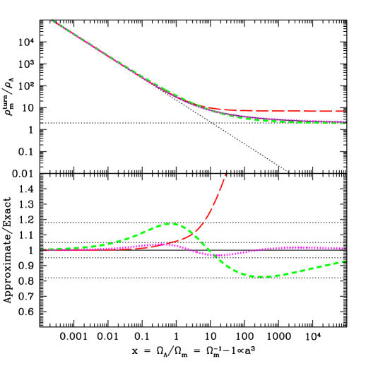
Figure 13: The top panel shows the turnaround (minimum) matter density $\rho_{\rm turn}$ of a top hat halo as a function of the time $x$ when its collapses. The virial density of the resulting dark matter halo is $\rho_{\rm vir}\sim 8\rho_{\rm turn}$. The solid curve is the exact result, with the asymptotic behavior $\rho_{\rm turn}\to 9\pi^{2}\rho_{\rm m}/4x$ as $x\to 0$ and $\rho_{\rm turn}\to 2\rho_{\Lambda}$ as $x\to\infty$ (dotted lines). The three analytic fits correspond to equation (74) (short-dashed), equation (75) (dotted) and that of BryanNorman98 ; Bullock99 , which in our notation is $(18\pi^{2}/x+18\pi^{2}-82-39x/(1+x))/8$. The first two are seen to be accurate to better than 18% and 4% respectively (bottom panel).

We will now derive the virial density of a halo formed at time $x$ in a $\Lambda$CDM universe, generalizing the standard result $\rho_{\rm vir}\sim 18\pi^{2}\rho_{m}(x)$. Whereas past work on this subject BryanNorman98 ; Bullock99 has focused on accurate numerical fits to the observationally relevant present epoch and recent past ($x\mathrel{\hbox to0.0pt{\lower 3.0pt\hbox{$\mathchar 536\relax$}\hss}\raise 2.0pt\hbox{$\mathchar 316\relax$}}1$), we need a formula accurate for all times $x$.

Consider first the evolution of a top hat overdensity in a $\Lambda$CDM universe. By Birkhoff’s theorem, it is given by the Friedman equation corresponding to a closed universe:

$${3H^{2}\over 8\pi G}=\rho_{\Lambda}+\rho_{\rm m}-{k\over a^{2}}=(1-{\kappa\over A^{2}}+{1\over A^{3}})\rho_{\Lambda},$$ (70)

where we have defined a dimensionless scale factor $A\equiv(\rho_{\Lambda}/\rho_{\rm m})^{1/3}$ and a dimensionless curvature parameter $\kappa\equiv(A/a)^{2}k$. One readily finds that this will give $H=0$ and recollapse for any curvature $\kappa>\kappa_{\rm min}\equiv{3/2^{2/3}}\sim 1.8899$, so the scale factor $A_{\rm max}(\kappa)$ at turnaround is given by solving equation (70) for $H=0$, i.e., by numerically finding the smallest positive root $A$ of the cubic polynomial $A^{3}-\kappa A+1=0$. $A_{\rm max}(\kappa_{\rm min})=2^{-1/3}\approx 0.79$, falling off as $A_{\rm max}(\kappa)\approx 1/\kappa$ for $\kappa\gg 1$.

The age of the universe $t_{\rm turn}$ when the top hat turns around is given by integrating $dt=d\ln A/(d\ln A/dt)=dA/(AH)$ using equation (70), i.e.,

$$H_{\Lambda}t_{\rm turn}(\kappa)=\int_{0}^{A_{\rm max}(\kappa)}{dA\over\sqrt{A^{2}-\kappa+{1\over A}}},$$ (71)

where $H_{\Lambda}\equiv(8\pi G\rho_{\Lambda}/3)^{1/2}$. For the unperturbed background $\Lambda$CDM universe where we used $x$ as a more convenient time variable, we have $\kappa=0$ and $A=x_{\rm turn}^{1/3}$ when the overtensity turns around, giving $t_{\rm turn}$ in terms of $x_{\rm turn}$:

$$H_{\Lambda}t_{\rm turn}(x_{\rm turn})=\int_{0}^{x_{\rm turn}^{1/3}}{dA\over\sqrt{A^{2}+{1\over A}}}.$$ (72)

Eliminating $t_{\rm turn}$ between equations (71) and (72) allows us to numerically compute the function $\kappa(x_{\rm turn})$.

Putting everything together now allows us to numerically compute the density of our top hat overdensity at turnaround: Since $\rho_{\rm m}=\rho_{\Lambda}/A^{3}$, we have

$$\rho_{\rm turn}(x_{\rm turn})={\rho_{\Lambda}\over A_{\rm max}(\kappa(x_{\rm turn}))^{3}}.$$ (73)

The result is shown in Figure 13 together with three analytic fitting functions. The simple fit

$$\rho_{\rm turn}(x)\approx 2\left[\left({9\pi^{2}\over 8x}\right)^{107\over 200}+1\right]^{200\over 107}\rho_{\Lambda}$$ (74)

is accurate to better than 18% for all $x$ and becomes exact in the two limits $x\to 0$ and $x\to\infty$. The fit

$$\rho_{\rm turn}(x)\approx\left({9\pi^{2}\over 4x}+{6.6\over x^{0.3}}+2\right)\rho_{\Lambda}$$ (75)

is accurate to better than 4% for all $x$ and also becomes exact in both limits, but we will nontheless use the less accurate equation (74) because it is analytically invertible and still accurate enough for our purposes. Applying the virial theorem gives a characteristic virial density $\rho_{\rm vir}\sim 8\rho_{\rm turn}$, with a weak additional dependence on $\rho_{\Lambda}$ Lahav91 . This means that a halo that virialized at time $x$ has

$$\rho_{\rm vir}\sim\left[(18\pi^{2}\rho_{\rm m}(x))^{107\over 200}+(16\rho_{\Lambda})^{107\over 200}\right]^{200\over 107},$$ (76)

i.e., essentially the larger of the two terms $18\pi^{2}\rho_{\rm m}(x)$ and $16\rho_{\Lambda}$. Inverting this, we obtain

$$x\sim{9\pi^{2}\over 8}\left[\left({\rho_{\rm vir}\over 16\rho_{\Lambda}}\right)^{107\over 200}-1\right]^{-{200\over 107}}.$$ (77)

A familiar quantity in the literature is the collapse overdensity $\Delta_{c}\equiv\rho_{\rm vir}/\rho_{m}=\rho_{\rm vir}x/\rho_{\Lambda}$, equaling $18\pi^{2}\approx 178$ for a flat $\rho_{\Lambda}=0$ universe. Using equation (74), equation (75) and the fit in Bullock99 to the calculations of BryanNorman98 gives

$$\Delta_{c}(x) \approx 18\pi^{2}\left[1+\left({8x\over 9\pi^{2}}\right)^{107\over 200}\right]^{200\over 107},$$ (78)

$$\Delta_{c}(x) \approx 18\pi^{2}+{52.8x^{0.7}}+16x,$$ (79)

$$\Delta_{c}(x) \approx 18\pi^{2}+(18\pi^{2}-82)x-39{x^{2}\over 1+x},$$ (80)

respectively. Figure 13 shows that our approximations substantially improve the accuracy, equation (79) being good to 4%. This improvement not surprising, since the approximation (80) was not designed to work well for $x\gg 1$.

References

- (1) V. F. Weisskopf, Science, 187, 605 (1975)
- (2) B. Carr and M. J. Rees, Nature, 278, 605 (1979)
- (3) D. Scott, astro-ph/0510731, 2005
- (4) S. Eidelman et al., Phys. Lett. B, 592, 1 (2004)
- (5) R. N. Mohapatra, hep-ph/0411131, 2004
- (6) M. Tegmark, JCAP, 2005-4, 1 (2005)
- (7) F. Wilczek, Phys. Today, 58/10, 12 (2005)
- (8) F. Wilczek, Phys. Today, 59/1, 10 (2006)
- (9) B. Carter 1974, in IAU Symposium 63, ed. S. Longair (Reidel: Dordrecht)
- (10) J. D. Barrow and F. J. Tipler, The Anthropic Cosmological Principle (Clarendon Press: Oxford, 1986)
- (11) M. J. Rees, Our Cosmic Habitat (Princeton Univ. Press: Princeton, 2002)
- (12) N. Bostrom, Anthropic Bias: Observation Selection Effects in Science and Philosophy (Routledge: New York, 2002)
- (13) M. Tegmark, astro-ph/0302131, 2003
- (14) A. Aguirre and M. Tegmark, hep-th/0409072, 2004
- (15) G. L. Kane, M. J. Perry, and A. N. Zytkow, New Astron., 7, 45 (2002)
- (16) P. Danies, Mod.Phys.Lett. A, 19, 727 (2004)
- (17) C. J. Hogan, astro-ph/0407086, 2004
- (18) W. R. Stoeger, G. F. R Ellis, and U. Kirchner, astro-ph/0407329, 2004
- (19) A. Aguirre, astro-ph/0506519, 2005
- (20) M. Livio and M. J. Rees, Science, 309, 1022 (2005)
- (21) S. Weinstein, hep-th/0508006, 2005
- (22) S. Weinberg, hep-th/0511037, 2005
- (23) M. Tegmark, Ann. Phys., 270, 1 (1998)
- (24) F. Wilczek, Phys. Today, 57/1, 10 (2005)
- (25) A. D. Linde, Particle Physics and Inflationary Cosmology (Harwood: Switzerland, 1990)
- (26) A. Vilenkin, PRD, 27, 2848 (1983)
- (27) A. A. Starobinsky, Fundamental Interactions (MGPI Press, Moscow: p.55, 1984)
- (28) A. A. Starobinsky 1986, in Current Topics in Field Theory, Quantum Gravity and Strings, Lecture Notes in Physics, vol. 246, ed. H. J. de Vega H J and N. Sanchez (Springer: Heidelberg.)
- (29) A. S. Goncharov, A. D. Linde, and V. F. Mukhanov, Int. J. Mod. Phys. A, 2, 561 (1987)
- (30) D. S. Salopek and J. R. Bond, PRD, 43, 1005 (1991)
- (31) A. D. Linde, D. A. Linde, and A. Mezhlumian, Phys. Rev. D, 49, 1783 (1994)
- (32) A. D. Linde, PLB, 201, 437 (1988)
- (33) F. Wilczek, hep-ph/0408167, 2004
- (34) A. D. Linde 2004, to appear in “Parallel Universes”, B. Carr, ed., Cambridge Univ. Press
- (35) R. Bousso and J. Polchinski, JHEP, 6, 6 (2000)
- (36) J. L. Feng, J. March-Russell, S. Sethi, and Wilczek F, Nucl. Phys. B, 602, 307 (2001)
- (37) S. Kachru, R. Kallosh, A. Linde, and S. P. Trivedi, PRD, 68, 046005 (2003)
- (38) L. Susskind, hep-th/0302219, 2003
- (39) S. Ashok and M. R. Douglas, JHEP, 401, 60 (2004)
- (40) A. D. Linde and A. Mezhlumian, Phys. Lett. B, 307, 25 (1993)
- (41) J. Garcia-Bellido, A. D. Linde, and D. A. Linde, PRD, 50, 730 (1994)
- (42) J. Garcia-Bellido and A. D. Linde, PRD, 51, 429 (1995)
- (43) A. Linde, D. Linde, and A. Mezhlumian, Phys. Lett. B, 345, 203 (1995)
- (44) A. Vilenkin, PRL, 74, 846 (1995)
- (45) S. Winitzki and A. Vilenkin, PRD, 53, 4298 (1996)
- (46) A. D. Linde and A. Mezhlumian, PRD, 53, 4267 (1996)
- (47) A. D. Linde, D. A. Linde, and A. Mezhlumian, Phys. Rev. D, 54, 2504 (1996)
- (48) A. Vilenkin and S. Winitzki, PRD, 55, 548 (1997)
- (49) A. Vilenkin, PRL, 81, 5501 (1998)
- (50) A. Vanchurin, A. Vilenkin, and S. Winitzki, PRD, 61, 083507 (2000)
- (51) J. Garriga and A. A. Vilenkin, PRD, 64, 023507 (2001)
- (52) J. Garriga, D. Perlov-Schwartz, A. Vilenkin, and S. Winitzki, hep-th/0509184, 2005
- (53) I. G. Irastorza, hep-ex/0509004, 2005
- (54) J. A. De Freitas Pacheco and S. Peirani, astro-ph/0503380, 2005
- (55) R. D. Peccei and H. R. Quinn, PRL, 38, 1440 (1977)
- (56) S. Weinberg, PRL, 40, 223 (1978)
- (57) F. Wilczek, PRL, 40, 279 (1978)
- (58) J. Preskill, M. Wise, and F. Wilczek, Phys. Lett. B, 120, 127 (1983)
- (59) L. Abbott and P. Sikivie, Phys. Lett. B, 120, 133 (1983)
- (60) M. Dine and W. Fischler, Phys. Lett. B, 120, 137 (1983)
- (61) M. Pospelov and A. Ritz, Annals of Physics, 318, 119 (2005)
- (62) M. S. Turner and F. Wilczek, PRL, 66, 5 (1991)
- (63) A. D. Linde, PLB, 259, 38 (1991)
- (64) T. Banks and M. Dine, Nucl. Phys. B, 505, 445 (1997)
- (65) T. Banks, M. Dine, and M. Graesser, PRD, 68, 075011 (2003)
- (66) S. D. Burns, astro-ph/9711303, 1997
- (67) P. fox, A. Pierce, and S. Thomas, hep-th/0409059, 2004
- (68) H. V. Peiris et al., ApJS, 148, 213 (2003)
- (69) K. Moodley, M. Bucher, J. Dunkley, P. G. Ferreira, and C. Skordis, PRD, 70, 103520 (2004)
- (70) M. Kawasaki and T. Yanagida, Prog.Theor.Phys., 97, 809 (1997)
- (71) M. Y. Khlopov and S. G. Rubin, Cosmological Pattern of Microphysics in the Inflationary Universe (Kluwer: Dordrecht, 2005)
- (72) G. Jungman, M. Kamionkowski, and K. Griest, Phys.Rep., 267, 195 (1996)
- (73) J. L. Feng, astro-ph/0511043, 2005
- (74) N. Arkani-Hamed and Dimopoulos S, JHEP, 506, 073 (2005)
- (75) C. J. Hogan, Rev.Mod.Phys., 72, 1149 (2000)
- (76) V. Agrawal, S. M. Barr, J. F. Donoghue, and D. Seckel, PRD, 57, 5480 (1998)
- (77) V. Agrawal, S. M. Barr, J. F. Donoghue, and D. Seckel, PRL, 80, 1822 (1998)
- (78) F. Hoyle, ApJS, 1, 121 (1954)
- (79) H. Oberhummer, A. Csoto, and H. Schlattl, Science, 289, 88 (2000)
- (80) T. E. Jeltema and M. Sher, PRD, 61, 017301 (2000)
- (81) J. Garriga and A. Vilenkin, astro-ph/0508005, 2005
- (82) A. Linde and V. Mukhanov, astro-ph/0511736, 2005
- (83) M. Tegmark, A. Vilenkin, and L. Pogosian, astro-ph/0304536, 2003
- (84) L. Pogosian, A. Vilenkin, and M. Tegmark, JCAP, 407, 5 (2004)
- (85) M. Tegmark and M. J. Rees, ApJ, 499, 526 (1998)
- (86) W. H. Press and P. Schechter, ApJ, 187, 425 (1974)
- (87) D. J. Eisenstein and W. Hu, ApJ, 511, 5 (1999)
- (88) S. Weinberg, PRL, 59, 2607 (1987)
- (89) U. Seljak et al., astro-ph/0407372, 2004
- (90) U. Seljak, and M. Zaldarriaga, ApJ, 469, 437 (1996)
- (91) D. N. Spergel et al., ApJS, 148, 175 (2003)
- (92) M. Tegmark et al., PRD, 69, 103501 (2004)
- (93) O. Lahav, P. B. Lilje, J. R. Primack, and M. J. Rees, MNRAS, 251, 128 (1991)
- (94) G. Bryan and M. Norman, ApJ, 495, 80 (1998)
- (95) J. Bullock et al., MNRAS, 321, 559 (2001)
- (96) J. Binney, ApJ, 215, 483 (1977)
- (97) M. J. Rees and J. P. Ostriker, MNRAS, 179, 541 (1977)
- (98) S. D. M White and M. J. Rees, MNRAS, 183, 341 (1978)
- (99) A. Blanchard, D. Valls-Gabaud, and G. Mamon A, A&A, 264, 365 (1992)
- (100) E. Ripamonti and T. Abel, astro-ph/0507130, 2005
- (101) D. Galli and F. Palla, A& A, 335, 403 (1998)
- (102) A. Toomre, ApJ, 139, 1217 (1964)
- (103) S. M. Fall and G. Efstathiou, MNRAS, 193, 189 (1980)
- (104) J. F. Navarro, C. S. Frenk, and S. D. M White, ApJ, 490, 493 (1997)
- (105) A. Aguirre, ApJ, 521, 17 (1999)
- (106) P. J. E Peebles, The Large-Scale Structure of the Universe (Princeton Univ. Press: Princeton, 1980)
- (107) A. D. Linde 1987, in 300 Years of Gravitation, ed. S. Hawking and W. Israel (Cambridge University Press: Cambridge)
- (108) G. Efstathiou, MNRAS, 274, L73 (1995)
- (109) H. Martel, P. R. Shapiro, and S. Weinberg, ApJ, 492, 29 (1998)
- (110) J. Garriga and A. Vilenkin, PRD, 67, 043503 (2003)
- (111) S. Hellerman and S. Walcher, hep-th/0508161, 2005
- (112) A. P. Lightman, Am. J. Phys., 52, 211 (1984)
- (113) P. Nurmi, M. J. Valtonen, and J. Q. Zheng, MNRAS, 327, 1367 (2001)
- (114) J. Byl, Moon & Planets, 29, 121 (1983)
- (115) P. Hut, W. Alvarez, W. P. Elder, E. G. Kauffman, T. Hansen, G. Keller, E. M. Shoemaker, and P. R. Weissman, Nature, 329, 118 (1987e)
- (116) L. W. Alvarez, W. Alvarez, F. Asaro, and H. V. Michel, Science, 208, 1095 (1980)
- (117) G. R. Byerly, D. R. Lowe, J. L. Wooden, and X. Xie, Science, 297, 1325 (2002)
- (118) K. J. Meech, O. R. Hainaut, and B. G. Marsden, Icarus, 170, 463 (2004)
- (119) G. Gonzalez, MNRAS, 308, 447 (1999)
- (120) A. Melott, B. C. Thomas, D. P. Hogan, L. M. Ejzak, and C. H. Jackman, Geophys. Res. Lett., 32, L14808 (2005)
- (121) J. Garriga, M. Livio, and A. Vilenkin, PRD, 61, 23503 (2000)
- (122) M. L. Graesser, S. D. H Hsu, A. Jenkins, and M. B. Wise, PLB, 600, 15 (2004)
- (123) M. Douglas 2005, private communication.