Marked correlations in galaxy formation models

Abstract

The two-point correlation function has been the standard statistic for quantifying how galaxies are clustered. The statistic uses the positions of galaxies, but not their properties. Clustering as a function of galaxy property, be it type, luminosity, color, etc., is usually studied by analysing a subset of the full population, the galaxies in the subset chosen because they have a similar range of properties. We explore an alternative technique—marked correlations—in which one weights galaxies by some property or ‘mark’ when measuring clustering statistics. Marked correlations are particularly well-suited to quantifying how the properties of galaxies correlate with their environment. Therefore, measurements of marked statistics, with luminosity, stellar mass, color, star-formation rate, etc. as the mark, permit sensitive tests of galaxy formation models. We make measurements of such marked statistics in semi-analytic galaxy formation models to illustrate their utility. These measurements show that close pairs of galaxies are expected to be red, to have larger stellar masses, and to have smaller star formation rates. We also show that the simplest unbiased estimator of the particular marked statistic we use extensively is very simple to measure—it does not require construction of a random catalog—and provide an estimate of its variance. Large wide-field surveys of the sky are revolutionizing our view of galaxies and how they evolve. Our results indicate that application of marked statistics to this high quantity of high-quality data will provide a wealth of information about galaxy formation.

1 Introduction

It has been thirty five years since Totsuji & Kihara (1969) published their measurement of the galaxy correlation function. Since then, measurements in ever larger catalogs have shown their initial estimate of $\xi(r)\propto r^{-1.8}$ on scales smaller than about ten Megaparsecs was accurate (e.g., Maddox et al. 1990; Percival et al. 2001; Hamilton & Tegmark 2002; Connolly et al. 2002). Recent work in the 2dFGRS (Colless et al. 2001) and SDSS (Abazajian et al. 2005) surveys has shown definitively that clustering depends on galaxy type, color and luminosity (Norberg et al. 2002; Zehavi et al. 2002, 2005). In what follows, we will speak of any combination of properties which distinguish galaxies from one another as marks.

Marks can take discrete or continuous values, and they may be scalars or vectors. The traditional morphological type of a galaxy is a discrete scalar mark. Luminosity, color, X-ray hardness, AGN activity and star formation rate are all examples of continuous scalar marks. A typical neural network classifies morphological types as a list of probabilities ${{\mbox{\boldmath$p$}}}=(p_{1},\cdots,p_{n})$, where $p_{i}$ is the probability a galaxy is of type $T_{i}$ (e.g., Storrie-Lombardi et al. 1992; Lahav et al. 1996). If one classified galaxies using this probability vector (rather than simply using the type $T_{i}$ which had the largest $p_{i}$), then morphological type is a vector mark. Principal component analyses of galaxy spectra output a vector ${{\mbox{\boldmath$c$}}}=(c_{1},\cdots,c_{n})$, where $c_{i}$ denotes the contribution of eigenspectrum $i$ to the object’s spectrum (e.g. Connolly et al. 1995). The spectral classification $c$ can, therefore, be used as a vector mark.

In most analyses to date (e.g., Hamilton 1988; Mo, Börner & Zhou 1989; Willmer, da Costa & Pellegrini 1998; Benoist et al. 1999; Norberg et al. 2002; Zehavi et al. 2005), the parent galaxy catalog is cut into subsamples based on the mark (most often morphological type or luminosity), and the clustering in the subsample is studied by treating each galaxy in it equally. That is to say, the mark is used to define the subsample, but is not considered further. This is equivalent to relabeling all marks to be ‘zeros’ or ‘ones’, depending on whether or not the value of the mark crossed a threshold value, and then computing the correlation function of the galaxies marked as ‘ones’. There are two reasons why this procedure is not ideal. First, the choice of critical threshold is somewhat arbitrary, particularly in the case of marks like luminosity and color which take a continuous range of values. Second, throwing away the actual value of the mark represents a loss of information. Therefore, one might well ask: Why not weight each galaxy by its actual mark, rather than relabelling to ones and zeros?

With the advent of large wide-field space– and ground–based surveys of the sky, many of the marks mentioned above can now be measured with sufficient precision that contamination by measurement error is not a serious concern. Indeed, many of these marks have been, or can be, reliably measured in a number of datasets now available. For example, the luminosities in the 2MASS survey are expected to be indicators of total stellar mass; the ROSAT all sky survey can be used to estimate the hardness of the spectra of X-ray sources; the GALEX mission will provide estimates of star formation rates out to redshifts of order unity. The time is ripe to take advantage of the additional information provided by weighting each galaxy by its mark.

Marked correlations in the SSRS2, IRAS 1.2 Jy and PSCz surveys, using luminosity and/or type as mark were measured by Beisbart & Kerscher (2000). The marked correlations showed evidence that the luminosities of close pairs of galaxies were larger than the mean on separations larger than about $10h^{-1}$Mpc. Beisbart & Kerscher did not compare their measurements with specific model predictions, so their results have had less impact on galaxy formation models than they might otherwise have had.

Semi-analytic galaxy formation models (White & Rees 1979; White & Frenk 1991; Kauffmann et al. 1999; Somerville & Primack 1999; Cole et al. 2000; Springel et al. 2005) provide the basis for our current understanding of how and why different galaxy types are differently biased tracers of the dark matter field. They also provide a useful framework for seeing if simple models are consistent with the observed correlations between luminosity and velocity dispersion or circular velocity (Faber & Jackson 1976; Tully & Fisher 1977), morphology and density (Dressler 1980), morphology or density and star formation rate (Lewis et al. 2002; Gomez et al. 2003; Kauffmann et al. 2004), etc.

Although the predictions of these models depend on a number of free parameters, and they do not always provide perfect descriptions of the data, they have proven to be useful for gaining insight into how changes in the physics of galaxy formation affect the properties of the galaxy population. These models output a number of marks which are potentially observable. These include luminosity, size, velocity dispersion, morphology, star-formation rate, local density, and so on, and how these marks evolve. The main goal of the present paper is to measure various marked correlation functions in these models, so as to illustrate how marked statistics can provide direct physical insight into the processes of galaxy formation.

Section 2 introduces the family of pairwise marked correlation functions, and defines the particular generalization of the usual correlation function we will use. Section 3 shows measurements of various marked correlation functions made in semi-analytic models of galaxy formation. Section 4 discusses the effects of rescaling marks prior to measuring marked statistics. Such rescaling is necessary if one wishes to compare galaxy formation models with observations, if, as is often the case, the distribution of marks in the models is not the same as in the data. A final section summarizes our findings, and discusses some extensions. An Appendix provides a brief discussion of the bias and variance of our estimators of marked statistics (our estimators are unbiased, but they are not minimum variance). In essence, the estimator we use throughout this paper is particularly straightforward to implement because it does not require construction of a random catalog; in this respect, marked statistics are substantially easier to estimate than the usual unweighted correlation functions.

2 Marked statistics

Marked correlations measure the clustering of marks. Since the positions at which the marks are measured may themselves be clustered, marked statistics are defined in a way which accounts for this. This is the subject of Sections 2.1 and 2.4. Marked statistics are usually studied to see if marks depend on environment. Section 2.6 shows that marked statistics have another very useful application which has not been emphasized previously. Namely, different marks frequently correlate with each other: marked statistics can be used to quantify if the correlations between marks depend on environment.

2.1 Definitions

For example, let $\bar{\rho}$ denote the mean density of particles, and let $\bar{m}$ denote the mean mark, averaged over all particles. Now consider a particle with mark larger than this mean value. Are the particles neighbouring it also likely to have larger marks? One way to quantify how likely this is is to compute the ratio of the mean mark to $\bar{m}$ of pairs of particles as a function of pair separation. The typical number of pairs at separation $r$ is $\bar{\rho}^{2}[1+\xi(r)]$, where $\xi$ is the two point correlation function. Therefore, the mean mark is

$${\cal M}_{1}(r) = {\sum[m({{\mbox{\boldmath$x$}}})+m({{\mbox{\boldmath$y$}}})]\,{\cal I}(|{{\mbox{\boldmath$x$}}}-{{\mbox{\boldmath$y$}}}|-r)\over 2\bar{m}\ \sum{\cal I}(|{{\mbox{\boldmath$x$}}}-{{\mbox{\boldmath$y$}}}|-r)}$$ (1)

$$= {\sum[m({{\mbox{\boldmath$x$}}})+m({{\mbox{\boldmath$y$}}})]\,{\cal I}(|{{\mbox{\boldmath$x$}}}-{{\mbox{\boldmath$y$}}}|-r)\over 2\bar{m}\ \bar{\rho}^{2}[1+\xi(r)]},$$

where ${\cal I}(x)=0$ unless $x=0$, and the sum is over all galaxy pairs. We have divided by $\bar{m}$, so ${\cal M}_{1}(r)=1$ for all $r$ if there are no correlations between marks. Analogously, the $n$th-order mark is defined by

$${\cal M}_{n}(r)={\sum[m({{\mbox{\boldmath$x$}}})+m({{\mbox{\boldmath$y$}}})]^{n}\,{\cal I}(|{{\mbox{\boldmath$x$}}}-{{\mbox{\boldmath$y$}}}|-r)\over(2\bar{m})^{n}\ \bar{\rho}^{2}[1+\xi(r)]}.$$ (2)

In what follows, we will concentrate on the mean square mark

$${\cal M}_{2}(r)={\sum[m^{2}({{\mbox{\boldmath$x$}}})+m^{2}({{\mbox{\boldmath$y$}}})+2m({{\mbox{\boldmath$x$}}})m({{\mbox{\boldmath$y$}}})]\,{\cal I}(|{{\mbox{\boldmath$x$}}}-{{\mbox{\boldmath$y$}}}|-r)\over 4\bar{m}^{2}\ \bar{\rho}^{2}[1+\xi(r)]}.$$

If all the marks are the same, then ${\cal M}_{2}=1$. If the marks are independent, with mean $m_{1}=\bar{m}$ and mean square $m_{2}$, then ${\cal M}_{2}=(m_{2}+m_{1}^{2})/2\bar{m}^{2}=(m_{2}/\bar{m}^{2}+1)/2$. To see why this is sensible, compute the variance: ${\cal V}ar(r)={\cal M}_{2}(r)-{\cal M}_{1}(r)^{2}=(m_{2}/\bar{m}^{2}-1)/2$. This shows that ${\cal V}ar$ equals half the variance of the individual marks, as it should (recall it is the variance of one half times the sum of two independent marks).

Two types of terms contribute to ${\cal M}_{2}$. The term which involves a product of two marks is proportional to

$$M(r)\equiv{\sum m({{\mbox{\boldmath$x$}}})m({{\mbox{\boldmath$y$}}})\,{\cal I}(|{{\mbox{\boldmath$x$}}}-{{\mbox{\boldmath$y$}}}|-r)\over\bar{m}^{2}\,\sum{\cal I}(|{{\mbox{\boldmath$x$}}}-{{\mbox{\boldmath$y$}}}|-r)}\equiv{1+W(r)\over 1+\xi(r)},$$ (3)

where we have defined $W(r)$ for the following reason. The only difference between the sums in the numerator and denominator is that, in the numerator, the $i$th particle contributes a weight $m_{i}/\bar{m}$, whereas in the denominator, the weight is unity for all particles. Since the denominator is one plus the usual unweighted correlation function, the numerator can be thought of as being one plus a weighted correlation function. In effect, the denominator divides-out the contribution to the weighted correlation function which comes from the spatial distribution of the points, leaving only the contribution from the fluctuations of the marks.

2.2 Estimators and the weighted correlation function

There are a number of reasons why this ratio, $M(r)$, is the measure of marked correlations on which we will concentrate. First, fast estimators of unweighted correlations (which account for edge effecs, etc.) have been available for some time (e.g., Peebles 1980). If we write the usual estimator for the unweighted correlation function as $DD/RR$, then the weighted correlation function is $WW/RR$, and the marked statistic above is simply $WW/DD$. This has two important implications. First, allowing for weights requires only a simple modification of algorithms which estimate unweighted correlations (e.g. Moore et al. 2000). Second, because edge effects appear in both the numerator and denominator, this marked correlation ratio is less sensitive to edge effects than is, e.g., the $DD/RR$ estimator of the unweighted correlation function (e.g. Beisbart & Kerscher 2000). Perhaps more importantly, note that the $RR$ factor cancels out, so that the marked statistic can be estimated without constructing a random catalog; this significantly reduces the computational burden for estimating the statistic. Third, errors on the measurement are readily estimated, as described in Appendix A. (It is relatively common to approximate the errors by remaking the measurement after randomizing the marks, and repeating a large number of times. We show that this is a reasonable approximation on the small scales where we find the most interesting results, but leads to an underestimate of the true errors on larger scales.) And finally, it is by thinking of marked correlations as this ratio of weighted to unweighted correlations that one is able to construct theoretical models of marked correlations (Sheth, Abbas & Skibba 2004; Sheth 2005).

2.3 Measurement errors

If the mark is not perfectly measured, so the observed mark $o_{i}$ of object $i$ is $o_{i}=m_{i}+e_{i}$, where $e_{i}$ is the error in the measurement, then the measured marked correlation function will be $M_{o}(r)=\langle(m_{i}+e_{i})(m_{j}+e_{j})|r\rangle$ , where the notation denotes the average over all pairs $i$ and $j$ separated by $r$. Thus, $M_{o}(r)=M_{m}(r)+M_{e}(r)$ plus a term which allows for the fact that the mark of one object is correlated with the error made in measuring the marks of the other objects. If there is no such correlation, and if the mean measurement error for objects does not depend on position, and if the errors themselves are uncorrelated, then $M_{o}(r)=M_{m}(r)$: in this case, the measured marked correlation will be an unbiased representation of the true correlation. Of course, the precision with which this marked correlation function can be determined will depend on the amplitudes of the $e_{i}$s. Appendix A provides a more detailed discussion.

2.4 Normalization

The expressions above follow the conventions in the statistical literature (e.g. Stoyan 1984; Stoyan & Stoyan 1994), and so normalize the marks by the mean mark. There is no apriori reason for this choice. For instance, we could have chosen to normalize by the rms value instead. In models where large scale correlations are expected to be small, our convention makes the large scale limit $M(r)\to 1$, which is intuitively easy to understand. Normalizing by the square root of the mean squared mark instead makes the amplitude of the small-scale signal easier to understand, since this convention would have $M(r\to 0)\to 1$, but then the large scale value would depend on the ratio of the mean and rms values of the marks. This convention might be useful if one is interested in studying marked statistics in a density field which was obtained by smoothing the mark-weighted point distribution.

Moreover, the expressions above implicitly assume that $\bar{m}$ is not zero. If marks are not positive definite, then $\bar{m}\neq 0$ is not guaranteed, and one may well have to normalize by the rms value. To avoid this complication, in what follows, we will only consider marks which are positive definite. Analysis in Section 4 suggests that monotonic rescalings of the marks will not seriously compromise their use. Thus, for instance, when we use galaxy colors (which are proportional to the log of the ratio of the luminosity in two different wavebands) as marks, we use the ratio of the luminosities, rather than the log of this ratio.

2.5 Cross-correlations

So far, we have implicitly assumed that the mark used for both particles was the same. There is no reason why we could not have used different marks for the two particles of each pair. For example, we could use effective radius and local density as two marks to study if galaxies in denser regions are smaller or larger than average. Marked cross-correlations could also be used to study if star formation rates in galaxies are affected by AGN activity in their neighbors. To estimate cross correlations of this type, the expressions given previously remain true, with the replacements $m({{\mbox{\boldmath$x$}}})m({{\mbox{\boldmath$y$}}})/\bar{m}^{2}\to m_{a}({{\mbox{\boldmath$x$}}})m_{b}({{\mbox{\boldmath$y$}}})/\bar{m}_{a}\bar{m}_{b}$, where the subscripts $a$ and $b$ denote the two different types of marks.

2.6 Correlations between marks

Many galaxy observables correlate with each other: e.g., the velocity dispersion of a galaxy correlates with its size, luminosity, and color. Marked statistics provide a simple way to see if such correlations depend on environment. Note that this differs from the previous subsection which described marked cross-correlations between a mark of one galaxy and another mark of its neighbour; here we are interested in quantifying how the correlation between two (or more) marks of the same galaxy depends on the surrounding environment.

Suppose each galaxy has two weights, $m$ and $w$, and that a plot of the two versus one another (each galaxy is a point in this two-dimensional plot) shows a correlation, but there is scatter around the mean correlation. Let $w=f(m)$ denote this mean correlation. A question which often arises is: Does the scatter correlate with environment? If we write $w_{i}=f_{i}+e_{i}$, where $f_{i}\equiv f(m_{i})$, then

$$M_{w}(r) = \left\langle{w_{i}\over\bar{w}}{w_{j}\over\bar{w}}\Big{|}r\right\rangle=\left\langle{[f_{i}+e_{i}]\over\bar{f}}{[f_{j}+e_{j}]\over\bar{f}}\Big{|}r\right\rangle$$

$$= \left\langle{f_{i}f_{j}+f_{i}e_{j}+f_{j}e_{i}+e_{i}e_{j}\over\bar{f}^{2}}\Big{|}r\right\rangle,$$

where the notation is intended to show that the averages are over all pairs with separation $r$. Evidently, $M_{w}$ is a (suitably weighted) combination of $M_{f}$, $M_{e}$, and the cross-correlation between $f$ and $e$. If the amount $e_{i}$ by which galaxy $i$ scatters from the mean $w-m$ relation is independent of the marks $m_{j}$ of the other galaxies, then $\langle e_{i}f_{j}|r\rangle=\langle e_{i}|r\rangle\langle f_{j}|r\rangle$ and $\langle e_{i}e_{j}|r\rangle=\langle e_{i}|r\rangle\langle e_{j}|r\rangle$. If the scatter is independent of environment, then $\langle e_{i}|r\rangle=0$ for all $r$. This shows that, if there is no correlation in the scatter, then $M_{w}(r)\to M_{f(m)}(r)$. Hence, one can determine if the correlation between marks depends on scale by comparing $M_{w}(r)$ with $M_{f(m)}(r)$. If $M_{m}(r)$ depends on scale, then $M_{w}=M_{m}$ only if $f(m)\propto m$. If $f(m)$ is a more complicated function of $m$, then $M_{w}$ differs from $M_{m}$ by a scale dependent factor even if $f(m)$ is independent of $r$.

2.7 An illustrative example

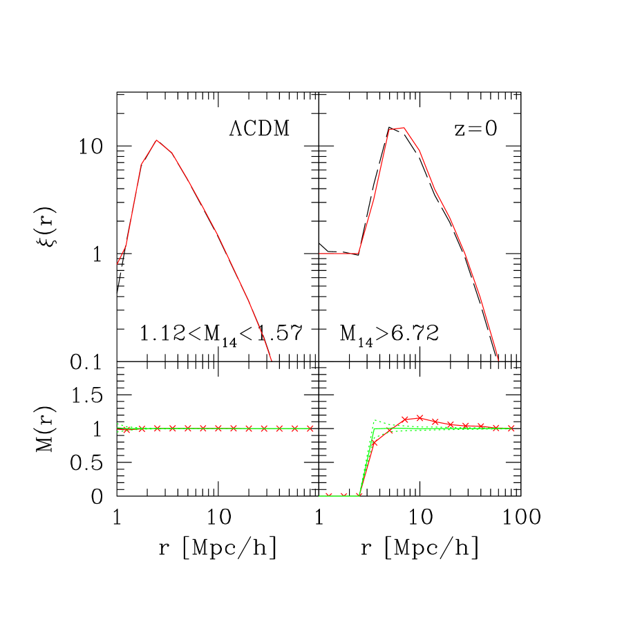
Figure 1: Correlation functions of massive halos in numerical simulations of a $\Lambda$CDM cosmology. Top panels show the number (dashed) and mass (solid) weighted correlation functions, and panels on the bottom show marked correlations (crosses). The dotted curves in the bottom panels show the mean plus and minus the standard deviation of measurements made after randomizing the marks.

Figure 1 shows an example of what marked correlation functions measure. The underlying point process was the halo distribution in the Hubble Volume simulation (Evrard et al. 2002) of a flat $\Lambda$CDM cosmology ($\Omega_{0}=0.3,h=0.7,\sigma_{8}=0.9$). The dashed lines in the top panels show the unweighted correlation function of halos with masses in the range $1.12\times 10^{14}M_{\odot}/h\leq M\leq 1.57\times 10^{14}M_{\odot}/h$ (left, about $2\times 10^{5}$ halos) and greater than $6.72\times 10^{14}M_{\odot}/h$ (right, $2.5\times 10^{4}$ halos). The solid lines in the top panels show the result of weighting each halo by the ratio of its mass to the mean halo mass in the subsample when computing the correlation function. Comparison of the two panels shows that on large scales, the more massive halos are more strongly clustered. The decrease at small $r$ is a consequence of volume exclusion: halos do not overlap. The more massive halos occupy larger volumes, so volume exclusion matters (i.e., the correlation functions turn over) at larger scales in the panel on the right (this effect was discussed by Mo & White 1996, and quantified by Sheth & Lemson 1999).

Let $C(r)$ and $W(r)$ denote the dashed and solid curves in the top panels. The symbols with solid lines drawn through them in the bottom panels show the marked correlations $M(r)=[1+W(r)]/[1+C(r)]$, where the mark is the halo mass. There is no trend in the panel on the left, because the range of halo masses in it is small. As a result, almost all halos have the same mass, and hence the same mark. In contrast, the symbols in the panel on the right show a hump at 10$h^{-1}$Mpc, indicating that the most massive halos tend to have separations of about that scale.

One of the virtues of marked correlations is that there is a simple way to assess the statistical significance of such a feature. The approximately horizontal curves bounded by dotted lines in the bottom panels show the mean and the standard deviation around the mean when the same measurement is made after randomizing the marks. (The curves show results averaged over one hundred random realizations.) Comparison of the symbols with these randomized curves shows that the hump at 10$h^{-1}$Mpc in the panel on the right is statistically significant. (Appendix A provides a more careful discussion of the uncertainty on the measured statistic, and shows that this randomization procedure slightly mis-estimates the true scatter, since it assumes there are no correlations between the marks. However, since the correlations between marks we find are not very different from unity, this estimate based on randomization is not far from the true answer.)

Although $M(r)\approx 1$ at large scales, it drops below unity on scales smaller than $5h^{-1}$Mpc. This indicates that the halos which contribute pairs at small separations are the least massive subset of the population, as one would expect from volume exclusion. Notice that the marked correlations illustrated this effect without having to separate the catalog up into small bins in mass. Therefore, they allow a measurement of what is in this case a ‘mass segregation’ effect which is of greater statistical significance than it would be in any one of the smaller catalogs.

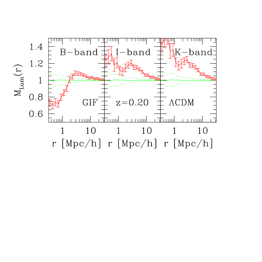
Figure 2: Marked correlations in the semi-analytic models with $B$, $I$ and $K$-band luminosity at $z=0.20$ as the mark. In each panel, jagged solid line shows the marked correlation, and error bars show the estimated uncertainty on the measurement derived in Appendix A. For comparison, horizontal line shows the mean obtained by averaging over one hundred realizations of the same measurement after randomizing the marks, and dotted lines show the standard deviation around this mean. When luminosity is the mark, the marked correlation is a strong function of wavelength.

3 Predictions of semi-analytic galaxy formation models

It is straightforward to make similar measurements, using various marks, in semi-analytic galaxy catalogs. In what follows, we will use the galaxy formation models of Kauffmann et al. (1999) to illustrate the sort of information that marked correlations provide. This is not because we feel other models are significantly worse, but because these model galaxy catalogs are available to the public (www.mpa-garching.mpg.de/Virgo). The models populate the dark matter distribution of the GIF simulation with galaxies: the background cosmology is a flat $\Lambda$CDM universe with $(\Omega,h,\sigma_{8})=(0.3,0.7,0.9)$, and the simulation box is a cubical comoving volume $141h^{-1}$Mpc on a side. All distances we show below are comoving.

We show measurements of marked statistics in these semi-analytic galaxy catalogs for subsamples of galaxies which contain more than $2\times 10^{10}h^{-1}M_{\odot}$ in stars. Such measurements are best thought of as being related to measurements in volume-limited, rather than magnitude-limited galaxy catalogs. At $z=0.2$ (this redshift was chosen to approximately match the median redshifts of the Two Degree Field Galaxy Redshift Survey and the Sloan Digital Sky Survey; c.f. Colless et al. 2001 and York et al. 2000) the semi-analytic galaxy catalog contains 14,665 objects. This number is about thirty percent smaller at $z=1.05$.

3.1 Luminosity

Figure 2 shows marked correlations in which luminosity was used as the mark. The various panels show measurements made in the semi-analytic models at $z=0.2$, at various wavelengths. In each panel, the jagged lines show the measurement, and error bars are estimated following the analysis in Appendix A. The figure shows clear evidence that the shape of the marked correlation function depends on wavelength. In all cases, $M_{\rm Lum}(r)$ falls gently at separations larger than about 3 Mpc, but the small scale behaviour is very different. It is interesting that this 3 Mpc scale is similar to that at which $\xi(r)$ shows a feature: this is the scale on which the statistic becomes dominated by pairs in separate halos.

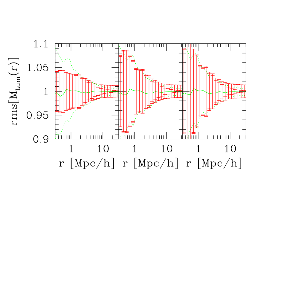
Figure 3: Comparison of various estimates of the uncertainty on the measurement; the three panels show the same set of marks as in Figure 2. Larger error bars show the full estimate from Appendix A; smaller error bars show the result of ignoring the contribution from equation (15). The standard deviation of the marked statistic measured in many (one hundred) realizations of the point distribution with randomized marks is shown by the dotted curves.

Comparison of the curves in the different panels shows that while all bands are reasonably similar on larger scales, the different bands are quite different from each other on smaller scales. In contrast to the redder band-passes, the marked correlation decreases with scale for the $B-$band. Evidently, the blue-band luminosities of galaxies with near neighbours (i.e., closer than a Mpc or so) are smaller than they are on average. Since the $B-$band luminosity is more sensitive to recent star formation than the $I-$ or $K-$bands, it is interesting to study what happens when star-formation rate is used as the mark.

We will make two additional points before we do so. First, although we have not shown this, we have found that if we restrict attention to any one band, then the amplitude of $M(r)$, especially on small scales, depends on the range of luminosities in the sample. In general, increasing the range of luminosities makes the small-scale dependence of $M(r)$ on $r$ more dramatic. The reason for this was hinted at in Section 2.4: if close pairs tend to have larger marks, then the amplitude of $M(r)$ depends on the range of luminosities in the sample.

Second, consider the horizontal solid line at $M\sim 1$ on all scales in each panel. This line shows the mean value of the statistic averaged over one hundred realizations of the catalog after randomizing the marks. The dotted lines show the standard deviation around this mean, and this standard deviation is sometimes used as an estimate of the error on the measurement of $M(r)$. Notice that the difference between the solid and dotted lines is similar to the size of the error bars on the measurement, indicating that this randomized-marks procedure of estimating errors does not grossly mis-estimate the true errors, at least on small scales.

Figure 3 provides a more direct comparison. Dotted curves show the error estimate from randomizing the marks. The two sets of error bars show the two contributions to the error estimate from Appendix A; the smaller estimate comes from ignoring the contribution from equation (15). On small scales, the dotted lines and full error bars are in good agreement, except in the $B$-band. In $B$-, $M(r)$ itself is smaller than unity, so the error estimate from Appendix A is also smaller than the one obtained from randomizing the marks. On larger scales, the estimate from Appendix A becomes significantly larger than the one from randomizing the marks. Since $M(r)$ itself is unity on these scales, this difference strongly suggests that our estimator, $WW/DD$, can be improved—while unbiased, is not minimum variance. This hypothesis is supported by the fact that, in this regime, the error estimate is dominated by the term in equation (15).

3.2 Colors and star-formation

Figure 4 shows the marked correlations of the same set of objects when color and star formation rate are used as marks (curves with error bars). As in the previous figure, the solid and dotted curves show the mean (averaged over one hundred realizations) and the standard deviation around the mean when the same measurement is made after randomizing the marks. The error estimates indicate that, at separations smaller than a Mpc or so, star formation rates are substantially lower than the mean, whereas the $V-I$ colors of close pairs are larger (i.e., redder) than the mean.

Comparison of the panels on the left with those on the right shows how the marked correlations evolve. Notice that the two marked correlations depend very differently on scale, suggesting that color and star-formation rate are biased very differently relative to the underlying dark matter distribution. On the other hand, the scale on which $M_{V-I}(r)$ suddenly increases is similar to the scale on which $M_{\rm SFR}(r)$ decreases, suggesting that similar physics gives rise to both effects.

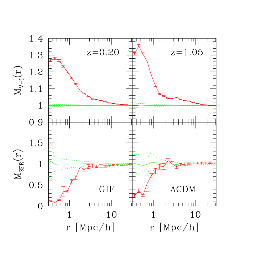
Figure 4: Marked correlations at $z=0.2$ and $z=1.05$ in the GIF semi-analytic galaxy formation models (Kauffmann et al. 1999). Top and bottom panels show results when the mark is restframe $V-I$ color and star formation rate, respectively. Curves with error bars show the marked correlations with associated uncertainties. Horizontal lines show the mean of one hundred realizations of the same measurement after randomizing the marks, and dotted lines show the standard deviation around this mean.

Why does this happen? Many close pairs come from galaxies in groups and clusters. In the models, such galaxies started forming their stars at higher redshifts than average. By the present time they are likely to have turned all the gas available to them into stars. Therefore, at low redshifts (e.g, $z<1$), the star formation rates in cluster galaxies are low, and their colors are red. Figure 4 shows that the marked correlation functions are sensitive to these effects. Since the top panel is weighted by $V-I$, and redder colors mean larger values of $V-I$, the marked correlations in the top panels show a dramatic increase on scales smaller than the typical virial radius of a large cluster. Since star formation within clusters has essentially switched off, the trend in the bottom is the opposite. Thus, in the models, it is no accident that the scale on which $M_{V-I}$ suddenly increases is similar to the scale on which $M_{\rm SFR}$ decreases.

Notice that the scale at which the two curves suddenly change is smaller at higher redshifts, and that the shift in scale is easily detected in both cases. This is not unexpected in models where star-formation is lowest in the most massive halos. Comparison with similar measurements in the data will show if these predictions of the models are correct. If not, the gastrophysics which has been used to model galaxy formation should be refined. For instance, GALEX observes galaxies out to redshifts of order unity, so it is well suited to performing this test.

3.3 Stellar mass and the mass-to-light ratio

We were prompted to study the star-formation rate because of the differences between the various panels of Figure 2. The discussion above suggests that the drop on scales smaller than an Mpc in the $B$-band is consistent with Figure 4 which showed a decrease in the star formation rate on small scales. Luminosities in the redder bands are less sensitive to recent star formation, so they are expected to be better tracers of the total stellar mass.

To illustrate, the curves with error bars in Figure 5 show marked correlations in the semi-analytic models at $z=0.2$ and $z=1.05$ when the stellar mass is used as mark. Comparison of the two panels shows that $M(r)$ evolves: at both redshifts, close pairs tend to more massive, but the scale on which this is a significant effect is smaller at high redshift. Moreover, the amplitude of $M(r)$ also evolves: stellar masses of close pairs at high redshift were not as different from the mean as they are today. The shift in amplitude and in scale means that similar measurements in data should provide sharp constraints on the models.

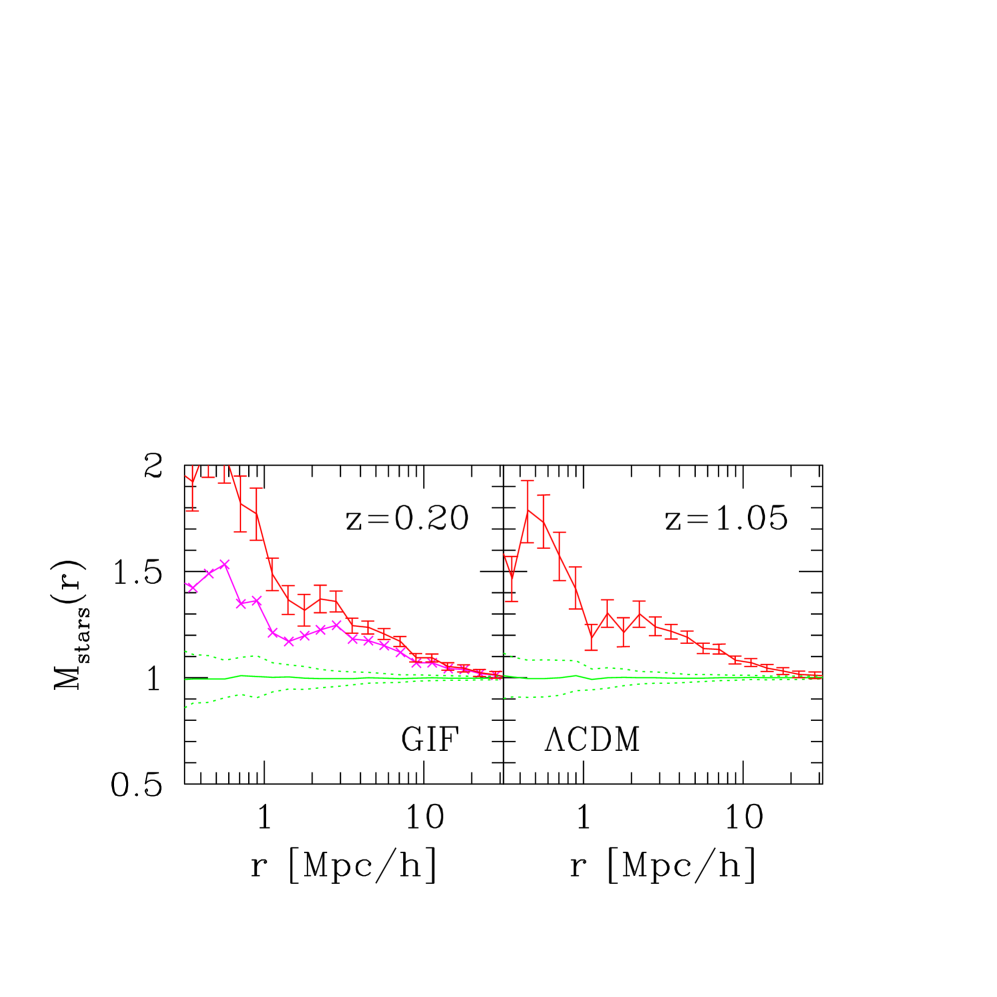
Figure 5: Marked correlations in which stellar mass is the mark (solid lines with error bars). For comparison, crosses in the panel on the left show what happens when $K-$band luminosity is the mark.

The crosses in the panel on the left show the result of using the $K-$band luminosity as the mark (for clarity, we have not shown the associated error estimates, since these are shown in Figure 2). Notice that the same bumps and wiggles are present for both $M_{K}$ and $M_{stars}$. This suggests that the two marks, $K$-band luminosity and stellar mass, do indeed reflect similar physics. The discussion in Section 2.6 indicates that comparison of these two marked correlations can be used to study if the correlation between stellar mass and $L_{K}$ is the same in all environments. In particular, if $L_{K}$ is linearly proportional to stellar mass, then the two marked correlations will be the same only if this correlation is independent of environment. (Specifically, if $L_{1}=aM_{1}+e_{1}$ with $\langle L\rangle=a\langle M\rangle$, then the marked statistic is $\langle L_{1}L_{2}|r\rangle/a^{2}\langle M\rangle^{2}=\langle M_{1}M_{2}|r\rangle/\langle M\rangle^{2}+2\langle M_{1}e_{2}|r\rangle/a\langle M\rangle^{2}+\langle e_{1}e_{2}|r\rangle/a^{2}\langle M\rangle^{2}$; the final two terms vanish only if the correlation is independent of environment.)

Figure 6 shows that $L_{K}\propto M_{\rm stars}$ (we have normalized each by their respective mean values across the population). Hence, the difference between the two curves in the left panel of Figure 5 suggests that the correlation between mass and light does depend on environment: close pairs tend to have larger mass-to-light ratios, suggesting that the mass-to-light ratio is larger in dense regions.

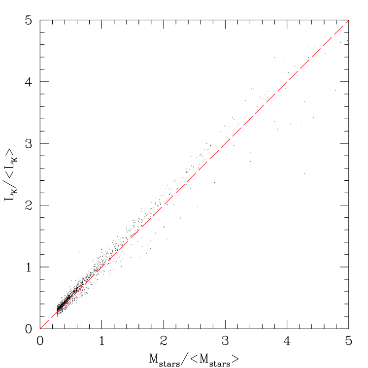
Figure 6: Correlation between $K$-band luminosity and stellar mass. Since this correlation is linear, the two marked correlations will be the same only if there are no environmental effects.

4 The effects of re-scaling

The semi-analytic models studied here do not match the observed distribution of galaxy properties precisely. For instance, these models do not match the SDSS luminosity function. On the other hand, they are reasonably successful at describing the luminosity dependence of clustering. For this reason, we envision that constraints on such models will take the following form. If the models successfully describe the luminosity dependence of clustering, then they have successfully identified the halos in which galaxies form. If marked correlations are not changed in any essential way if the absolute values of the weights are altered without changing the rank ordering, then marked statistics provide a way of determining if, in addition to correctly identifying the halos in which galaxies form, the models also determine the correct rank ordering of galaxy properties within halos.

For such a test to work, we must understand the effect that monotonic rescalings of the marks have on marked statistics. With this in mind, consider the following toy model. All galaxies come in either of two types of groups. Groups of one type contain $m_{1}$ galaxies, each having weight $W_{1}$, and the density run of galaxies around centres the group centers follows a Gaussian distribution with scale length $s_{1}\propto m_{1}^{1/3}$. Galaxies in groups of the second type follow a Gaussian distribution with scale length $s_{2}$, have weights $W_{2}$, and there are $m_{2}\propto s_{2}^{3}$ galaxies per group. Specifically, the density run around each type of group is $\rho(r)/\bar{\rho}=\Delta_{\rm nl}\,\exp(-r^{2}/2/s_{i}^{2})/\sqrt{2\pi}$, so $m_{i}=\Delta_{\rm nl}\bar{\rho}\,2\pi s_{i}^{3}$.

If $f$ denotes the fraction of groups of type 1, then the mean weight is $\bar{W}=[fm_{1}W_{1}+(1-f)m_{2}W_{2}]/[fm_{1}+(1-f)m_{2}]$. Hence, the normalized weights are $w_{1}=W_{1}/\bar{W}$ and $w_{2}=W_{2}/\bar{W}=1+(1-w_{1})(s_{1}/s_{2})^{3}\,f/(1-f)$. In this model,

$${1+W\over 1+\xi}={1+kfw_{1}^{2}\,{\rm e}^{-r^{2}/4s_{1}^{2}}+k(1-f)(s_{2}/s_{1})^{3}w_{2}^{2}\,{\rm e}^{-r^{2}/4s_{2}^{2}}\over 1+kf\,{\rm e}^{-r^{2}/4s_{1}^{2}}+k(1-f)(s_{2}/s_{1})^{3}\,{\rm e}^{-r^{2}/4s_{2}^{2}}}$$ (4)

where $k=[\Delta_{\rm nl}/4\sqrt{\pi}]/[f+(1-f)(s_{2}/s_{1})^{3}]$. Rescaling the marks corresponds to changing $W_{1}$; the fact that the marks are normalized then determines the rescaled value of $W_{2}$. Thus, given $f$ and $s_{1}/s_{2}$, the dependence of the expression above on $w_{1}$ gives the range of possible shapes that the marked statistic can possibly take. Figure 7 illustrates when $w_{1}>1$. In this case, the marked statistic shows complex scale dependence, but this dependence is qualitatively similar for the different choices of $w_{1}$. (We have not shown $w_{1}<1$; this case has $(1+W)/(1+\xi)$ greater than unity on all scales, with a maximum on intermediate scales. In this respect, the scale dependence is less complex than that shown in Figure 7, but again, it is qualitatively similar for all $w<1$.)

Figure 7: Marked correlation function for the model described in the text. Note that the complex scale dependence of the statistic is the same for a range of values of $w_{1}$, suggesting that although rescaling marks may change the statistic quantitatively, it does not result in qualitative changes.

Figures 8 and 9 illustrate that the main features of the toy model are reproduced in the much more complex mark distributions studied in the main text. Figure 8 compares the rescaled distributions when $B$- and $K$-band luminosity is the mark, and when the squares of the luminosities are the marks. Notice that although the distributions of normalized $L_{B}$ and $L_{K}$ are rather similar, the associated marked statistics shown in Figure 2 are very different. Note also that the normalized distributions of $L_{B}^{2}$ and $L_{K}^{2}$ are substantially more skewed than those of $L_{B}$ and $L_{K}$.

Figure 9 compares the marked statistics when the mark is $B$, $I$ or $K$-band luminosity (error bars), and when the mark is the square of the luminosity (filled squares). Note that both $M_{L}$ and $M_{L^{2}}$ show similar scale dependence, in agreement with the toy model discussed above. In particular, note that the gross differences between the marked statistics when $L_{B}$ and $L_{K}$ are the marks are also obvious when $L_{B}^{2}$ and $L_{K}^{2}$ are used as the marks. The jagged curves in the different panels show that $M_{L}^{2}$ provides a good, but by no means perfect, approximation for $M_{L^{2}}$.

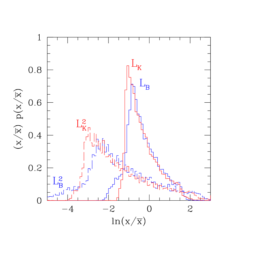
Figure 8: Distribution of normalized marks, $x/\bar{x}$, where $\bar{x}$ is the mean mark for $x=L_{B}$, $L_{B}^{2}$, $L_{K}$ and $L_{K}^{2}$. Notice that the distributions of normalized $L_{B}$ and $L_{K}$ are rather similar; nevertheless, the associated marked statistics shown in Figures 2 and 9 are very different.

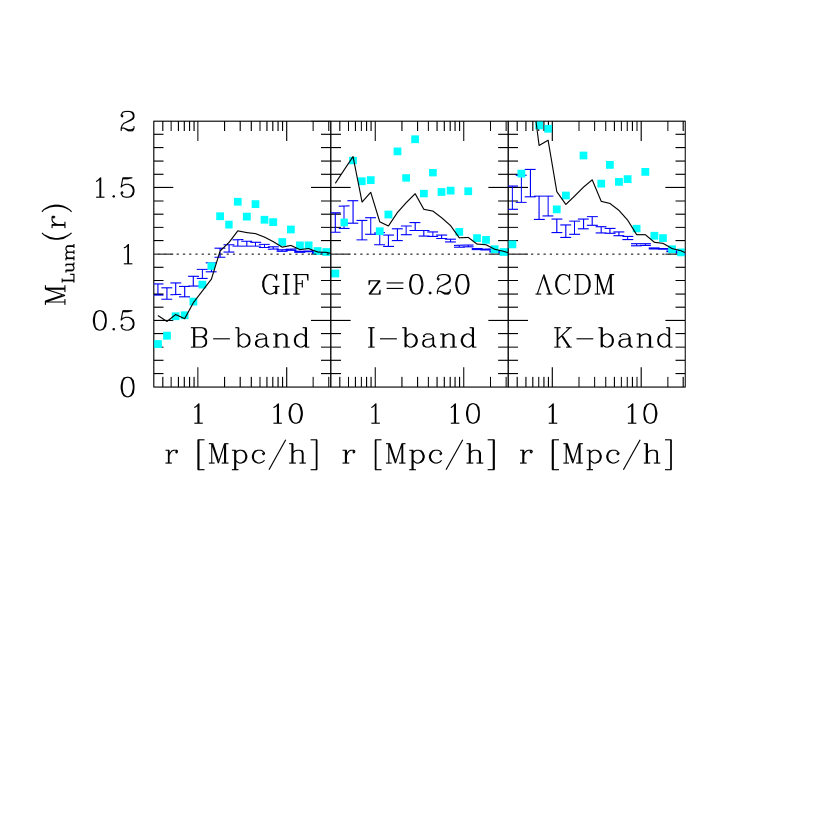
Figure 9: Comparison of statistic when normalized luminosity is the mark (error bars) and when the square of the luminosity (suitably normalized) is the mark. Curves show that $M_{L}^{2}(r)\sim M_{L^{2}}(r)$, with approximate equality on large scales where $M_{L}(r)\to 1$.

We remarked in Section 2.4 that monotonic rescaling of the marks may also be useful if one wishes to study marked statistics when the marks are not positive definite. A specific example is galaxy color (although it happens that the distribution of $V-I$ in the models we have studied in the previous section is positive definite, so that this was not an issue). We have studied the effect of rescaling from $V-I$ to $L_{I}/L_{V}\equiv 10^{-0.4(V-I)}$, with a curious result. Because one of the marks is a monotonic (in this case exponential) transformation of the other, it is natural to wonder if $M_{V-I}$ or $M_{L_{I}/L_{V}}$ shows a clearer signal. One might reasonably expect that the distribution of $V-I$ will have smaller tails than that of $L_{I}/L_{V}$. Since $M_{V-I}$ increases on small scales, one might expect this increase to be even more pronounced for $M_{L_{I}/L_{V}}$. On the other hand, since the precision of the measurement depends on the variance of the mark, one might expect $M_{L_{I}/L_{V}}$ to be the noisier measurement. However, what matters is not the distribution of the mark itself, but that of the mark normalized by its mean value. It happens that, upon normalizing by the mean of the rescaled mark, the distributions of $V-I$ and $L_{I}/L_{V}$ are almost indistinguishable! Hence, the resulting marked statistics are also almost indistinguishable.

It is possible to be more quantitative about this point. Figures 7 and 9 show that while the qualitative scale dependence of $(1+W)/(1+\xi)$ does not depend on rescaling, it does matter quantitatively. This raises the question of whether or not rescaling is advisable: if rescaling produces a marked statistic that differs more from unity than did the original mark, then perhaps rescaling is desirable. For instance, suppose one rescales to a distribution which has longer tails than the original [e.g., replace all marks $w$ with $\exp(w)$]. If $M(r)>1$ on small scales originally, then it is possible that after rescaling, $M(r)$ is even larger than before. To address whether this represents a real improvement in signal, one must also consider the precision with which the rescaled marked statistic can be measured. Thus, the relevant question is whether or not this rescaling has also increased the statistical significance of the difference from unity. Appendix A provides a discussion of the precision with which marked statistics can be estimated. Equation (A.2) there shows that the ratio of the rms value of the marked statistic to its mean value depends on the ratio of $\langle w_{1}^{2}w_{2}^{2}|r\rangle$ to $\langle w_{1}w_{2}|r\rangle^{2}$. Hence, rescaling is desirable if $W^{2}W^{2}/[WW]^{2}$ for the rescaled distribution is smaller than for the original distribution, or if the difference between the $WW/DD$ and unity, when expressed in units of the rms, $[1-DD/WW]/\sqrt{W^{2}W^{2}/[WW]^{2}-1/DD}$, is larger.

5 Discussion

Weighting galaxies by different marks (luminosity, star formation rate, etc.) yields datasets which are each biased differently relative to the underlying dark matter distribution. Study of marked statistics allows one to address issues such as: Which marks, if any, result in a weighting of the galaxy distribution which minimizes the bias relative to the dark matter? Over what redshift range is this mark the least biased? Cross correlations of marks also allow one to study, for example, if star formation rate, X-ray hardness or AGN activity are correlated with local density; if the color of a galaxy is correlated with the luminosity of its neighbour (the color of a galaxy is known to be strongly correlated with its own luminosity); and if luminosity dependent clustering is really due to morphological segregation.

A discussion of the bias and variance of estimators of marked statistics is provided in Appendix A. We also illustrated the use of marked statistics by showing how they behave in semi-analytic galaxy formation models. The models predict that the luminosity-weighted corrrelation function should depend strongly on waveband (Figure 2): close pairs should be more luminous than more widely separated pairs if the luminosity is measured at long wavelengths such as the $K$-band. If measured using the light from shorter wavelengths such as the $B$-band, the trend should be reversed: close pairs should be less luminous. If the models are correct, then luminosity marked correlations from the HST ACS and 2MASS should resemble the bottom left and right panels, respectively—they should be very different from each other.

Marked statistics also show that, in the models, close pairs of galaxies (separations smaller than $\sim 1$ Mpc) have redder colors and smaller star formation rates than more widely separated pairs (Figure 4), suggesting that objects in dense regions regions are redder and have smaller star formation rates. These trends are similar to the morphology-density (Dressler 1980) and star-formation rate-density relations (Lewis et al. 2002; Gomez et al. 2003). In addition, the stellar masses of objects in dense regions are larger, and the ratio of the typical stellar mass in dense regions to the average value is larger today than it was in the past (Figure 5).

We also showed that marked statistics provide simple tests of how correlations between observables depend on environment. As a specific example, the analysis of Section 2.6, when combined with the measurements of $M_{\rm stars}(r)$ and $M_{\rm L_{K}}$ (Figure 5) and the fact that $L_{K}\propto M_{\rm stars}$ (Figure 6) suggests that the mass-to-light ratio is larger in dense regions. It will be interesting to make similar measurements of marked statistics to determine whether or not other well-known correlations between galaxy observables correlate with environment. For instance, to test if the Fundamental Plane populated by early-type galaxy observables depends on environment, one would set $m=$ size and $w=$ the Fundamental Plane combination of surface brightness and velocity dispersion.

The virtue of marked statistics for identifying and quantifying trends with environment is that they do not rely on a specific choice of scale on which to define the larger scale environment, nor do they require a subjective division of galaxy environments into cluster and field. Indeed, marked correlations are particularly well-suited to studying correlations between galaxy properties and their environment, when the correlations are weak (Sheth & Tormen 2004). Because marked correlations do not pre-select a specific scale on which to study correlations with environment, they offer a powerful and complimentary approach to more traditional techniques which do require specific definitions of environment (e.g. Kauffmann et al. 2004; Hogg et al. 2005). Quantifying such correlations is interesting because galaxy formation models make specific predictions for environmental trends. This is because these models assume that galaxies form within dark matter halos, and the physical properties of galaxies are determined by the halos in which they form (White & Rees 1978; White & Frenk 1991). Therefore, the statistical properties of a given galaxy population are determined by the properties of the parent halo population.

The galaxy formation models of Kauffmann et al. (1999) and Cole et al. (2000) are based on this paradigm: they make rather similar assumptions for the complicated gastrophysics of galaxy formation. However, they make different assumptions about the resulting correlations with environment. In particular, because Kauffmann et al. (1999) use halo merger history trees from the simulations, their models include correlations between halo formation histories and environment. In contrast, Cole et al. (2000) use Monte Carlo merger histories, which explicitly ignore any correlation between halo formation and environment. Marked correlation functions provide an efficient way of quantifying the differences which result. In this regard, Skibba, Sheth & Connolly (2006) show how the observed luminosity dependence of clustering, when combined with a measurement of the luminosity weighted correlation function allows a sensitive test of the environmental dependence of galaxy clustering.

There are two main disadvantages associated with using marked statistics. First, although considerable effort has been spent in developing accurate models of how the galaxy correlation function depends on scale and time (see Cooray & Sheth 2002 for a review), there has been little parallel development of how marked correlations are expected to depend on scale and time. Hence, interpretting the measurements is not straightforward. However, this is beginning to change: Sheth, Abbas & Skibba (2004) show how to describe the weighted correlation function using the halo-model of large-scale structure, when galaxies are associated with halo substructure, and Sheth (2005) shows how the halo model can be used to describe all the marked statistics described here.

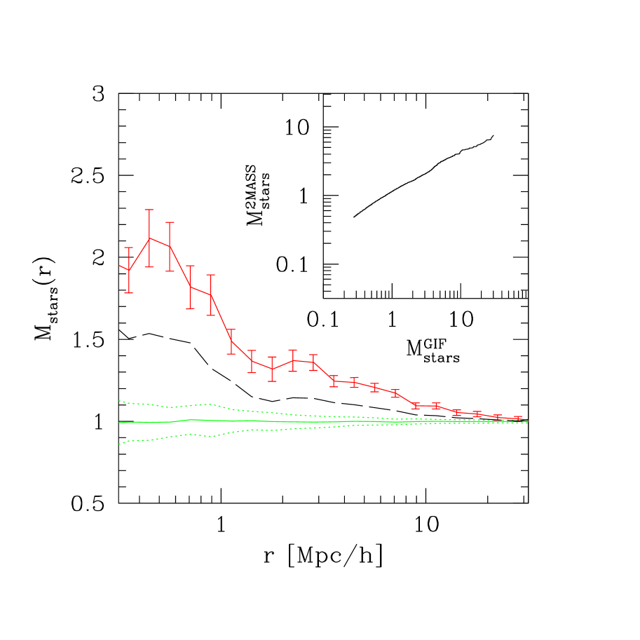
Figure 10: Comparison of statistic when normalized stellar mass is the mark. Top curve with error bars shows the result when the stellar mass is that from the GIF galaxy formation simulation, whereas dashed curve shows the statistic after applying a monotonic rescaling to the marks (shown as the inset in the upper right corner), so that they match the distribution of stellar masses reported by Cole et al. (2001).

Second, we have assumed that all analysis of marked statistics will be performed on volume limited catalogs. While direct measurement (using the estimator discussed here) of marked statistics in magnitude limited surveys is straightforward, interpretation is more complicated. For instance, one might use the halo-model framework to model the measurement. Development of a measurement algorithm which accounts for the effects of the magnitude limit is the subject of work in progress. There is, in addition, the inconvenience associated with the fact that our analysis assumes that the marks are positive definite, but arguments in Section 4 suggest that monotonic rescaling to a distribution which is positive definite will still yield useful results. Of course, all this assumes that the marks themselves have been accurately and precisely determined from the data.

Marked statistics are sensitive to the distribution of marks in the dataset. Because it is likely that the semi-analytic models will not match the observed distribution of galaxy properties (e.g., the current generation of models does not match the SDSS luminosity function, and the distribution of stellar masses does not match that infered from 2MASS), we envision that constraints on models will take the following form. If the models successfully describe the luminosity dependence of clustering, then they have successfully identified the halos in which galaxies form. Because the marked correlations are not changed in any essential way if the absolute values of the weights are altered without changing the rank ordering (Section 4), marked statistics provide a way of determining if, in addition to correctly identifying the halos in which galaxies form, the models also determine the correct rank ordering of galaxy properties within halos, if not their absolute values.

Figure 10 illustrates this procedure. It shows $(1+W)/(1+\xi)$ when stellar mass is the mark: the top curve with error bars shows the measurement in the GIF simulations (i.e., it is the same as in Figure 5), whereas the bottom dashed curve shows the result of rescaling the stellar masses so that they match the distribution reported by Cole et al. (2001) from their analysis of 2dF and 2MASS. To do this, we assumed that the marks in the GIF simulation are for the most massive galaxies in the simulation box. We then matched cumulative number densities, meaning that we worked our way down the GIF and Cole et al. stellar mass functions, assigning new masses to the semi-analytic galaxies until all 14665 objects had been assigned a 2dF-2MASS mass. Finally, we normalized these rescaled masses by their mean. The original and rescaled marks, normalized by their mean values, are shown in the inset in the top right corner of the Figure. This shows that, after rescaling, the marks span a smaller range of values around their mean value than they did originally. This has the effect of decreasing the amplitude of the rescaled marked statistic, but does not change the qualitative trend for close pairs to be more massive. More importantly, this illustrates that if the distribution of marks in the models does not match the data, then the marked statistic will also be discrepant.

The measurements presented here serve as benchmarks against which to compare measurements from data such as the SDSS (Abazajian et al. 2005). Measurements in the SDSS database using color, velocity dispersion, effective radius, morphology, star formation rate indicators, local density, and so on, as marks are underway (Skibba, Sheth & Connolly 2006). Comparison with predictions such as those described above will constrain the galaxy formation models.

Appendix A Error estimates

In what follows, we provide error estimates of the marked statistic most studied in the main text, the ratio of the weighted and unweighted correlation functions: $(1+W)/(1+\xi)$. We do this in two steps; the first assumes the marks are perfectly measured, and the second includes the effects of measurement errors. In either case, the analysis assumes that the mean mark can be reliably determined from the data. Our analysis follows that of Peebles (1980), Mo, Jing & Börner (1992), Landy & Szalay (1993) and Bernstein (1994).

A.1 An unbiased estimator

We estimate the statistic as $WW/DD$, where $WW$ is the sum over all pairs with separation $r$, weighting each member of the pair by its mark, and $DD$ is the total number of such pairs. In what follows, we assume that the marks have all been normalized by the mean mark, so that $DD$ really is the total number of pairs. (We discuss an alternative procedure, in which $DD$ is replaced by $W_{s}W_{s}$, which denotes the weighted pair counts in which the weights have been scrambled, shortly.) Let $\langle WW\rangle$ and $\langle DD\rangle$ denote the mean values of these statistics, where the mean is over an ensemble of realizations of the point process. The counts in any particular realization differ from this ensemble average value, so that

$$\Bigl{\langle}{WW\over DD}\Bigr{\rangle}={\langle WW\rangle\over\langle DD\rangle}\Bigl{\langle}{1+\omega\over 1+\delta}\Bigl{\rangle}\approx{\langle WW\rangle\over\langle DD\rangle}\,\Bigl{\langle}1+\omega-\delta-\omega\delta+\delta^{2}\Bigr{\rangle}.$$ (5)

The final expression follows from assuming $\delta\ll 1$ and keeping terms to second order. Now, $\langle\omega\rangle=0$ and $\langle\delta\rangle=0$ by definition, so the average of the ratio (the left hand side) equals the ratio of the averages (the right hand side) if $\langle\omega\delta\rangle=\langle\delta^{2}\rangle$. We can estimate these terms as follows. Let

$$\Bigl{\langle}DD\Bigr{\rangle}=\sum_{i<j}n_{i}n_{j}\,\Theta_{ij}(r)=U_{2}(r)$$ (6)

and

$$\Bigl{\langle}WW\Bigr{\rangle}=\sum_{i<j}w_{i}w_{j}\,\Theta_{ij}(r)=\Bigl{\langle}w_{1}w_{2}|r\Bigr{\rangle}\,U_{2}(r),$$ (7)

where $U_{2}(r)$ is proportional to the total number of pairs, $N(N-1)/2$, times a geometrical factor, $G_{2}(r)$, which represents the fraction of these pairs which have separation $r$, given the survey geometry (see, e.g., Landy & Szalay 1993). Then

$${\langle{DD\cdot DD}\rangle\over\langle DD\rangle\langle DD\rangle} = 1+\Bigl{\langle}\delta^{2}\Bigr{\rangle}$$ (8)

$$= {\sum_{i<j}n_{i}n_{j}\,\Theta_{ij}(r)\sum_{k<l}n_{k}n_{l}\,\Theta_{kl}(r)\over U_{2}(r)^{2}}$$

$$= {U_{4}(r)+U_{3}(r)+U_{2}(r)\over U_{2}(r)^{2}},$$

where $U_{4}(r)\equiv N(N-1)(N-2)(N-3)/4\,G^{2}_{2}(r)$, and $U_{3}(r)\equiv N(N-1)(N-2)\,G_{3}(r)$ are products of the total number of quadruples and triples times geometrical factors, defined similarly to $U_{2}(r)$. Similarly,

$${\langle{WW\cdot DD}\rangle\over\langle WW\rangle\langle DD\rangle} = 1+\Bigl{\langle}\omega\delta\Bigr{\rangle}$$ (9)

$$= {\sum_{i<j}w_{i}w_{j}\,\Theta_{ij}(r)\sum_{k<l}n_{k}n_{l}\,\Theta_{kl}(r)\over\langle w_{1}w_{2}|r\rangle\,U_{2}(r)^{2}}$$

$$= {\langle w_{1}w_{2}|r\rangle\,U_{4}(r)+\langle w_{1}w_{2}|r\rangle\,U_{3}(r)+\langle w_{1}w_{2}|r\rangle\,U_{2}(r)\over\langle w_{1}w_{2}|r\rangle\,U_{2}(r)^{2}}$$

$$= 1+\Bigl{\langle}\delta^{2}\Bigr{\rangle}.$$

Thus,

$$\Bigl{\langle}{WW\over DD}\Bigr{\rangle}={\langle WW\rangle\over\langle DD\rangle};$$ (10)

this estimator is unbiased.

Notice that if we had not normalized the marks by their mean value, but had replaced $DD$ by $W_{s}W_{s}$, then the estimator would be unbiased provided we treated each of the $W_{s}$ terms as being drawn from a different realization of the scrambled marks. This is because terms of the form $\langle w^{2}\rangle$ in the expression for $\langle W_{s}W_{s}\cdot W_{s}W_{s}\rangle$ lead to a bias. Thus, the weights in the numerator of $WW/W_{s}W_{s}$ must be treated differently from those in the denominator, making the notation somewhat confusing. This is why we prefer to use $WW/DD$ (with the understanding that the weights have been normalized by their mean value), rather than $WW/W_{s}W_{s}$ as our estimator.

A.2 Variance within a bin

The variance of the estimator is

$${\rm Var}\left[{WW\over DD}\right] = {\langle WW\rangle^{2}\over\langle DD\rangle^{2}}\Bigl{\langle}{(1+\omega)^{2}\over(1+\delta)^{2}}\Bigl{\rangle}-\Bigl{\langle}{WW\over DD}\Bigr{\rangle}^{2}$$ (11)

$$= {\langle WW\rangle^{2}\over\langle DD\rangle^{2}}\Bigl{\langle}1+\omega^{2}-4\omega\delta+3\delta^{2}\Bigr{\rangle}-\Bigl{\langle}{WW\over DD}\Bigr{\rangle}^{2}$$

$$= {\langle WW\rangle^{2}\over\langle DD\rangle^{2}}\,\Bigl{\langle}\omega^{2}-\delta^{2}\Bigr{\rangle}$$

where the final expression uses the fact that $\langle\omega\delta\rangle=\langle\delta^{2}\rangle$.

The sum in quadrature of the variances of $WW$ and $DD$ is proportional to $\langle\omega^{2}\rangle+\langle\delta^{2}\rangle$. Notice that the expression above scales as the difference of these two terms rather than than the sum, so it can be substantially smaller. This reflects the fact that, if $WW$ for a given realization of the point process is larger than the ensemble mean, it may simply be large because $DD$ is also large (i.e., there were more pairs). As a result, fluctuations in $WW$ and $DD$ are correlated. The estimate of the true variance above accounts for this correlation.

To see what it is, note that

$${\langle{WW\cdot WW}\rangle\over\langle WW\rangle\langle WW\rangle}=1+\Bigl{\langle}\omega^{2}\Bigr{\rangle}$$ (12)

$$= {\sum_{i<j}w_{i}w_{j}\,\Theta_{ij}(r)\sum_{k<l}w_{k}w_{l}\,\Theta_{kl}(r)\over\langle w_{1}w_{2}|r\rangle^{2}\,U_{2}(r)^{2}}$$

$$\approx {U_{4}(r)\over U^{2}_{2}(r)}+{\langle w_{1}^{2}w_{2}w_{3}|r\rangle\,U_{3}(r)+\langle w_{1}^{2}w_{2}^{2}|r\rangle\,U_{2}(r)\over\langle w_{1}w_{2}|r\rangle^{2}\,U_{2}(r)^{2}}.$$

so the ratio of the variance to the square of the mean is

$${{\rm Var}[WW/DD]\over\langle WW/DD\rangle^{2}} \approx {\langle w_{1}^{2}w_{2}w_{3}|r\rangle-\langle w_{1}w_{2}|r\rangle^{2}\over\langle w_{1}w_{2}|r\rangle^{2}}\,{U_{3}(r)\over U^{2}_{2}(r)}$$ (13)

$$+{\langle w_{1}^{2}w_{2}^{2}|r\rangle-\langle w_{1}w_{2}|r\rangle^{2}\over\langle w_{1}w_{2}|r\rangle^{2}}\,{U_{2}(r)\over U_{2}(r)^{2}}.$$

On large scales, where correlations tend to be weak, $U_{3}\approx N_{\rm gal}\,(\bar{n}\,{\rm d}V)^{2}(1+\xi)^{3}/2$ and $U_{2}\approx N_{\rm gal}\,\bar{n}\,{\rm d}V\,(1+\xi)/2$ so $U_{3}/U_{2}^{2}\approx 2(1+\xi)/N_{\rm gal}$. Hence, the first term in the expression above scales as $1/N_{\rm gal}$. The second term scales inversely with the number of pairs, so, for a sufficiently large survey, the first term dominates on large scales, whereas the second term dominates on small scales.

The second term scales sensibly as the inverse of the pair counts, times a term which resembles a variance of mark pairs. It is useful to think of this term as

$$\left[{\langle w_{1}^{2}w_{2}^{2}|r\rangle\over\langle w_{1}w_{2}|r\rangle^{2}}-1\right]\Bigl{/}U_{2}(r)=\left[{M_{w^{2}}(r)\over M^{2}_{w}(r)}{\langle w^{2}\rangle^{2}\over\langle w\rangle^{4}}-1\right]\Bigl{/}U_{2}(r);$$

here $M_{w^{2}}(r)$ denotes the statistic when the mark is the square of the weight, rather than the weight itself. Thus, this term can be estimated directly from the data as $W^{2}W^{2}/[WW]^{2}-1/DD$. Notice that if $M_{w^{2}}=M_{w}^{2}$, then this term can be written in terms of the variances of $w$ and $w^{2}$, so the only scale dependence comes from the factor of $U_{2}$. Figure 9 in the main text shows that this approximation may not be wildly-off in astrophysical datasets.

The first term is more problematic; its presence suggests that a better estimator than $WW/DD$ for our marked statistic can be found, just as a better estimator than $DD/RR$ can be found for the unweighted statistic $1+\xi$. Writing down this alternative estimator is beyond the scope of the present paper. However, to see the effect of this extra term, suppose that there are no correlations, either between the points, or between the marks. This is not an unreasonable assumption on the large scales where the first term is expected to dominate. In this limit,

$${{\rm Var}[WW/DD]\over\langle WW/DD\rangle^{2}}\approx\left[{\langle w^{2}\rangle\over\langle w\rangle^{2}}-1\right]{2\over N_{\rm gal}}.$$ (14)

The form of this expression suggests that the variance should be well approximated by adding

$$\left[{\langle w^{2}|r\rangle\over\langle w_{1}w_{2}|r\rangle}-1\right]{2\,[1+\xi(r)]\over N_{\rm gal}}$$ (15)

to $W^{2}W^{2}/[WW]^{2}-1/DD$. Figure 3 in the main text illustrates how these two terms are expected to contribute to the error budget in typical astrophysical datasets.

The analysis so far does not account for the possibility that, if the dataset is small, then the estimated pair counts are not from a fair sample, so they will be biased. This introduces additional terms into the error budget, which can be estimated by relatively straightforward but tedious extension of the analysis in Landy & Szalay (1993). Also absent from this error budget is the fact that small datasets may not provide accurate measurements of the mean mark. Since our analysis assumes that all marks have been normalized by this mean measured in the dataset, this introduces an additional source of error. A more detailed account of these two additional sources of error will be presented elsewhere. Note that astrophysical datasets are now becoming sufficiently large that small sample issues are less likely to be a serious concern, so the estimates here should be reasonably accurate.

A.3 Covariance between bins

In this case, we are interested in

$${\rm cov}\left[{W_{1}W_{1}\over D_{1}D_{1}}{W_{2}W_{2}\over D_{2}D_{2}}\right] = {\langle W_{1}W_{1}\rangle\langle W_{2}W_{2}\rangle\over\langle D_{1}D_{1}\rangle\langle D_{2}D_{2}\rangle}\,\Bigl{\langle}\delta_{1}\delta_{2}+\omega_{1}\omega_{2}$$ (16)

$$\qquad\qquad-\omega_{1}\delta_{2}-\omega_{2}\delta_{1}\Bigr{\rangle}$$

where we have used the fact that

$$\left\langle{W_{1}W_{1}\over D_{1}D_{1}}{W_{2}W_{2}\over D_{2}D_{2}}\right\rangle = {\langle W_{1}W_{1}\rangle\langle W_{2}W_{2}\rangle\over\langle D_{1}D_{1}\rangle\langle D_{2}D_{2}\rangle}\,\Bigl{\langle}1+\delta_{1}^{2}+\delta_{2}^{2}+\delta_{1}\delta_{2}$$

$$-\omega_{1}\delta_{1}-\omega_{2}\delta_{2}+\omega_{1}\omega_{2}-\omega_{1}\delta_{2}-\omega_{2}\delta_{1}\Bigr{\rangle}$$

and we have set $\langle\omega_{i}\delta_{i}\rangle=\langle\delta_{i}^{2}\rangle$. Hence, the covariance depends on

$${\langle D_{i}D_{i}\cdot D_{j}D_{j}\rangle\over\langle D_{i}D_{i}\rangle\langle D_{j}D_{j}\rangle}=1+\Bigl{\langle}\delta_{i}\delta_{j}\Bigr{\rangle}=1+{U_{3}(r_{i},r_{j})\over U_{2}(r_{i})\,U_{2}(r_{j})},$$ (17)

$${\langle W_{i}W_{i}\cdot D_{j}D_{j}\rangle\over\langle W_{i}W_{i}\rangle\langle D_{j}D_{j}\rangle}=1+\Bigl{\langle}w_{i}\delta_{j}\Bigr{\rangle}=1+\Bigl{\langle}\delta_{i}\delta_{j}\Bigr{\rangle},$$ (18)

and

$${\langle W_{i}W_{i}\cdot W_{j}W_{j}\rangle\over\langle W_{i}W_{i}\rangle\langle W_{j}W_{j}\rangle} = 1+\Bigl{\langle}w_{i}w_{j}\Bigr{\rangle}$$ (19)

$$= 1+W_{3}(r_{i},r_{j})\,{U_{3}(r_{i},r_{j})\over U_{2}(r_{i})\,U_{2}(r_{j})},$$

with

$$W_{3}(r_{i},r_{j})={\langle w_{1}^{2}w_{2}w_{3}|r_{i},r_{j}\rangle\over\langle w_{1}w_{2}|r_{i}\rangle\langle w_{1}w_{3}|r_{j}\rangle}-1.$$ (20)

A.4 Measurement errors

The analysis above assumes the marks are perfectly measured. If, instead, the marks are imprecisely measured, but, while imprecise, are unbiased, and if the measurement error is not correlated with spatial position, then the previous expressions hold with $\langle\omega^{2}\rangle\to\langle\omega^{2}+\epsilon^{2}\rangle$ where $\langle\epsilon^{2}\rangle$ denotes the variance of the error on mark. Hence, the measurement errors do not bias the marked statistic, but they do increase Var$[WW/DD]$, thus decreasing the precision of the measurement. Of course, if the measurement of the marks themselves is systematically biased, then the marked statistics will also be biased.

References

- [1] Abazajian K., et al., 2005, AJ, 129, 1755
- [2] Beisbart C., Kerscher M., 2000, ApJ, 545, 6
- [3] Benoist C., Cappi A., da Costa L. N., Maurogordato S., Bouchet F., Schaeffer R., 1999, ApJ, 514, 563
- [4] Bernstein G., 1994, ApJ, 424, 569
- [5] Cole S., Norberg, P, Baugh C. M., Frenk C. S., et al., 2001, MNRAS, 326, 255
- [6] Cole S., Lacey C., Baugh C. M., Frenk C. S., 2000, MNRAS, 321, 559
- [7] Colless M., et al., 2001, MNRAS, 328, 1039
- [8] Connolly A. J., Szalay A. S., Bershady M. A., Kinney A. L., Calzetti D., 1995, AJ, 110(3), 1071
- [9] Connolly A. J., Scranton R., Johnston D., et al., 2002, ApJ, 579, 42
- [10] Cooray A., Sheth R. K., 2002, Phys. Rep., 372, 1
- [11] Dressler A., 1980, ApJ, 236, 351
- [12] Evrard A. E., MacFarland T. J., Couchman H. M. P., Colberg J. M, et al., 2002, ApJ, 573, 7
- [13] Faber S. M., Jackson R. E., 1976, ApJ, 204, 668
- [14] Gomez P., et al., 2003, ApJ, 584, 210
- [15] Hamilton A. J. S., 1988, ApJL, 331, L59
- [16] A. J. S. Hamilton, M. Tegmark, 2002, MNRAS, 330, 506
- [17] Kauffmann G. A. M., Colberg J. M., Diaferio A., White S. D. M., 1999, MNRAS, 303, 188
- [18] Kauffmann G. A. M., White S. D. M., Heckman T. M., Ménard B., Brinchmann J., Charlot S., Tremonti C., Brinkmann J., 2004, MNRAS, 353, 713
- [19] Lahav O., Naim A., Sodré L., Storrie-Lombardi M. C., 1996, MNRAS, 283, 207
- [20] Landy S. D., Szalay A. S., 1993, ApJ, 412, 64
- [21] Lewis I., et al., 2002, MNRAS, 334, 673
- [22] Maddox S. J., Efstathiou G., Sutherland W. J., Loveday J., 1990, MNRAS, 242, 43P
- [23] Mo H. J., Börner G., Zhou Y., 1989, AA, 221, 191
- [24] Mo H. J., Jing Y. P., Börner G., 1992, ApJ, 392, 452
- [25] Mo H. J., White S. D. M., 1996, MNRAS, 282, 347
- [26] Moore A., Connolly A. J., Genovese C., Gray A., Grone L., Kanidoris N., Nichol R. C., Schneider J., Szalay A. S., Szapudi I., Wasserman L., in Mining the Sky, Proceedings of the MPA/ESO/MPE Workshop. Eds. A. J. Banday, S. Zaroubi & M. Bartelmann. Heidelberg: Springer Verlag, p.71 (2001)
- [27] Norberg P., Baugh C. M., Hawkins E., Maddox S. J., et al., 2002, MNRAS, 332, 827
- [28] Percival W. P., et al., 2001, MNRAS, 327, 1297
- [29] P. J. E. Peebles (1980), The Large Scale Structure of the Universe. Princeton.
- [30] Sheth R. K., 2005, MNRAS, ???, ???
- [31] Sheth R. K., Lemson G., 1999, MNRAS, 304, 767
- [32] Sheth R.K., Abbas U., Skibba R.A., in Diaferio A., ed, Proc. IAU Coll. 195, Outskirts of galaxy clusters: intense life in the suburbs, CUP, Cambridge, p. 349
- [33] Skibba R., Sheth R. K., Connolly A. J., 2006, MNRAS, submitted (astro-ph/0512???)
- [34] Somerville R. S., Primack J. R., 1999, MNRAS, 310, 1087
- [35] Springel V., et al., 2005, Nature, 435, 629
- [36] Storrie-Lombardi M. S., Lahav O., Sodré L., Storrie-Lombardi L. J., 1992, MNRAS, 259, 8P
- [37] Stoyan D., 1984, Math. Nachr., 116, 197
- [38] Stoyan D., Stoyan H., 1994, Fractals, Random Shapes, and Point Fields. Wiley & Sons, Chichester
- [39] Totsuji H., Kihara T., 1969, PASJ, 21, 221
- [40] Tully R. B., Fisher J. R., 1977, A&A, 54(3), 661
- [41] White S. D. M., Rees M. J., 1978, MNRAS, 183, 341
- [42] White S. D. M., Frenk C. S., 1991, ApJ, 379, 52
- [43] Willmer C. N. A., da Costa L. N., Pellegrini P. S., 1998, AJ, 115(3), 869
- [44] Zehavi I., Blanton M. R., Frieman J. A., Weinberg D. H., et al., 2002, ApJ, 571, 172
- [45] Zehavi I., Blanton M. R., Frieman J. A., Weinberg D. H., et al., 2005, ApJ, 630, 1