The halo-model description of marked statistics

Abstract

Marked statistics allow sensitive tests of how galaxy properties correlate with environment, as well as of how correlations between galaxy properties are affected by environment. A halo-model description of marked correlations is developed, which incorporates the effects which arise from the facts that typical galaxy marks (e.g., luminosity, color, star formation rate, stellar mass) depend on the mass of the parent halo, and that massive haloes extend to larger radii and populate denser regions. Comparison with measured marked statistics in semi-analytic galaxy formation models shows good agreement on scales smaller than a Megaparsec, and excellent agreement on larger scales. The halo-model description shows clearly that the behaviour of some low-order marked statistics on these scales encodes information about the mean galaxy mark as a function of halo mass, but is insensitive to mark-gradients within haloes. Higher-order statistics encode information about higher order moments of the distribution of marks within haloes. This information is obtained without ever having to identify haloes or clusters in the galaxy distribution. On scales smaller than a Megaparsec, the halo-model calculation shows that marked statistics allow sensitive tests of whether or not central galaxies in haloes are a special population. A prescription for including more general mark-gradients in the halo-model description is also provided. The formalism developed here is particularly well-suited to interpretation of marked statistics in astrophysical datasets, because it is phrased in the same language that is currently used to interpret more standard measures of galaxy clustering.

1 Introduction

Almost all clustering analyses to date treat galaxies as points without attributes. However, galaxies have luminosities, sizes, shapes, velocity dispersions, star formation rates, etc. Recent work (Hamilton 1988; Norberg et al. 2002; Zehavi et al. 2005) has begun to study how galaxy correlations depend on luminosity and color—the more luminous galaxies are more strongly clustered, and red galaxies tend to cluster more strongly than blue. However, the quality of the data is now sufficiently good that one can imagine measuring, not just galaxy clustering as a function of galaxy attribute, but the spatial correlations of the attributes themselves. That is to say, rather than measuring clustering as a function of luminosity, one can now measure the clustering of luminosity (or of color, star-formation rate etc.).

Börner, Mo & Zhao (1989) were among early pioneers, studying the correlation functions of galaxies with different weightings according to luminosity and mass. Although also discussed by Peebles (1980), this sort of approach has been formalized under the framework of marked point processes (e.g. Stoyan 1984; Stoyan & Stoyan 1994). Marked statistics have recently been applied to astrophysical datasets by Beisbart & Kerscher (2000), Beisbart, Kerscher & Mecke (2002), Gottlöber et al. (2002) and Faltenbacher et al. (2002).

Marked statistics provide a useful framework for describing point processes in which the points have attributes or weights. They are particularly well-suited to identifying and quantifying correlations between galaxy properties (luminosities, colors,, stellar masses, star formation rates) and their environments (e.g. Sheth, Connolly & Skibba 2005), particularly when such correlations are weak (Sheth & Tormen 2004). The halo model (reviewed in Cooray & Sheth 2002) is the framework within which traditional (i.e. unmarked) measurements of galaxy clustering are currently interpretted (e.g., Magliochetti & Porciani 2003, Mo et al. 2004; Zehavi et al. 2005; Collister & Lahav 2005). This paper develops the halo-model description of marked statistics.

Section 2 defines a number of marked statistics. Section 3 provides a halo model calculation of these marked statistics, under the assumption that marks do not correlate with spatial position within haloes. The analysis extends ideas presented in Sheth, Abbas & Skibba (2004). It then compares the halo-model description with measurements in simulations. Section 4 shows how the halo-model description can be extended to allow for correlations between marks and position within halo—mark gradients. It pays special attention to the case in which the central object in a halo is different from all the others. The analysis shows how the halo model can be used to test simple physical models of why galaxy properties correlate with environment. On larger scales, the halo-model description of marked statistics shows that they can be thought of as being linearly biased versions of unweighted statistics—this is the subject of Section 5. A final section discusses how the methods presented here provide the basis for interpretating measurements of marked statistics which can be made with databases currently available. It also shows how marked statistics can be used to interpret measurements which indicate that correlations between galaxy properties (e.g., the correlation between stellar mass and $K$-band luminosity) also correlate with environment. An Appendix illustrates some of the key ideas using a fully analytic toy model.

2 Marked statistics

In what follows, a mark is a weight or attribute associated with each point in a point process. To make the discussion less abstract, we will often use astrophysical terms to illustrate our arguments. Thus, a point process is a galaxy catalog, and a mark can be any observable property associated with a galaxy, such as luminosity, color, velocity dispersion, size, star formation rate, etc. Marked statistics measure the clustering of marks. Since the positions at which the marks are measured may themselves be clustered, marked statistics are defined in a way which accounts for this.

For example, let $\bar{\rho}$ denote the mean density of particles, and let $\bar{w}$ denote the mean mark, averaged over all particles. Now consider a particle with mark larger than this mean value. Are the particles neighbouring it also likely to have larger marks? One way to quantify this is to compute the ratio of the mean mark to $\bar{w}$ of pairs of particles as a function of pair separation. The typical number of pairs at separation $r$ is $\bar{\rho}^{2}[1+\xi(r)]$, where $\xi$ is the two point correlation function. Therefore, the mean mark is

$${\cal M}_{1}(r) = {\sum[w({{\mbox{\boldmath$x$}}})+w({{\mbox{\boldmath$y$}}})]\,{\cal I}(|{{\mbox{\boldmath$x$}}}-{{\mbox{\boldmath$y$}}}|-r)\over 2\bar{w}\ \sum{\cal I}(|{{\mbox{\boldmath$x$}}}-{{\mbox{\boldmath$y$}}}|-r)}$$ (1)

$$= {\sum[w({{\mbox{\boldmath$x$}}})+w({{\mbox{\boldmath$y$}}})]\,{\cal I}(|{{\mbox{\boldmath$x$}}}-{{\mbox{\boldmath$y$}}}|-r)\over 2\bar{w}\ \bar{\rho}^{2}[1+\xi(r)]},$$

where ${\cal I}(x)=0$ unless $x=0$, and the sum is over all galaxy pairs. We have divided by $\bar{w}$, so ${\cal M}_{1}(r)=1$ for all $r$ if there are no correlations between marks. Analogously, the $n$th-order mark is defined by

$${\cal M}_{n}(r)={\sum[w({{\mbox{\boldmath$x$}}})+w({{\mbox{\boldmath$y$}}})]^{n}\,{\cal I}(|{{\mbox{\boldmath$x$}}}-{{\mbox{\boldmath$y$}}}|-r)\over(2\bar{w})^{n}\ \bar{\rho}^{2}[1+\xi(r)]}.$$ (2)

For what follows, it is also useful to define

$${\cal C}_{n}(r)={\sum[w({{\mbox{\boldmath$x$}}})-w({{\mbox{\boldmath$y$}}})]^{n}\,{\cal I}(|{{\mbox{\boldmath$x$}}}-{{\mbox{\boldmath$y$}}}|-r)\over(2\bar{w})^{n}\ \bar{\rho}^{2}[1+\xi(r)]}.$$ (3)

It is sufficiently straightforward to generalize these concepts of $n$-th order marks from pairs to $N$-tuples that we have not written the expressions explicitly.

In what follows, we will mainly study the cases when $n=1$ and 2. In this regard, it is helpful to re-write ${\cal M}_{2}$ as

$${\cal M}_{2}(r) = {\sum[w({{\mbox{\boldmath$x$}}})-w({{\mbox{\boldmath$y$}}})]^{2}\ {\cal I}(|{{\mbox{\boldmath$x$}}}-{{\mbox{\boldmath$y$}}}|-r)\over(2\bar{w})^{2}\ \bar{\rho}^{2}[1+\xi(r)]}$$ (4)

$$\quad+\quad{\sum w({{\mbox{\boldmath$x$}}})w({{\mbox{\boldmath$y$}}})\,{\cal I}(|{{\mbox{\boldmath$x$}}}-{{\mbox{\boldmath$y$}}}|-r)\over\bar{w}^{2}\ \bar{\rho}^{2}[1+\xi(r)]}.$$

The second term involves a similar sum to that which defines $1+\xi$, except that now each particle of the pair contributes a weight $w$. Thus, the second term can be thought of as a ‘weighted’ correlation function. If we write it as $[1+W(r)]/[1+\xi(r)]$ then

$${\cal M}_{2}(r)={\cal C}_{2}(r)+{1+W(r)\over 1+\xi(r)}.$$ (5)

When $n=2$, it is perhaps more intuitive to study the mark variance and covariance, defined by

$${\rm var}(r)={\cal M}_{2}(r)-{\cal M}_{1}^{2}(r)+{\cal C}_{2}(r)$$ (6)

and

$${\rm cov}(r)={\cal M}_{2}(r)-{\cal M}_{1}^{2}(r)-{\cal C}_{2}(r).$$ (7)

To help build intuition, it is perhaps useful to consider how one might estimate these marked statistics in a data set. Consider the quantity $1+\xi(r)$ which appears in the denominator of all the expressions above. A common estimator for it is to simply sum the number of data pairs with separation $r$ in the point distribution and divide it by the number of pairs of similar separation in a random distribution. The suggestive notation for this estimator is $DD/RR$. Now consider the quantity $(1+W)/(1+\xi)$. Similarly suggestive notation for the estimator of $1+W(r)$ is $WW/RR$. However, since we are interested in the ratio of these two terms, the appropriate estimator is $WW/DD$. Note that $DD$ is precisely the term in the sum in the denominator of equation (1). Since $WW/DD$ is simply the average over all pairs in the sample of the product of the weights, it can be estimated without explicitly constructing a random catalog, and without explicitly worrying about the survey geometry. Similarly simple estimators for the other marked statistics defined above can also be constructed (e.g., ${\cal M}_{1}(r)$ can be estimated as $WD/DD$), making them far less time-consuming to estimate than the usual unweighted statistics such as $\xi$.

3 The halo model description

This section describes how the marked statistics defined above can be written in the language of the halo model. The analysis below complements and extends ideas in Sheth, Abbas & Skibba (2004).

In the halo model (Cooray & Sheth 2002, and references therein), the nonlinear density field is assumed to be made up of dense objects called haloes. At any given time, haloes of different masses all have the same density (they are all approximately two hundred times denser than the background). All mass is in such haloes, and so all galaxies are also associated with haloes.

In this description, the two-point correlation function $\xi(r)$ is determined by the sum of two types of galaxy pairs: pairs in the same halo, and pairs in separate haloes. Since the radius of a typical halo at $z=0$ is less than a Mpc, the one-halo term is negligible on scales larger than a few Mpc. On the small scales where the one-halo term dominates, the shape of $\xi(r)$ is determined by how halo density profiles depend on halo mass, and on how halo abundances depend on mass; on larger scales, $\xi(r)$ is less sensitive to the shapes of halo profiles, and more sensitive to the clustering of the haloes themselves.

For this description, it may help to think of the galaxy distribution as a density field, in which case

$${\cal M}_{n}(r)={\Bigl{\langle}[w({{\mbox{\boldmath$x$}}})+w({{\mbox{\boldmath$x$}}}+{{\mbox{\boldmath$r$}}})]^{n}\,\rho({{\mbox{\boldmath$x$}}})\rho({{\mbox{\boldmath$x$}}}+{{\mbox{\boldmath$r$}}})\Bigr{\rangle}\over(2\bar{w})^{n}\,\Bigl{\langle}\rho({{\mbox{\boldmath$x$}}})\rho({{\mbox{\boldmath$x$}}}+{{\mbox{\boldmath$r$}}})\Bigr{\rangle}},$$ (8)

where the angle brackets denote averages over all space.

3.1 Unweighted statistics

In the halo model, all mass is bound up in dark matter haloes which have a range of masses. Hence, the density of galaxies is

$$\bar{n}_{\rm gal}=\int dm\,{dn(m)\over dm}\,g_{1}(m),$$ (9)

where $dn(m)/dm$ denotes the number density of haloes of mass $m$, and

$$g_{n}(m)\equiv\sum_{N}N(N-1)...(N-n+1)\,p(N|m)$$ (10)

is the $n$-th factorial moment of the distribution $p(N|m)$ of galaxies in $m$-haloes. If $p(N|m)$ follows a Poisson distribution, then $g_{n}(m)=g_{1}^{n}(m)$.

The correlation function is the Fourier transform of the power spectrum $P(k)$:

$$\xi(r)=\int{dk\over k}\,{k^{3}P(k)\over 2\pi^{2}}\,{\sin kr\over kr}.$$ (11)

In the halo model, $P(k)$ is written as the sum of two terms: one that arises from particles within the same halo and dominates on small scales (the 1-halo term), and the other from particles in different haloes which dominates on larger scales (the 2-halo term). Namely,

$$P(k)=P_{1h}(k)+P_{2h}(k),$$ (12)

where

$$P_{1h}(k) = \int dm\,{dn(m)\over dm}\,{g_{2}(m)\,u(k|m)^{2}\over\bar{n}_{\rm gal}^{2}},$$

$${P_{2h}(k)\over P_{\rm Lin}(k)} = \left[\int dm\,{dn(m)\over dm}\,{g_{1}(m)\,u(k|m)\over\bar{n}_{\rm gal}}\,b(m)\right]^{2}.$$

Here $u(k|m)$ is the Fourier transform of the halo density profile divided by $m$, $b(m)$ is the bias factor which describes the strength of halo clustering, and $P_{\rm Lin}(k)$ is the power spectrum of the mass in linear theory. When explicit calculations are made, we assume that the density profiles of haloes have the form described by Navarro et al. (1996), and that halo abundances and clustering are described by the parameterization of Sheth & Tormen (1999).

3.2 Marked statistics when marks are independent of position within halo

Now consider the weights. Let $p({{\mbox{\boldmath$w$}}}|N,{{\mbox{\boldmath$r$}}},m)\,d{{\mbox{\boldmath$w$}}}$ denote the probability that the $N$ galaxies at positions $({{\mbox{\boldmath$r$}}}_{1},\ldots,{{\mbox{\boldmath$r$}}}_{N})$ in an $m$-halo have weights ${{\mbox{\boldmath$w$}}}=(w_{1},\ldots,w_{N})$.

As our simplest model, we will consider the case in which the weights do not depend on position within the halo. If, in addition, these weights are independent, then $p({{\mbox{\boldmath$w$}}}|N,m)\,d{{\mbox{\boldmath$w$}}}=\prod_{i=1}^{N}p(w_{i}|N,m)\,dw_{i}$. If the distribution of weights depends on $m$ but is independent of $N$, then this simplifies further to

$$p({{\mbox{\boldmath$w$}}}|N,m)\,d{{\mbox{\boldmath$w$}}}=\prod_{i=1}^{N}p(w_{i}|m)\,dw_{i}.$$ (13)

Note that this model assumes that the weight associated with one galaxy is independent of the others within a halo, but that the distribution of weights depends on the mass of the parent halo. Later we will compare this model with one in which the distribution of weights depends on distance from the centre of the parent halo, but is otherwise independent of the other objects in the halo.

The mean weight associated with galaxies in $m$-haloes is

$$\langle w|m\rangle=\prod_{i=1}^{N}\int dw_{i}\,p(w_{i}|m){\sum_{i=1}^{N}w_{i}\over N}=\int dw\,p(w|m)\,w.$$ (14)

The mean weight averaged over all haloes is

$$\bar{w}=\int dm\,{dn(m)\over dm}\,{\langle w|m\rangle\,g_{1}(m)\over\bar{n}_{\rm gal}}\,.$$ (15)

If we define

$$p(w)=\int dm\,{dn(m)\over dm}\,{g_{1}(m)\over\bar{n}_{\rm gal}}\,p(w|m)$$ (16)

then

$$\langle w^{n}\rangle = \int dw\,p(w)\,w^{n}$$ (17)

$$= \int dm\,{dn(m)\over dm}\,{g_{1}(m)\over\bar{n}_{\rm gal}}\int dw\,p(w|m)\,w^{n}$$

$$= \int dm\,{dn(m)\over dm}\,{g_{1}(m)\over\bar{n}_{\rm gal}}\,\langle w^{n}|m\rangle.$$

The marked statistics defined in the previous section require averages over particle pairs. So, for instance,

$${\cal M}_{1}(r)={1+{\cal W}_{1}(r)\over 1+\xi(r)}$$ (18)

where ${\cal W}_{1}(r)$ is the Fourier transform of

$${\cal W}_{1}(k)={\cal W}_{1}^{1h}(k)+{\cal W}_{1}^{2h}(k),$$ (19)

with

$${\cal W}_{1}^{1h}(k) = \int dm\,{dn(m)\over dm}{\langle w|m\rangle\over\bar{w}}\,{g_{2}(m)\,|u(k|m)|^{2}\over\bar{n}_{\rm gal}^{2}},$$

$${{\cal W}_{1}^{2h}(k)\over P_{\rm Lin}(k)} = \Biggl{[}\int dm\,{dn(m)\over dm}\,b(m){\langle w|m\rangle\over\bar{w}}\,{g_{1}(m)\over\bar{n}_{\rm gal}}\,u(k|m)\Biggr{]}$$

$$\times\Biggl{[}\int dm\,{dn(m)\over dm}\,b(m){g_{1}(m)\over\bar{n}_{\rm gal}}\,u(k|m)\Biggr{]}$$

and $\xi(r)$ was defined earlier. Note the similarity between the integrals which define $P_{1h}$ and $P_{2h}$, and those for ${\cal W}_{1}^{1h}$ and ${\cal W}_{1}^{2h}$.

Similarly, we can write

$${\cal M}_{2}(r)={[1+\langle w^{2}\rangle/\bar{w}^{2}]/2+{\cal W}_{2}(r)\over 1+\xi(r)}$$ (20)

where ${\cal W}_{2}(r)$ is the Fourier transform of

$${\cal W}_{2}(k)={\cal W}_{2}^{1h}(k)+{\cal W}_{2}^{2h}(k),$$ (21)

with

$${\cal W}_{2}^{1h}(k) = \int dm\,{dn(m)\over dm}{\langle w^{2}|m\rangle+\langle w|m\rangle^{2}\over 2\bar{w}^{2}}$$

$$\qquad\qquad\times\quad{g_{2}(m)\,|u(k|m)|^{2}\over\bar{n}_{\rm gal}^{2}}\,$$

$${{\cal W}_{2}^{2h}(k)\over P_{\rm Lin}(k)} = \Biggl{[}\int dm\,{dn(m)\over dm}\,b(m){\langle w|m\rangle\over\sqrt{2}\bar{w}}\,{g_{1}(m)\over\bar{n}_{\rm gal}}\,u(k|m)\Biggr{]}^{2}$$

$$+\Biggl{[}\int dm\,{dn(m)\over dm}\,b(m){\langle w^{2}|m\rangle\over 2\bar{w}^{2}}\,{g_{1}(m)\over\bar{n}_{\rm gal}}\,u(k|m)\Biggr{]}$$

$$\quad\times\quad\Biggl{[}\int dm\,{dn(m)\over dm}\,b(m){g_{1}(m)\over\bar{n}_{\rm gal}}\,u(k|m)\Biggr{]},$$

If we define the variance of the weights in $m$-haloes as

$$V^{2}(w|m)\equiv\langle w^{2}|m\rangle-\langle w|m\rangle^{2},$$ (22)

and set

$$V^{2}(w)\equiv\langle w^{2}\rangle-\langle w\rangle^{2},$$ (23)

then

$${\cal W}_{2}^{1h}(k) = \int dm\,{dn(m)\over dm}\,{\langle w|m\rangle^{2}\over\bar{w}^{2}}\,{g_{2}(m)\,|u(k|m)|^{2}\over\bar{n}_{\rm gal}^{2}}\,$$

$$+\int dm\,{dn(m)\over dm}{V^{2}(w|m)\over 2\bar{w}^{2}}{g_{2}(m)\,|u(k|m)|^{2}\over\bar{n}_{\rm gal}^{2}}\,$$

$${{\cal W}_{2}^{2h}(k)\over P_{\rm Lin}(k)} = \Biggl{[}\int dm\,{dn(m)\over dm}\,b(m){\langle w|m\rangle\over\bar{w}}\,{g_{1}(m)\over\bar{n}_{\rm gal}}\,u(k|m)\Biggr{]}^{2}$$

$$+\Biggl{[}\int dm\,{dn(m)\over dm}\,b(m){\langle w^{2}|m\rangle\over 2\bar{w}^{2}}\,{g_{1}(m)\over\bar{n}_{\rm gal}}\,u(k|m)\Biggr{]}$$

$$\quad\times\quad\Biggl{[}\int dm\,{dn(m)\over dm}\,b(m){g_{1}(m)\over\bar{n}_{\rm gal}}\,u(k|m)\Biggr{]}$$

$$-\Biggl{[}\int dm\,{dn(m)\over dm}\,b(m){\langle w|m\rangle\over\sqrt{2}\bar{w}}\,{g_{1}(m)\over\bar{n}_{\rm gal}}\,u(k|m)\Biggr{]}^{2}.$$

Let $W(k)$ denote the sum of the first term of ${\cal W}_{2}^{1h}$ with the first term of ${\cal W}_{2}^{2h}$. Then the Fourier transform of $W(k)$ is the weighted correlation function $W(r)$ (e.g. insert this expression in equation 20 and compare with equation 5). These expressions show that ${\cal M}_{1}(r)$ and the weighted correlation function $W(r)$ encode information about the first moment of $p(w|m)$; information about the scatter around $\langle w|m\rangle$ comes from ${\cal M}_{2}(r)$.

If the distribution of weights, $p(w|m)$, does not depend on $m$, then $\langle w|m\rangle=\bar{w}$, so ${\cal W}_{1}(k)=P(k)$, and ${\cal M}_{1}(r)=1$. Similarly, ${\cal W}_{2}(k)=[(1+\langle w^{2}\rangle/\bar{w}^{2})/2]\,P(k)$, and so ${\cal M}_{2}(r)=(1+\langle w^{2}\rangle/\bar{w}^{2})/2$. This is sensible: if the distribution of weights is independent of $m$, then ${\cal M}_{2}(r)$ is simply the average value of a quantity which is the square of the sum of two random variates divided by $4\bar{w}^{2}$. Thus, if $p(w|m)$ does not depend on $m$, the marked correlations are constants, independent of scale, and they have the values associated with truly independent marks.

However, the expressions above show that marked statistics can have non-trivial scale-dependence if $p(w|m)$ depends on $m$, even though galaxy marks do not depend on position with the parent halo, and the mark of one galaxy is otherwise independent of the marks associated with the others. That is, galaxy marks are only correlated with the masses of their parent haloes; all other correlations between galaxy marks are a consequence of this correlation. In such a model, the small-scale dependence of marked correlations is a consequence of the fact that the size of a halo depends on its mass. On larger scales, the dominant cause of nontrivial scale-dependence of the weighted correlation function is that the spatial distribution of haloes is mass-dependent.

Notice that the two halo contribution to ${\cal M}_{1}(r)$ and to the weighted correlation function $W(r)$ depend on the combination $g_{1}(m)\,\langle w|m\rangle$; this quantity is the sum of the marks in a halo, averaged over all halos of mass $m$—the mean total mark in $m$-haloes. This shows that the large scale behaviour of these two statistics encodes information about how this quantity depends on halo mass. Note that this information is provided without ever actually dividing the galaxy distribution up into clusters. Furthermore, if the number of galaxies in a halo follows a Poisson distribution, then $g_{2}(m)=g_{1}(m)^{2}$, and the one-halo contribution to $W(r)$ encodes information about the square of this quantity.

3.3 Comparison with simulations

Before building a more sophisticated model, it is worth checking how well this simple description fares when compared with marked statistics measured in models of galaxy formation. The GIF semi-analytic galaxy formation models of Kauffmann et al. (1999) provide a useful testbed for the halo model description developed above. Measurements of marked statistics for a variety of marks in these simulations have been presented in Sheth, Connolly & Skibba (2005). We study some of them here. In all cases, the measurements are for a sample of galaxies which contain more than $2\times 10^{10}h^{-1}M_{\odot}$ in stars at $z=0.2$ in a flat $\Lambda$CDM cosmology with $(\Omega_{0},h,\sigma_{8})=(0.3,0.7,0.9)$. The redshift was chosen to approximately match the median redshift of the 2dFGRS (Colless et al. 2001) and SDSS (York et al. 2000; Abazajian et al. 2003) surveys. The mock galaxy catalog contains about 14,665 objects in a cubical comoving volume $141h^{-1}$Mpc on a side.

The halo-model calculation requires knowledge of the first and second factorial moments of the galaxy counts in haloes. Figure 1 shows how these quantities scale with halo mass. The smooth curves show

$$g_{1}(m) = \left({m_{11}\over 250}\right){\rm e}^{-10/m_{11}}+1-{\rm e}^{-(m_{11}/15)^{6}}$$

$$\sqrt{g_{2}(m)} = \left({m_{11}\over 250}\right){\rm e}^{-1/m_{11}}+0.9\,\exp\left(-{m_{11}\over 1000}-{100\over m_{11}}\right),$$

where $m_{11}$ denotes the halo mass in units of $10^{11}h^{-1}M_{\odot}$.

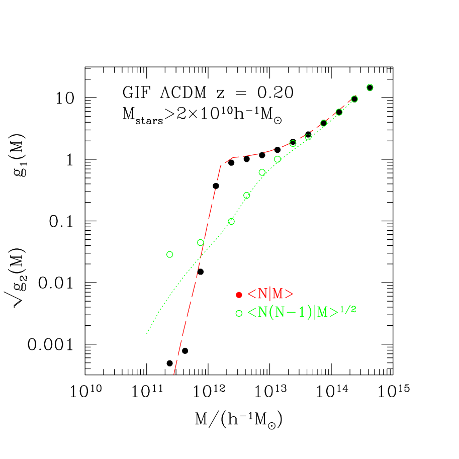
Figure 1: First and second factorial moments of the distribution of the number of galaxies with stellar mass greater than $2\times 10^{10}h^{-1}M_{\odot}$ in haloes of mass $M$ in the GIF $\Lambda$CDM semi-analytic galaxy formation models at $z=0.2$.

In addition, calculation of marked statistics requires how the mean weight or mark depends on halo mass. Figure 2 shows this mass-dependence for a variety of weights: open triangles, filled triangles, squares, crosses, circles and stars show how the mean $L_{B}$, $L_{V}$, $L_{I}$, $L_{K}$, stellar mass, and star formation rate depend on halo mass. Most of these marks are steeply increasing functions of halo mass, at least in the range $2\times 10^{12}\leq M/h^{-1}M_{\odot}\leq 2\times 10^{13}$. At larger masses, the mean luminosity-weights are approximately constant, but depend strongly on waveband—on average, galaxies in massive haloes are more luminous than average, although this over-luminosity is larger in the redder bands. For a given weight, these trends with mass give rise to nontrivial scale dependence of the marked statistics. The different mass dependence of the weights makes the marked statistics depend on the type of mark.

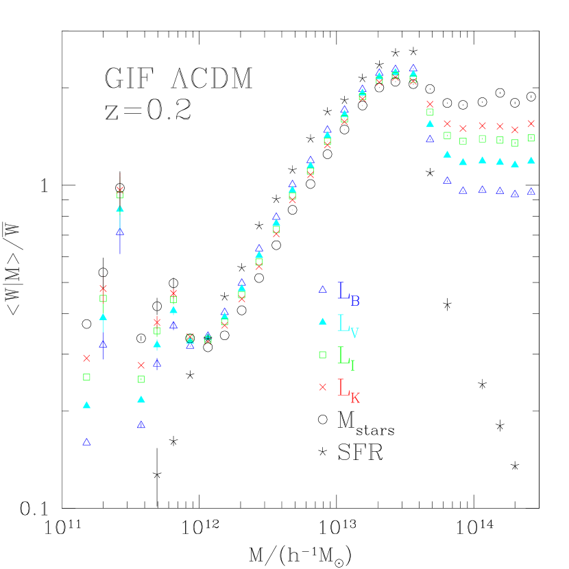
Figure 2: Mean mark as a function of parent halo mass in the GIF semi-analytic galaxy formation models at $z=0.2$, for a variety of marks. While differences between the marks are relatively small in the range $10^{12}\leq M/h^{-1}M_{\odot}\leq 10^{13}$, more massive galaxies are more luminous than the mean in the redder bands. The mass dependence of any given mark gives rise to nontrivial scale dependence of the associated marked statistics.

Figure 3 illustrates these differences using the luminosities in the reddest and bluest bands as the marks. Results for the two marked statistics which depend only on the mean mark within haloes are shown: the symbols in the top panels show ${\cal M}_{1}(r)$ in the simulations when the $B$- (left) and $K$-band (right) luminosities are used as the mark; symbols in the bottom panels show the ratio of the weighted and unweighted pair counts $(1+W)/(1+\xi)$.

In all panels, the dotted lines show the result of randomizing the marks, and then repeating the measurement of the statistic one hundred times. The mean of these random realizations is shown (it is virtually indistinguishable from unity) bracketed by the rms scatter around it. This gives a rough indication of the typical uncertainty on the measurement (this estimated uncertainty assumes uncorrelated marks, so it is almost certainly an underestimate of the true error on the measurement).

Note the non-trivial scale dependence of the statistics in each panel, and note that the scale-dependence is very different in the two bands. Close pairs tend to be more luminous than average in $K$, but less luminous than average in $B$.

The smooth dashed curves in the different panels show the result of inserting $g_{1}(m)$, $g_{2}(m)$ and $\langle W|m\rangle$ from the simulations (c.f. Figures 1 and 2) in the halo model formulae given earlier. (In practice, we approximate the two-halo terms using the simpler expressions given in Section 5.) Recall that all scale dependence in these calculations is the result of the fact that massive haloes extend to larger radii and populate denser regions, and that the mean weight depends on halo mass. There are no additional environmental effects, and there are no correlations between luminosity and position with the halo. Comparison with the symbols shows excellent agreement on scales larger than $2h^{-1}$Mpc, suggesting that the analytic calculation has captured the essence of the physics at large separations. On smaller scales, however, there are differences, particularly for the weighted correlation functions shown in the bottom panels. The agreement on the larger scales which are dominated by the two-halo term is reassuring, because it suggests that modification to the one-halo term is all that is necessary to describe the statistics.

Figure 4 shows similar results, but now when the star formation rate is used as the mark. As when the luminosity was the mark, the halo model calculation provides a reasonable description of the marked statistics on scales larger than a few Mpc, but it significantly over-predicts the signal on small scales. In the next section, we argue that most of this discrepancy arises from the fact that, although the model allows for the possibility that marks may depend on halo mass, it does not allow marks to depend on position within a halo. Thus, comparison of the model curves with the measurements provides some indication of the importance of such mark-gradients. Evidently, such gradients only matter on small scales; this is sensible, since one does not expect the detailed distribution of marks within a halo to affect measurements on scales which are significantly larger than that of a typical halo.

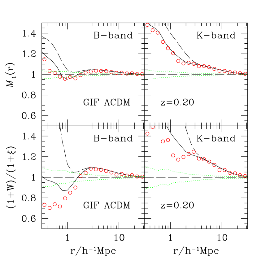
Figure 3: Marked statistics in which $B$- and $K$-band luminosities were used as the mark. Symbols show measurements in the GIF semi-analytic galaxy formation models, and dotted curves show an estimate of the uncertainty on the measurement. Dashed curves show the halo-model calculation developed earlier, in which there is no distinction between the central galaxy and all the others in a halo. Solid curves show the halo-model calculation described in Section 4.1, in which central galaxies are special.

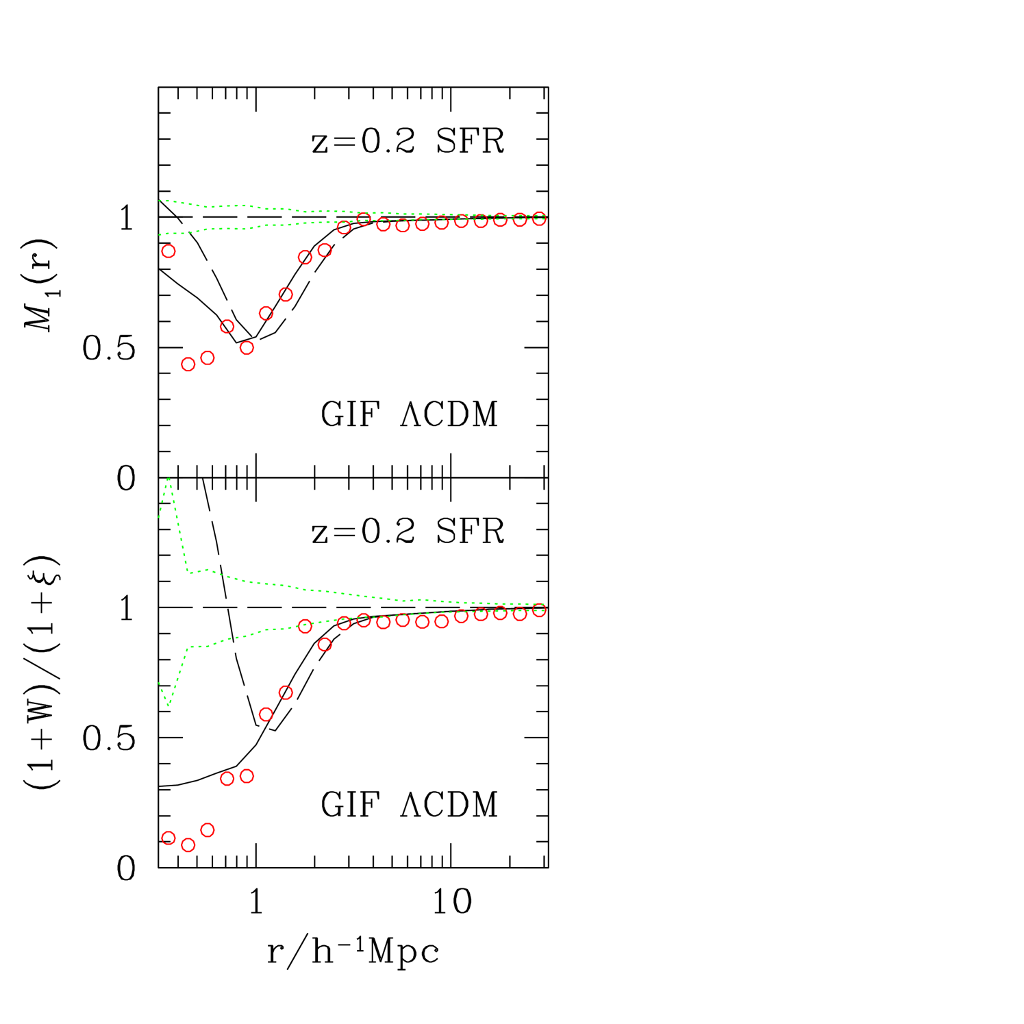
Figure 4: Marked statistics in which star formation rate was used as the mark. Symbols show measurements in the GIF semi-analytic galaxy formation models, and dotted curves show an estimate of the uncertainty on the measurement. Dashed curves show the halo-model calculation developed earlier, and solid curves show the halo-model calculation developed in Section 4.1.

The next section shows how the halo model can be extended to include mark-gradients, thus allowing one to address the question of what causes these gradients. In particular, we show that allowing the central object in a halo to be different from all the others accounts for most of the discrepancy on small scales.

4 Marked statistics when marks depend on position within halo

This section provides two simple parametrizations of the effects of a correlation between galaxy mark and position within the halo. In the first model, this correlation is particularly simple: the central galaxy in a halo is supposed to be different from all the others, but, other than this, all the previous assumptions about the independence of marks apply. This case, while simple, is a standard assumption in semi-analytic and SPH-based galaxy formation models (e.g. Kauffmann et al. 1999; Zheng et al. 2005). It is also precisely the approximation currently used to interpret measurements of the luminosity dependence of galaxy clustering. The second model allows for more sophisticated correlations between galaxy mark and position within the halo; it may be useful in studies where the mark is galaxy color, since redder galaxies in a halo are expected to be more centrally concentrated than the bluer ones.

However, in neither model is the mark of one galaxy within a halo physically correlated with that of another: the correlation is purely statistical. For instance, Zheng et al. (2005) find that, in their semi-analytic models, there is a weak correlation between the number and luminosity of satellite galaxies in less massive haloes and the luminosity of the central galaxy: both are smaller if the central galaxy is more luminous. Such a correlation is not present in the models developed below. One signature of such a physical correlation would be a successful description of ${\cal M}_{1}(r)$ even on small scales, but gross discrepancies between model and measured $(1+W)/(1+\xi)$. Since we see discrepancies in both the upper and lower panels of Figures 3 and 4, this is less of an immediate concern. In any case, accounting for this correlation is more complicated, and will be reported elsewhere.

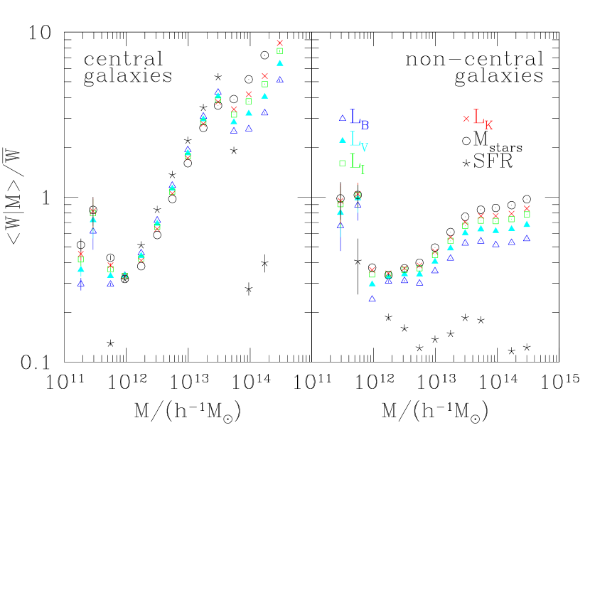
Figure 5: Mean mark as a function of parent halo mass in the GIF semi-analytic galaxy formation models at $z=0.2$, for a variety of marks. Panel on the left shows the mean mark for the central galaxy in a halo, and panel on the right shows the mean mark for the other galaxies. It is interesting to compare both these panels with Figure 2.

4.1 The centre-satellite model

Figure 2 shows how the mean mark depends on halo mass. This mean value was computed by averaging over all the galaxies in a halo, whatever their location within it. However, in the GIF models, the central galaxy in a halo is very different from the others. To illustrate, Figure 5 shows the same marks as in Figure 2, but now the marks associated with the central galaxy (left panel) are shown separately from those associated with the other galaxies (right panel). Clearly, the mass-dependence of the marks is very different in the two cases. The halo model calculations of the previous section showed that mass dependence of any given mark gives rise to nontrivial scale dependence of the associated marked statistics. Hence, it is possible that the failure of the halo model calculation on small scales (in the previous section) was due to the neglect of this difference between central and satellite objects. In this respect, the model must be extended to allow for a correlation between the value of the mark and its location.

To include this effect, assume that haloes which host galaxies host one and only one central galaxy, and possibly many non-central galaxies. We will sometimes refer to these other galaxies as satellites. Let $g_{1}^{\rm cen}(m)$ denote the fraction of $m$-haloes which host a central galaxy, and let $g_{n}^{\rm sat}(m)$ denote the $n$th factorial moment of the distribution of the number of satellites in a halo. Further, define

$$g_{1}^{\rm cs}(k|m)\equiv g_{1}^{\rm cen}(m)+g_{1}^{\rm sat}(m)\,u(k|m)\\$$ (24)

and

$$g_{1}^{\rm wcs}(k|m)\equiv{g_{1}^{\rm cen}(m)\,\langle w_{\rm cen}|m\rangle+g_{1}^{\rm sat}(m)\,\langle w_{\rm sat}|m\rangle\,u(k|m)\over\bar{w}};$$ (25)

these are the analogues of the mean number times density profile, and mark-weighted number times density profile. Currently popular (centre plus Poisson satellite) models (e.g. Kravtsov et al. 2004) have $g_{1}^{\rm cen}(m)=1$ for $m$ greater than some minimum mass, $g_{1}^{\rm cen}=0$ for smaller $m$, $g_{1}^{\rm sat}(m)=0$ if $g_{1}(m)<1$, and $g_{2}^{\rm sat}(m)=[g_{1}^{\rm sat}(m)]^{2}$.

Since there can only be one central galaxy, the unweighted correlation function $\xi(r)$ is the Fourier transform of the sum of

$$P_{1h}(k) = \int dm\,{dn(m)\over dm}\,\Biggl{[}{2\,g_{1}^{\rm cen}(m)g_{1}^{\rm sat}(m)\,u(k|m)\over\bar{n}_{\rm gal}^{2}}$$

$$\qquad\qquad\qquad\qquad+\ {g_{2}^{\rm sat}(m)\,u(k|m)^{2}\over\bar{n}_{\rm gal}^{2}}\Biggr{]},$$

$${P_{2h}(k)\over P_{\rm Lin}(k)} = \left[\int dm\,{dn(m)\over dm}\,{g_{1}^{\rm cs}(k|m)\over\bar{n}_{\rm gal}}\,b(m)\right]^{2}.$$

The first term in $P_{1h}$ represents the contribution from centre-satellite–, and the second from satellite-satellite–pairs. (The density run of central galaxies around their host haloes is a delta-function.)

Similarly, the halo model estimate of ${\cal M}_{1}(r)$ requires evaluation of

$${\cal W}_{1}^{1h}(k) = \int dm\,{dn(m)\over dm}{\langle w_{\rm cen}|m\rangle+\langle w_{\rm sat}|m\rangle\over 2\bar{w}}$$

$$\qquad\qquad\times\ {2\,g_{1}^{\rm cen}(m)g_{1}^{\rm sat}(m)\,u(k|m)\over\bar{n}_{\rm gal}^{2}}$$

$$+\ \int dm\,{dn(m)\over dm}{\langle w_{\rm sat}|m\rangle\over\bar{w}}{g_{2}^{\rm sat}(m)\,u(k|m)^{2}\over\bar{n}_{\rm gal}^{2}},$$

$${{\cal W}_{1}^{2h}(k)\over P_{\rm Lin}(k)} = \Biggl{[}\int dm\,{dn(m)\over dm}\,b(m){g_{1}^{\rm wcs}(k|m)\over\bar{n}_{\rm gal}}\Biggr{]}$$

$$\times\Biggl{[}\int dm\,{dn(m)\over dm}\,b(m)\,{g_{1}^{\rm cs}(k|m)\over\bar{n}_{\rm gal}}\Biggr{]}.$$

And the Fourier transform of the weighted correlation function becomes

$$W_{1h}(k) = \int dm\,{dn(m)\over dm}{\langle w_{\rm cen}|m\rangle\over\bar{w}}{\langle w_{\rm sat}|m\rangle\over\bar{w}}$$

$$\qquad\times\ {2\,g_{1}^{\rm cen}(m)g_{1}^{\rm sat}(m)\,u(k|m)\over\bar{n}_{\rm gal}^{2}}$$

$$+\int dm\,{dn(m)\over dm}{\langle w_{\rm sat}|m\rangle^{2}\over\bar{w}^{2}}{g_{2}^{\rm sat}(m)\,u(k|m)^{2}\over\bar{n}_{\rm gal}^{2}},$$

$${W_{2h}(k)\over P_{\rm Lin}(k)} = \Biggl{[}\int dm\,{dn(m)\over dm}\,b(m)\,{g_{1}^{\rm wcs}(k|m)\over\bar{n}_{\rm gal}}\,\Biggr{]}^{2}.$$

The solid curves in Figures 3 and 4 show these halo model calculations; they are in substantially better agreement with the measurements than the dashed curves. (In practice, we approximate the two-halo terms by the simpler expressions given in Section 5.)

It is easy to see why this happens. Consider, for example, the $K$-band luminosity. Figure 5 shows that the central object is usually substantially more luminous than the satellites, especially at higher masses. Moreover, the satellites are also less luminous than when we assign them weights in which the central object is not treated as special, as in Figure 2. When the central object is special, then pairs with separations of order the diameter of a typical halo will be dominated by the satellite-satellite term. Since this has smaller weights than when the centre was not special, the resulting values of ${\cal M}_{1}$ and $(1+W)/(1+\xi)$ are smaller. Similar consideration of the differences between mean satellite weights when the central object is and is not special explains the qualitative differences between the solid and dashed curves in Figures 3 and 4.

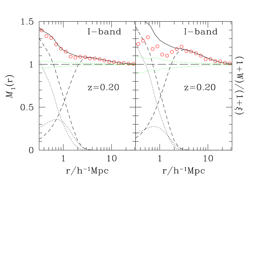
Figure 6: Marked statistics in which $I$-band luminosities were used as the mark. Symbols show measurements in the GIF semi-analytic galaxy formation models, and dotted curves show an estimate of the uncertainty on the measurement. Solid curves show the full halo-model calculation developed in Section 4.1, in which central galaxies are special. The two dashed curves in each panel show the one- and two-halo contributions to the statistic, and the dotted curves show the centre-satellite and the satellite-satellite contributions to the one-halo term. The centre-satellite term dominates on the smallest scales.

Figure 6 provides an explicit demonstration of the relative roles played by the various terms in the model when the mark is $I$-band luminosity. The panel on the left shows results for ${\cal M}_{1}$ and the panel on the right shows $(1+W)/(1+\xi)$. The symbols show the measured values, and the band around unity traced out by the dotted lines shows an estimate of the uncertainty on the measurements calculated by randomizing the marks (as for the previous figures). The solid curve shows the full marked correlation; the two short dashed curves show the one- and two-halo contributions, and the two dotted curves show the centre-satellite (dominates on small scales) and satellite-satellite contributions to the one-halo term.

It is worth emphasizing that, in Figures 3 and 4, the mean mark in $m$-haloes is the same function of $m$ for both the solid and the dashed curves—the only difference is in the physical interpretation of this mean mark. The solid curves represent a model in which the central galaxy in a halo is different from all the others, whereas the dashed curves show the expected marked statistics if the central galaxy were not special. Thus, our analysis shows that marked statistics are well-suited to discriminating between different physical models of galaxy properties.

The previous plot shows how different physical models of the marks within halos result in different marked statistics. For completeness, Figure 7 shows how the dependence of the mean mark on halo mass affects the statistic. From bottom to top, the different curves show the relative contribution from halos with masses greater than $10^{14}h^{-1}M_{\odot}$, $10^{13}h^{-1}M_{\odot}$, and $10^{12.5}h^{-1}M_{\odot}$ (meaning that, for the $1+\xi$ term in the denominator, the integrals were performed over the entire range of halo masses, but that they were restricted to masses greater than these values when the numerator was computed). The full signal (solid curves) is very well approximated by the signal from halos more massive than $10^{12}h^{-1}M_{\odot}$, as one might expect from a glance at Figure 1. These curves indicate that the small scale signal is dominated by halos with masses around $10^{13}h^{-1}M_{\odot}$ and greater, but that on larger scales, the contribution from less massive halos is more significant than that of more massive halos.

Figure 7: Marked statistics in which $I$-band luminosities were used as the mark, shown as a function of the halo mass range which contributes. Symbols show the same measured values as in the previous figure, and solid curves show the same full halo-model calculation. The three dashed curves in each panel show the fractional contributions of the term in the numerator of the halo-model expression for the marked correlation function from halos more massive than $10^{14}h^{-1}M_{\odot}$ (bottom), $10^{13}h^{-1}M_{\odot}$ (middle), and $10^{12.5}h^{-1}M_{\odot}$ (top).

4.2 A more general case

This section provides a simple parametrization of the effects of a correlation between galaxy mark and position within the halo. We continue to assume that there are otherwise no correlations between the marks of one galaxy and another. Specifically, assume that there is a deterministic relation between distance from the halo centre and the value of the mark: $w(r|m)$. (For instance, suppose some galaxy property depends on the local density or velocity dispersion within the parent halo. In reality there is almost certainly scatter in this relation; we think of $w(r|m)$ as an average value). Then

$$p(w|m)\,{\rm d}w=p(r|m)\,{\rm d}r=4\pi r^{2}\,{\rho(r|m)\over m}\,{\rm d}r,$$ (26)

for some monotonic relation $w(r|m)$, and so

$$\langle w|m\rangle=\int{\rm d}w\,p(w|m)\,w=\int{\rm d}r\,p(r|m)\,w(r|m).$$ (27)

If we define

$$w(k|m)\equiv{\int{\rm d}r\,4\pi r^{2}\,w(r|m)\,\rho(r|m)\,\sin(kr)/kr\over\int{\rm d}r\,4\pi r^{2}\,w(r|m)\,\rho(r|m)},$$ (28)

then this quantity is the normalized Fourier transform of the weighted density profile.

Note that although there is no scatter in the marks at fixed $r$, there is scatter in the marks at fixed pair separation (the two members of a pair of fixed separation can come from different distances from the halo center). Thus, in this model, the variance in weights at fixed pair separation is non-trivial.

The marked statistic ${\cal M}_{1}(r)$ is now given by terms like

$${\cal W}_{1}^{1h}(k) = \int dm\,{dn(m)\over dm}{\langle w|m\rangle\over\bar{w}}\,{g_{2}(m)\,w(k|m)u(k|m)\over\bar{n}_{\rm gal}^{2}},$$

$${{\cal W}_{1}^{2h}(k)\over P_{\rm Lin}(k)} = \Biggl{[}\int dm\,{dn(m)\over dm}\,b(m){\langle w|m\rangle\over\bar{w}}\,{g_{1}(m)\over\bar{n}_{\rm gal}}\,w(k|m)\Biggr{]}$$

$$\times\Biggl{[}\int dm\,{dn(m)\over dm}\,b(m){g_{1}(m)\over\bar{n}_{\rm gal}}\,u(k|m)\Biggr{]};$$

in effect, the fact that the weight now has a profile means that one must replace one power of $u(k|m)$ with $w(k|m)$. Similarly, $W(k)$, the Fourier transform of the weighted correlation function, becomes $W_{1h}(k)+W_{2h}(k)$ where

$$W_{1h}(k) = \int dm\,{dn(m)\over dm}{\langle w|m\rangle^{2}\over\bar{w}^{2}}\,{g_{2}(m)\,|w(k|m)|^{2}\over\bar{n}_{\rm gal}^{2}},$$

$${W_{2h}(k)\over P_{\rm Lin}(k)} = \Biggl{[}\int dm\,{dn(m)\over dm}\,b(m){\langle w|m\rangle\over\bar{w}}\,{g_{1}(m)\over\bar{n}_{\rm gal}}\,w(k|m)\Biggr{]}^{2}.$$

In this case, both powers of $u(k|m)$ have been replaced.

Note in particular that the effect of mark-gradients is expected to be more dramatic for $(1+W)/(1+\xi)$ than it is for ${\cal M}_{1}$: $W_{1h}$ requires two powers of $u(k|m)\to w(k|m)$, whereas ${\cal W}_{1h}$ only requires one. Thus, the analysis above indicates that incorporating weight-gradients in the halo-model description is relatively straightforward. Appendix A illustrates these effects using a fully analytic toy model of the gradients. We expect this model to be useful for studying color gradients in clusters.

If there are true correlations between the weights of one galaxy and others in the same halo (such as the weak correlation reported by Zheng et al. 2005), then the expression for $W_{1h}(k)$ becomes more complicated still. The analysis above suggests that $|w(k|m)|^{2}$ in the integrand for $W_{1h}$ should be replaced with a term which accounts for the correlation between the marks, as well as the shape of the density profile; this is the subject of work in progess.

5 Biasing on large scales

On scales which are larger than the diameter of a typical halo, the marked statistics above are dominated by the contribution from pairs in separate haloes. In this limit, the scale dependence of marked statistics is simply related to the shape of the linear theory power spectrum. To see why, consider the unweighted correlation function $\xi(r)$, the weighted correlation function $W(r)$ and the additive marked statistic ${\cal M}_{1}(r)$. On large scales, the Fourier transforms of halo profiles $u(k|m)\to 1$. Hence, $g_{1}^{\rm cs}(k|m)\to g_{1}^{\rm cen}+g_{1}^{\rm sat}\equiv g_{1}(m)$ and $g_{1}^{\rm wcs}(k|m)\to g_{1}(m)\langle w|m\rangle/\bar{w}$. If we define

$$b_{\rm gal}\equiv\int dm\,{dn(m)\over dm}\,{g_{1}(m)\over\bar{n}_{\rm gal}}\,b(m)$$ (29)

and

$$b_{w1}\equiv\int dm\,{dn(m)\over dm}\,{g_{1}(m)\over\bar{n}_{\rm gal}}\,{\langle w|m\rangle\over\bar{w}}\,b(m),$$ (30)

then

$$P_{2h}(k) \approx b_{\rm gal}^{2}\,P_{\rm Lin}(k),$$ (31)

$${\cal W}_{1}^{2h}(k) \approx b_{\rm gal}\,b_{w1}\,P_{\rm Lin}(k),\qquad{\rm and}$$ (32)

$$W_{2h}(k) \approx b_{w1}^{2}\,P_{\rm Lin}(k),$$ (33)

on large scales. Thus, suitably defined combinations of $\xi$, $W$ and ${\cal M}_{1}$ provide measurements of $b_{w1}/b_{\rm gal}$.

In practice, measurement of $\xi$ requires use of a random catalog as well as knowledge of the survey boundary, whereas measurements of marked statistics do not (c.f. discussion at the end of Section 2). Hence, the most straightforward measurement of $b_{w1}/b_{\rm gal}$ comes from using the fact that, on large scales

$${[1+W(r)]/[1+\xi(r)]-1\over{\cal M}_{1}(r)-1}\approx 1+{b_{w1}\over b_{\rm gal}}.$$ (34)

The previous sections showed that, on large scales, the halo model calculation is in excellent agreement with the simulations. Hence, our analysis shows that marked correlations allow a simple measurement of this ratio. It is also straightforward to estimate the relative bias factors associated with two different weights: simply measure $b_{w1}/b_{\rm gal}$ for each weight, and then take the ratio.

6 Discussion

A standard assumption in semi-analytic galaxy formation models is that all galaxy properties are determined by the formation histories of their parent haloes, which, in turn, depend on halo mass. Thus, correlations between galaxy properties and environment are primarily driven by the correlation between halo mass and environment. It is these correlations which marked statistics are well-suited to quantifying. The halo-model expressions for marked statistics derived in Section 3 have no environmental trends other than those which come from the dependence of halo abundances on environment. In essence, the halo model represents the language with which to describe the predictions of standard galaxy formation models.

The extent to which simple halo-model calculations such as the one developed here are able to reproduce measurements of marked correlations in real data provides a test of the standard assumption that galaxy properties are more closely related to the formation histories of their parent haloes, rather than to additional environmental effects. Such tests are particularly interesting for two reasons. Recent work indicates that halo formation correlates with both mass and environment: at fixed mass, haloes in dense regions formed earlier (Sheth & Tormen 2004), although this effect is stronger for low mass haloes (Gao, Springel & White 2005). One might expect to see the results of this additional environmental effect manifest in the galaxy distribution. Secondly, current halo-model based interpretations of the luminosity dependence of clustering (e.g. Zehavi et al. 2005) implicitly assume that there are no environmental effects other than those which come from halo biasing.

The simplest halo model calculation (Section 3.2) assumes that, within a halo, the mark associated with a galaxy is independent of position, and of the marks of the other galaxies in the halo. Despite the extreme simplicity of this model, the resulting marked statistics show complex scale dependence, which is entirely due to the fact that most galaxy attributes are strong functions of the masses of the haloes which host them (Figures 1 and 2), and halo sizes and clustering depend on halo mass.

Comparison between this simple model and measurements in the GIF semi-analytic galaxy formation model (Figures 3 and 4) indicates that the assumptions which underlie the halo model description are an excellent approximation on scales which are larger than the typical diameters of dark matter haloes. On these large scales, the statistics of marked pairs studied here can be thought of as measuring linearly biased versions of the dark matter power spectrum. Prescriptions for estimating these bias factors are given in Section 5.

On smaller scales (those dominated by pairs in the same halo), the halo-model calculation which assumes that marks do not correlate with position within the halo is inaccurate. This is because, in the GIF models, the central galaxy in a halo is different from all the others. A halo-model calculation which includes this effect was developed in Section 4, and shown to result in substantially better agreement with the measurements on small scales (Figures 3–7). This illustrates that marked statistics provide sharp tests of different physical models of galaxy formation. A more general model for correlations between galaxy mark and position within the parent halo was developed, but not tested, in Section 4.2, and a toy model illustrating the effects of mark gradients was outlined in Appendix A.

Galaxies are almost certainly associated with appropriately selected subclumps within haloes (Gao et al. 2004; Zentner et al. 2005), and so mark gradients are almost certainly associated with the formation (and tidal-stripping processes) histories of the subclumps which host galaxies. Sheth & Jain (2003) develop the formalism for incorporating halo substructure into the halo-model description of clustering. Therefore, it is likely that incorporating marked statistics into that formalism will prove fruitful. Sheth, Abbas & Skibba (2004) describe how to do this for the weighted correlation function—the results presented here show that it is straightforward to extend their analysis to the other marked statistics.

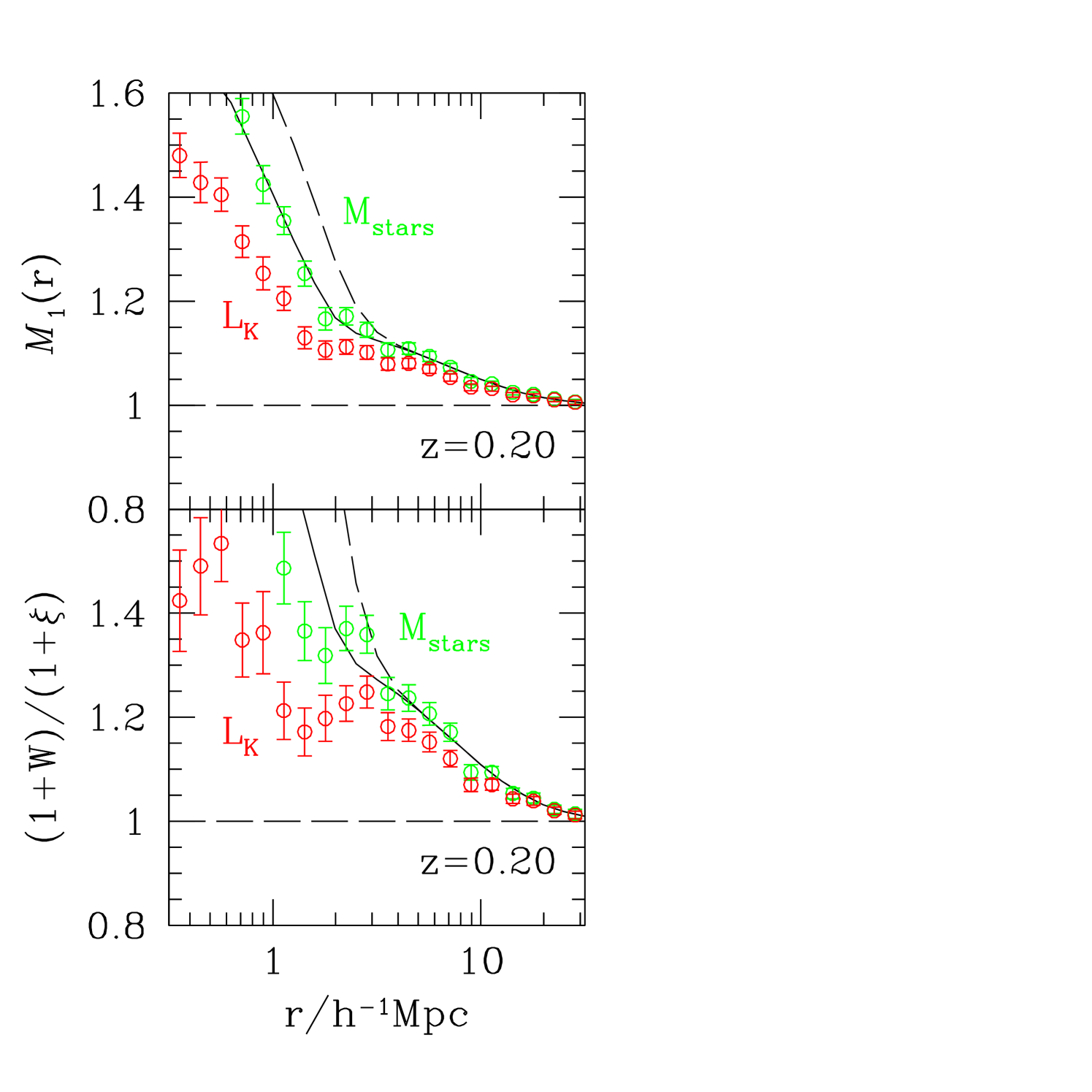
Figure 8: Marked statistics in which $K$-band luminosity and stellar mass were used as marks. Symbols show measurements in the GIF semi-analytic galaxy formation models, and dotted curves show an estimate of the uncertainty on the measurement. Dashed and solid curves show the halo-model calculation for each statistic when $M_{\rm star}$ is the mark (the halo-model calculations for $L_{K}$ are shown in Figure 3.) The solid curves are the result of including the fact that the central galaxy in a halo is different from the others.

The simplest halo model calculations presented here indicate that the lowest order marked statistics ${\cal M}_{1}(r)$ and $W(r)$ encode information about the mean correlation between mark and halo-mass. (Note that this information is provided without ever actually dividing the galaxy distribution up into ‘clusters’.) However, this quantity can be estimated from other methods. For instance, Zehavi et al. (2005) describe a halo-model interpretation of the luminosity dependence of clustering in the SDSS by studying clustering in subsamples defined by galaxy luminosity. Their analysis can be used to infer how the mean luminosity of a galaxy correlates with the mass of its host halo, provided one assumes that the environment plays no additional role than through halo biasing. Therefore, insertion of their luminosity-mass correlations in the halo model description developed here represents a prediction for the shape of the luminosity-marked correlations in the SDSS. If this prediction agrees with the actual measurement of marked statistics in the SDSS, then this will provide strong empirical justification for the assumption that there are no additional environmental effects. This test is the subject of Skibba, Sheth & Connolly (2005).

One may turn this statement around, and ask if the luminosity weighted marked statistics (${\cal M}_{1}$ or $W$) provide any new information than one gets from analysis of the luminosity dependence of clustering. Clearly, marked statistics provide information about environmental effects which the other method does not. However, if there are indeed no additional environmental effects, then our analysis shows that the two methods provide equivalent information vis a vis correlations between marks and halo masses. Even in this case, however, marked statistics are an attractive choice because they are substantially simpler to estimate (random catalogs are unnecessary), and they do not require division of the catalog into small luminosity bins to calibrate the correlation between mark and halo mass, thus allowing a higher signal-to-noise measurement from a larger catalog (rather than from smaller subsamples split by the value of the mark).

Finally, Figure 8 illustrates another way in which our analysis aids in understanding correlations between galaxy observables and environment. The Figure compares ${\cal M}_{1}$ and $(1+W)/(1+\xi)$ when the mark is $K$-band luminosity (lower set of symbols in each panel) and when stellar mass (upper set of symbols) is the mark. The trends traced out by both marks are the same—close pairs are more luminous and have larger stellar masses—although the amplitude is larger when stellar mass is used as the mark. (To better show that these differences are significant, we have attached the error bars to each set of points, rather than using the same format as in the previous Figures.) The differences between the marked statistics suggest that close pairs have larger mass-to-light ratios. What causes this correlation?

Our halo-model calculation when $M_{\rm stars}$ is the mark is shown as the smooth curve; the analogous calculation for $L_{K}$ was shown in Figure 3. In both cases, the halo-model calculation provides an excellent description of the statistics, at least on scales larger than $2h^{-1}$Mpc for the weighted correlation function, and down to even smaller scales for ${\cal M}_{1}$. This agreement shows that, although the mass-to-light ratio is higher in dense regions, this environmental dependence is entirely due to the individual correlations between halo mass and mass-to-light ratio (Figure 5), and between halo mass and environment. It will be interesting to see if other correlations between observables (e.g., the Fundamental Plane) show environmental trends for similar reasons.

Appendix A Toy model

This Appendix illustrates the ideas presented in the main text using a toy model in which relatively transparent analytic results can be derived, and whose ingredients are qualitatively similar to the more exact calculations shown in the main text. Let

$$\rho(r)=\rho_{s}\,{\exp(-r/r_{s})\over(r/r_{s})^{2}}$$ (35)

denote the density run of the mass around a halo centre. The total mass associated with this profile is

$$M=\int{\rm d}r\,4\pi r^{2}\,\rho(r)=4\pi\,r_{s}^{3}\rho_{s}$$ (36)

The normalized Fourier transform of this profile is

$$u(k)={1\over M}\int{\rm d}r\,4\pi r^{2}\,\rho(r)\,{\sin(kr)\over kr}={{\rm arctan}(kr_{s})\over kr_{s}}.$$ (37)

The correlation function is proportional to the Fourier transform of the square of this quantity.

Now suppose that the probability a galaxy lies at distance $r$ from the center is

$$p(r)\,{\rm d}r={4\pi r^{2}\,{\rm d}r\,\rho(r)\over 4\pi\,r_{s}^{3}\rho_{s}}=\exp(-r/r_{s})\,{{\rm d}r\over r_{s}};$$ (38)

i.e., galaxies trace the mass. Further, suppose that objects which are more distant from the centre are more luminous: $L/L_{*}=r/r_{s}$ for some constant $L_{*}$. Then the distribution of luminosities is

$$p(L)\,{\rm d}L=p(r)\,{\rm d}r=\exp(-L/L_{*})\,{{\rm d}L\over L_{*}}.$$ (39)

Thus, the mean luminosity is $L_{*}$. This will be useful shortly. Note that both the density run $\rho(r)$ and the luminosity distribution $p(L)$ have rather realistic shapes, so the results which follow should resemble the real-world at least qualitatively.

In this model, the run of the luminosity-weighted profile is

$${L(r)\over L_{*}}\,\rho(r)=\rho_{s}\,{\exp(-r/r_{s})\over(r/r_{s})},$$ (40)

so the normalized Fourier transform of this profile is

$$w(k)={\int{\rm d}r\,4\pi r^{2}\,L(r)\,\rho(r)\,\sin(kr)/kr\over\int{\rm d}r\,4\pi r^{2}\,L(r)\,\rho(r)}={1\over 1+k^{2}r_{s}^{2}}.$$ (41)

Hence, the luminosity-weighted correlation function is proportional to $(\pi/4)\,\exp(-r/r_{s})/(2\pi^{2})$. Since $w(k)^{2}/u(k)^{2}\leq 1$ for all $k$, this shows that $W(r)\leq\xi(r)$ for all $r$. Hence, in this model with luminosity increasing with distance from halo center, the marked correlation function $(1+W)/(1+\xi)$ decreases with decreasing $r$.

Note that although there is no scatter in luminosities at fixed $r$, there is scatter in $L$ at fixed pair separation (the two members of a pair of fixed separation can come from different distances from the halo center). Thus, in this model, the variance in weights at fixed pair separation is non-trivial.

Now suppose that we randomize the luminosities within each halo. This means that the total distribution of luminosities is still $p(L)=\exp(-L/L_{*})/L_{*}$, but this distribution now represents the probability that a galaxy in the halo has luminosity $L$ whatever its distance from the halo center. In this case, the result of weighting each galaxy by its luminosity does not yield an $r$ dependent weight, so the weighted profile $(L/L_{*})\,\rho(r)=\rho(r)$, since the mean of the weights $L$ is $L_{*}$. Hence, in this case, $w(k)=u(k)$: the weighted and unweighted correlation functions are equal.

The calculation in the previous section assumes that there is no correlation between weight and position within the parent halo. Hence it can describe the marked statistics associated with the case when the luminosities have been randomized. In this case, the small-scale dependence of the marked correlation function is entirely a consequence of the fact that the mean weight may depend on halo mass. If there is some correlation between weight and galaxy position within the halo, then this will manifest as a discrepancy between the model and the actual measured marked correlation.

As a specific example of why such a discrepancy may be interesting, suppose that the first case (weights increase with increasing distance from halo center) corresponds to the luminosity distribution in a blue band, say $L_{B}$, whereas the second case corresponds to the luminosity in a redder band, say $L_{R}$. The color is defined as $c\equiv L_{R}/L_{B}$. For what follows, it is useful to define $c_{*}=L_{R*}/L_{B*}$. Since $L_{B}$ is a deterministic function of $r$, the color distribution at $r$ is due to the distribution in $L_{R}$: $p(c|r)\,{\rm d}c=p(L_{R}=cL_{B}(r))\,L_{B}(r)\,{\rm d}c=\exp[-(c/c_{*})L_{B}(r)/L_{B*}]\,(L_{B}(r)/L_{B_{*}})\,{\rm d}c/c_{*}$ so the mean color at $r$ is $c_{*}\,L_{B*}/L_{B}(r)=c_{*}\,(r_{s}/r)$. This shows that there is a color gradient: the halo is redder in the center than it is outside. It is this color gradient which gives rise to the difference between the two luminosity-weighted correlation functions. This illustrates that marked correlation functions encode information about luminosity- and hence color-gradients.

References

- [1] Abazajian K., et al., 2003, AJ, 126, 2081
- [2] Beisbart C., Kerscher M., 2000, ApJ, 545, 6
- [3] Beisbart C., Kerscher M., Mecke K., 2002, in K. Mecke and D. Stoyan (eds.), Morphology of Condensed Matter. Physics and Geometry of Spatial Complex Systems. Lecture Notes in Physics, Vol. 600, J. Springer, Berlin, p. 358–390.
- [4] Colless M., et al., 2001, AJ, 328, 1039
- [5] Cooray A., Sheth R. K., 2002, Phys. Rep., 372, 1
- [6] Faltenbacher A., Gottlöber S., Kerscher M., Müller V., 2002, A&A, 395, 1
- [7] Gao L., White S. D. M., Jenkins A., Stoehr F., Springel V., 2004, MNRAS, 355, 819
- [8] Gao L., Springel V., White S. D. M., 2005, MNRAS, accepted
- [9] Gottlöber S., Kerscher M., Kravtsov A. V., Faltenbacher A., Klypin A., Müller V., 2002, A&A, 387, 778
- [10] Kauffmann G., Diaferio A., Colberg J., White S. D. M., 1999, MNRAS, 303, 188
- [11] Kravtsov A. V., Berlind A. A., Wechsler R., Klypin A. A., Gottlöber S., Allgood B., Primack J., 2004, ApJ, 609, 35
- [12] Magliochetti M., Porciani C., 2003, MNRAS, 346, 186
- [13] Mo H. J., White S. D. M., 1996, MNRAS, 282, 347
- [14] Mo H. J., Yang X., van den Bosch F. C., Jing Y. P., 2004, MNRAS, 349, 205
- [15] Peebles P. J. E., 1980, The Large-Scale Structure of the Universe. Princeton Univ. Press, Princeton, NJ
- [16] Sheth R. K., Abbas U., Skibba R. A., 2004, in Diaferio A., ed, Proc. IAU Coll. 195, Outskirts of galaxy clusters: intense life in the suburbs, CUP, Cambridge, p. 349
- [17] Sheth R. K., Jain B., 2003, MNRAS, 345, 529
- [18] Sheth R. K., Tormen G., 1999, MNRAS, 308, 119
- [19] Sheth R. K., Tormen G., 2002, MNRAS, 329, 61
- [20] Sheth R. K., Tormen G., 2004, MNRAS, 350, 1385
- [21] Sheth R. K., Connolly A. J., Skibba R., 2005, MNRAS, submitted
- [22] Skibba R., Sheth R. K., Connolly A. J., 2005, MNRAS, in prep.
- [23] Stoyan D., 1984, Math. Nachr., 116, 197
- [24] Stoyan D., Stoyan H., 1994, Fractals, Random Shapes, and Point Fields. Wiley & Sons, Chichester
- [25] York D., et al., 2000, AJ, 120, 1579
- [26] Zehavi I., et al., 2005, ApJ, in press, astro-ph/0408569
- [27] Zentner A. R., Berlind A. A., Bullock J. S., Kravtsov A. V., Wechsler R. H., 2005, ApJ, 624, 505
- [28] Zheng Z., et al., 2005, ApJ, submitted, astro-ph/0408564