Modelling Galaxies with a 3d Multi-Phase ISM

We present a new particle code for modelling the evolution of galaxies. The code is based on a multi-phase description for the interstellar medium (ISM). We included star formation (SF), stellar feedback by massive stars and planetary nebulae, phase transitions and interactions between gas clouds and ambient diffuse gas, namely condensation, evaporation, drag and energy dissipation. The latter is realised by radiative cooling and inelastic cloud-cloud collisions. We present new schemes for SF and stellar feedback. They include a consistent calculation of the star formation efficiency (SFE) based on ISM properties as well as a detailed redistribution of the feedback energy into the different ISM phases.

As a first test example we show a model of the evolution of a present day Milky-Way-type galaxy. Though the model exhibits a quasi-stationary behaviour in global properties like mass fractions or surface densities, the evolution of the ISM is locally strongly variable depending on the local SF and stellar feedback. We start only with two distinct phases, but a three-phase ISM is formed soon consisting of cold molecular clouds, a warm gas disk and a hot gaseous halo. Hot gas is also found in bubbles in the disk accompanied by type II supernovae explosions. The volume filling factor of the hot gas in the disk is $\sim 35\%$. The mass spectrum of the clouds follows a power-law with an index of $\alpha\approx-2$. The star formation rate (SFR) is $\sim 1.6\,{\rm M}_{\hbox{$\odot$}}\,{\rm yr}^{-1}$ on average decreasing slowly with time due to gas consumption. In order to maintain a constant SFR gas replenishment, e.g. by infall, of the order $1\,{\rm M}_{\hbox{$\odot$}}\,{\rm yr}^{-1}$ is required. Our model is in fair agreement with Kennicutt’s (1998) SF law including the cut-off at $\sim 10\,{\rm M}_{\hbox{$\odot$}}\,{\rm pc}^{-2}$. Models with a constant SFE, i.e. no feedback on the SF, fail to reproduce Kennicutt’s law.

We have performed a parameter study varying the particle resolution, feedback energy, cloud radius, SF time scale and metallicity. In most these cases the evolution of the model galaxy was not significantly different to our reference model. Increasing the feedback energy by a factor of $4-5$ lowers the SF rate by $\sim 0.5\,{\rm M}_{\hbox{$\odot$}}\,{\rm yr}^{-1}$ and decreasing the metallicity by a factor of $\sim 100$ increases the mass fraction of the hot gas from about 10% to 30%.

1 Introduction

The treatment of the instellar medium (ISM) is a crucial part in modelling galaxies due to the importance of dissipation, star formation (SF) and feedback. Single-phase TREE-SPH models suffer from over-cooling (Pearce et al. 1999; Thacker et al. 2000) because the multi-phase structure of the ISM is not resolved. As a result baryonic matter loses angular momentum to the dark matter (DM) halos and the disks formed in these simulations are too concentrated. Also, SF is overly efficient. On the other hand, a multi-phase ISM is a pre-requisite for the classical grid-based chemo-dynamical (CD) models (Burkert et al. 1992; Theis et al. 1992; Samland et al. 1997; Samland & Gerhard 2003) but they lack the geometrical flexibility of a (3d-)particle code.

An approach to include a multi-phase treatment of the ISM in a particle code has been presented by Semelin & Combes (2002), who combined Smoothed Particles Hydrodynamics (SPH) with a sticky particle method (Carlberg 1984; Combes & Gerin 1985; Noguchi 1988; Palouš et al. 1993; Theis & Hensler 1993). In the multi-phase ISM code of Semelin & Combes (2002) sticky particles are used to describe a cold, dense cloudy medium while the diffuse ISM is modelled by SPH. Stars form from cold gas and feedback processes include heating of cold gas by supernovae and stellar mass loss (including metal enrichment). Cooling leads to a phase transition from warm to cold gas. The main advantage of this approach is the dynamical treatment of the cloud component: clouds are assumed to move on ballistic orbits dissipating kinetic energy in collisions.

The main purpose of this paper is to present a new extended TREE-SPH code with a multi-phase description of the ISM adopted from CD models. Similar to Semelin & Combes (2002), this is achieved by a combination of a sticky particle scheme and SPH. However, we use a different sticky particle scheme based on an individual treatment of single clouds. Advantages of this scheme are the build-up of a cloud mass spectrum, the individual handling of cloud collisions and the localised treatment of phase transitions between clouds and the ambient diffuse gas. Furthermore, we apply a refined SF recipe suggested by Elmegreen & Efremov (1997, hereafter EE97). This scheme considers star formation within individual clouds including local feedback processes. As a result the star formation efficiency is locally variable depending on the cloud mass and the ambient ISM pressure.

A detailed description of the model including all the processes is given in Sect. 2. Details on the numerical treatment can be found in Sect. 3. The code is applied to an isolated Milky-Way-type galaxy (Sect. 4). The results (including a short parameter study) are discussed in Sect. 5. Conclusions and future applications of this code are presented in Sect. 6.

2 The Model

Figure 1: The network of processes connecting the different gaseous and stellar components. Clouds are the sites of SF. Stars return mass and inject energy to the multi-phase ISM. The two gas phases exchange mass and momentum by means of condensation or evaporation and drag. Dissipation of energy is due to radiative cooling and cloud-cloud collisions.

We use particles to describe all galactic components. Each particle is assigned a special type representing either stars, clouds, (diffuse) gas or DM. The different components are connected by a network of processes including SF, stellar feedback, cooling, cloud-cloud collisions, condensation, evaporation and drag as shown schematically in Fig. 1.

2.1 Stars

Each star particle represents a cluster of stars formed at the same time. The initial stellar mass distribution is given by the multi-power law IMF of Kroupa et al. (1993) with the lower and upper mass limits of $0.1\,{\rm M}_{\hbox{$\odot$}}$ to $100\,{\rm M}_{\hbox{$\odot$}}$ respectively.

The stellar life times (depending on stellar mass and metallicity) are approximated according to Raiteri et al. (1996) to give reasonable fits to the Padova evolutionary tracks (Alongi et al. 1993; Bressan et al. 1993; Bertelli et al. 1994) in the mass range from $0.6\,{\rm M}_{\hbox{$\odot$}}$ to $120\,{\rm M}_{\hbox{$\odot$}}$ and for metallicities ${\rm Z}=7\cdot 10^{-5}-0.03$.

We assume that stars with masses above $8\,{\rm M}_{\hbox{$\odot$}}$ end their life as type II supernovae (SNII) and stars from $1-8\,{\rm M}_{\hbox{$\odot$}}$ end as planetary nebulae (PNe). The mass fractions of these stars are $9\%$ and $34\%$ respectively. The life times of the high mass stars range from $3\,{\rm Myr}$ to $39\,{\rm Myr}$. The stellar feedback is described below.

2.2 Clouds

The cloud particles describe a cold, clumpy phase of the ISM, i.e. the molecular clouds, which are also the sites of SF. The radius $r_{\rm cld}$ of an individual cloud is given by the following relation based on observations (Rivolo & Solomon 1988):

$$r_{\rm cld}=A_{\rm cld}\cdot\sqrt{m_{\rm cld}\over 10^{6}\,{\rm M}_{\hbox{$\odot$}}}\,{\rm pc},$$ (1)

where the constant $A_{\rm cld}$ is set to $50$.

The giant molecular clouds represented by cloud particles consist of gas at different densities and temperatures. Since we do not resolve this structure we do not define a temperature or pressure for individual clouds. However, we assume that the clouds are influenced by the pressure of the surrounding ISM (see Sect. 2.6). Radiative cooling within clouds is not taken into account. However, we allow for dissipation of kinetic energy in cloud-cloud collisions using the dissipation scheme of Theis & Hensler (1993). Two clouds undergo a complete inelastic collision if they physically collide within the next time step. Additionally, their orbital angular momentum must be less than the break-up spin of the final cloud and the cloud mass must not exceed a critical mass limit (here: $M_{\rm coll,lim}=1\cdot 10^{7}\,{\rm M}_{\hbox{$\odot$}}$). In case of a sticky collision the two cloud particles are replaced by one particle keeping the center-of-mass data of the former two clouds.

2.3 Diffuse gas

In an first approximation the diffuse gas can be described as continuous self-gravitating fluid. We model this component using an SPH approach. The gas is assumed to obey the ideal equation of state with adiabatic index $\gamma=5/3$:

$$P_{\rm gas}=(\gamma-1)\rho_{\rm gas}u,$$ (2)

where $P_{\rm gas}$ is the pressure, $\rho$ the density and $u$ the energy per unit mass of the gas. The thermal energy evolution is governed by cooling and heating processes. For the latter we only take the most dominant source, the SNII, into account. Dissipation is performed by the metal-dependent cooling function from Böhringer & Hensler (1989).

The diffuse gas can have temperatures from a few $10^{3}\,{\rm K}$ up to several $10^{6}\,{\rm K}$. In the following we will also distinguish between warm and hot gas meaning gas at temperatures below or above $10^{4}\,{\rm K}$ respectively.

2.4 Dark Matter

In our code DM can be modelled either with particles (live halo) or as a static potential. In this work we focus on the late evolution of an isolated galaxy where a static DM potential is a reasonable approximation. We use the potential from Kuijken & Dubinski (1995) which is a flattened, isothermal potential with a core and a finite extent.

2.5 Interactions between the ISM phases

The ISM is treated as two dynamically independent gas phases. This approach has been successfully applied in chemo-dynamical models (Theis et al. 1992; Samland et al. 1997). The two gas phases are linked by two processes: condensation/evaporation (C/E) and a drag force. Following Cowie et al. (1981) the mass exchange rate by condensation and evaporation for an individual cloud particle is calculated from

$$\begin{array}[]{ll}\dot{m}_{\rm cld}&=\left({\displaystyle\frac{T_{\rm gas}}{\,{\rm K}}}\right)^{2.5}{\displaystyle\frac{r_{\rm cld}}{\,{\rm pc}}}\\ &\cdot\left\{\begin{array}[]{llllll}-2.75\cdot 10^{4}\sigma_{0}^{-5/8}&{\rm if}&&&\sigma_{0}&>1\\ -2.75\cdot 10^{4}&{\rm if}&0.03&<&\sigma_{0}&\leq 1\\ 8.25\cdot 10^{2}\sigma_{0}^{-1}&{\rm if}&&&\sigma_{0}&\leq 0.03\end{array}\right.\,{\rm g}\,{\rm s}^{-1},\end{array}$$ (3)

where the parameter $\sigma_{0}$ is defined as

$$\sigma_{0}=\left({T_{\rm gas}\over 1.54\cdot 10^{7}\,{\rm K}}\right)^{2}\left({r_{\rm cld}\over\,{\rm pc}}\right)^{-1}\left({n_{\rm gas}\over\,{\rm cm}^{-3}}\right)^{-1}.$$ (4)

$T_{\rm gas}$ and $n_{\rm gas}$ are the local temperature and number density of the diffuse gas. The clouds are subject to a drag force ${\bf F}_{\rm D}$ due to ram pressure which is given by (Shu et al. 1972)

$${\bf F}_{\rm D}=-C_{\rm D}\,\pi r_{\rm cld}^{2}\,\rho_{\rm gas}\,v_{\rm rel}\,{\bf v}_{\rm rel},$$ (5)

where $\rho_{\rm gas}$ is the local gas density and $v_{\rm rel}$ is the velocity of the cloud relative to the gas. The constant $C_{\rm D}$ is not well determined and it can be in the range $0.1-1$. We used $C_{\rm D}=0.1$.

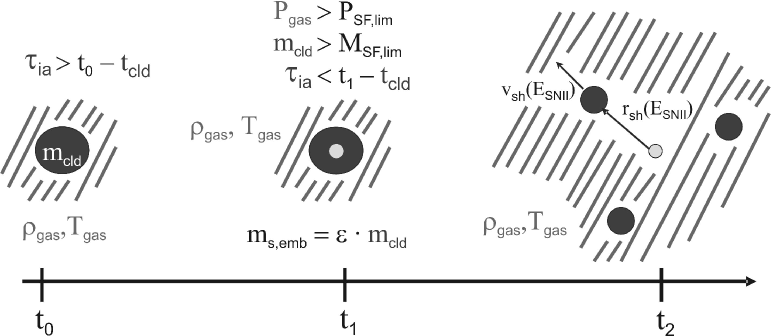
Figure 2: The diagram shows the SF scheme: ($t_{0}$) the cloud is inactive (no SF); ($t_{1}$) an embedded star cluster has been formed with a local SF efficiency; ($t_{2}$) the cloud is fragmented by SNII energy input.

2.6 Star Formation

The treatment of SF is usually based on the Schmidt Law (Schmidt 1959)

$${\rm SFR/area}=c_{n}\cdot\Sigma_{g}^{n},$$ (6)

with the gas surface density $\Sigma_{g}$ and $n\approx 1.5$. The parameter $c_{n}$ combines a SF time scale and a SFE. A reasonable estimate for the time scale is given by the dynamical time. The SFE on the other hand cannot be determined from current theories of SF and therefore remains a free parameter. A constant SFE also cannot account for local feedback processes, by this prohibiting any self-regulation of the SF. However, Köppen et al. (1995) have demonstrated the importance of negative stellar feedback which leads to a Schmidt-type strongly self-regulated SF.

Though the standard approach for SF works well for isolated galaxies, it has difficulties in reproducing observations of interacting galaxies (Mihos et al. 1992, 1993).Barnes (2004) suggested a second shock-induced SF mode. However, this means another free parameter in the SF recipe.

Different to such an approach, we applied a single SF law, but with a temporally and spatially variable SFE suggested by EE97. They assign each molecular cloud an individual star formation efficiency which is controlled by the ISM properties (mass of the molecular cloud, pressure of ambient diffuse gas) and the stellar feedback. According to EE97 the star formation is most efficient for massive clouds embedded in a high pressure ambient medium. A pre-requisite of using the EE97 SFE scheme is a multi-phase treatment of the ISM as proposed in this paper.

The main concept of our SF implementation is that stars form in clouds and clouds are destroyed by stellar feedback and, thus, self-regulating the SF (Fig. 2). Each cloud is assumed to form stars only after a time of inactivity $\tau_{\rm ia}$ (${\rm t}_{0}$ in Fig. 2), because not all gas in clouds is dense or unstable enough for immediate SF. Once the SF process has started, an embedded star cluster is formed (${\rm t}_{1}$) instantaneously .

Following EE97 we use a variable SF efficiency $\epsilon$ depending on local properties of the ISM. A typical SFE (cloud mass of $10^{4}-10^{6}\,{\rm M}_{\hbox{$\odot$}}$ and pressure typical for solar vicinity) is between 5% and 10% (see Fig. 4 in EE97). For details of the implementation see App. A.

The only free parameter in our SF recipe is $\tau_{\rm ia}$. It can be interpreted as a global SF time scale: assuming a SFE of $\epsilon\sim 0.1$, a total mass $M_{\rm cld}$ in clouds of a few $10^{9}\,{\rm M}_{\hbox{$\odot$}}$ and $\tau_{\rm ia}$ of a few $100\,{\rm Myr}$ , we get a global ${\rm SFR}\sim\epsilon M_{\rm cld}\tau_{\rm ia}^{-1}$ of $\sim 1\,{\rm M}_{\hbox{$\odot$}}\,{\rm yr}^{-1}$.

2.7 Stellar Feedback

Once the SFE has been determined the energy released by SNII in each time step can be computed from the chosen IMF and stellar life times (Sect. 2.1). We assume $\epsilon_{\rm SN}=2\cdot 10^{50}\,{\rm erg}$ for the energy released per SNII event.

This energy injection disrupts the cloud into smaller fragments (${\rm t}_{2}$ in Fig. 2) leaving a new stellar particle. The time for disruption $t_{\rm dis}$ ($={\rm t}_{2}-{\rm t}_{1}$) is determined from the energy input: in our model the energy input of the SNII drives an expanding shell into the cloud. The cloud mass is accumulated in this shell. The expansion of the SN shell can be calculated from a self-similar solution (Brown et al. 1995; Theis et al. 1998). Assuming a spherical cloud with a $1/r$-density profile in agreement with the mass-radius relation (Eq. 1) we get

$$r_{\rm sh}(t)=0.918\left({\dot{E}\over\rho_{1}}\right)^{0.25}\cdot t^{0.75},$$ (7)

$$v_{\rm sh}(t)=0.689\left({\dot{E}\over\rho_{1}}\right)^{0.25}\cdot t^{-0.25},$$ (8)

where $\dot{E}$ is the energy injection rate and $\rho_{1}=m_{\rm cld}/r_{\rm cld}^{2}$.

It is assumed that the cloud is disrupted when the shell radius reaches the cloud radius. The fragments are then placed symmetrically on the shell with velocities corresponding to the expansion velocity at $t_{\rm dis}$. The energy not consumed by cloud disruption, i.e. the energy of SNII exploding after $t_{\rm dis}$, is returned as thermal feedback to the hot gas phase. Depending on cloud mass and SF efficiency the fragmentation uses about 0.1–5% of the total SNII energy of which $\sim 20\%$ end up as kinetic energy of the fragments.

The mass returned by SNII is also added to the surrounding gas. It is determined from the IMF and stellar life times assuming that the mass ejected per SNII event $M_{\rm SNII,ej}$ is given by (Raiteri et al. 1996)

$$M_{\rm SNII,ej}(m)=0.77m^{1.06}\,{\rm M}_{\hbox{$\odot$}},$$ (9)

where $m$ is the mass of a star.

Additionally to the SNII feedback, we also allow for feedback by PNe. After each time step, the mass $M_{\rm PN}$ returned to the ISM by PNe is calculated by assuming that the PN mass ejected by a star of mass $m$ is given by (Weidemann 2000)

$$M_{\rm PN,ej}(m)=0.91m-0.45\,{\rm M}_{\hbox{$\odot$}}.$$ (10)

Gradual metal enrichment due to stellar mass release and type I SNe are not included so far. This is justified for the kind of models presented here (s. Sect. 4.1) as metal enrichment has little effect as we show later (s. Sect. 5.3).

3 Numerical Treatment

3.1 Stellar Dynamics

In our code the gravitational force on a particle can be calculated as a combination of the self-gravity of the N-body system and an external force. External forces – if applied – usually mimic a static dark matter halo. Self-gravity is calculated using a tree scheme. We have included two different tree schemes: the widely used scheme of Barnes & Hut (1986) and a new tree algorithm proposed by Dehnen (2002). An advantage of the Dehnen-TREE is that it is momentum-conserving by construction. Additionally, an error control is included and the CPU scaling is basically linear with the number of particles. In our implementation the Dehnen-TREE is more than an order of magnitude faster than the Barnes&Hut-TREE. Hence, we applied here mainly the Dehnen-TREE. For easy comparison with other N-body solvers we realised gravitational softening by a Plummer potential with a softening length ${\epsilon}_{\rm s}=0.1\,{\rm kpc}$.

3.2 Gas Dynamics

We use the SPH formalism to compute the hydrodynamics of the diffuse gas and a sticky particle scheme for the clouds. Details of our SPH implementation are described in App. B.

The dynamics of the clouds are described by the sticky particle scheme of Theis & Hensler (1993). According to them clouds move on ballistic orbits unless they undergo inelastic collisions. The treatment of cloud-cloud collisions is described in Sect. 2.2.

3.3 Time Integration

The time integration of the system is done with a leap-frog scheme. Individual time steps are used for each particle. The time step for an SPH particle $p$ is chosen to satisfy a modified form of the Courant condition (for details see App. B). The time step of all other particles is based on dynamical criteria calculated by

$$\Delta t_{p}\leq\eta_{\rm ts}\cdot\min\left({{\epsilon}_{\rm s}\over v_{p}},\sqrt{{\epsilon}_{\rm s}\over a_{p}}\right),$$ (11)

where $a_{p}$ is the acceleration and ${\epsilon}_{\rm s}$ the softening length of particle $p$. The constant $\eta_{\rm ts}$ is of the order of unity (we set it to 0.4).

The largest individual time step $\Delta t_{p}$ also defines the system time step $\Delta t_{\rm sys}$ which is further limited not to exceed $\sim 1\,{\rm Myr}$. Individual particle time steps are chosen to be a power-of-two subdivision of $\Delta t_{\rm sys}$ (Aarseth 1985).

3.4 Mass exchange and new particles

Several processes included in our model lead to an exchange of mass between particles or the creation or removal of particles. These processes are introduced in a matter- and momentum-conserving manner.

The mass exchange by condensation and evaporation is calculated after each system time step $\Delta t_{\rm sys}$. The transferred mass $\dot{m}_{\rm cld}\Delta t_{\rm sys}$ is added to the cloud. The same mass is subtracted from the surrounding SPH particles taking into the account the weighting from the kernel function. Additionally, the velocity of particles gaining mass (i.e. clouds in case of condensation and SPH particles for evaporation) is changed in order to conserve momentum. The mass exchange from stars to SPH particles (SNII) and clouds (PNe) is done in a similar way.

Whenever a SF process occurs, the star forming cloud is removed from the simulation. Instead a new star particle of the mass $\epsilon m_{\rm cld}$ is added at the same position with the same velocity. Furthermore, the clouds formed in expanding shells are created by adding four new cloud particles carrying the remaining mass. Their positions and velocities are chosen according to Eq. (7) and (8) thus conserving mass and momentum.

3.5 Mass limits for particles

Our model allows particles to be created, merged and changed in mass. A few constraints are used for the sake of numerical accuracy and particle numbers.

In order to prevent the formation of too many low mass star particles a lower mass limit $M_{\rm SF,lim}=2.5\cdot 10^{4}\,{\rm M}_{\hbox{$\odot$}}$ and a lower pressure limit $P_{\rm SF,lim}=0.1P_{\hbox{$\odot$}}$ for SF are introduced.

The maximum mass for clouds is given by $M_{\rm coll,lim}$ (Sect. 2.2) but a lower mass limit for clouds $M_{\rm cld,lim}$ is also set to

$$M_{\rm cld,lim}=0.1M_{\rm SF,lim}.$$ (12)

If the mass of a cloud becomes smaller than $M_{\rm cld,lim}$ the particle is removed from the system and the mass is distributed evenly among neighbouring cloud particles within $300\,{\rm pc}$.

SPH particles can change their mass due to condensation and evaporation. In order to avoid SPH particles getting too massive an upper mass limit is introduced. Whenever an SPH particle reaches this limit it is split into four new particles. The new equal mass particles have the same center of mass, velocity, angular momentum and specific energy as the particle they replace. A lower mass limit is also used where the mass of an SPH particle is distributed to the neighbouring particles. The upper and lower mass limits are set to $4\,m_{\rm SPH}$ and $0.1\,m_{\rm SPH}$ respectively, where $m_{\rm SPH}$ is the SPH particle mass at the beginning of the simulation.

3.6 Tests

We have tested our code thoroughly. Energy and angular momentum conservation is better than 1% for a pure $N$-body simulation following the evolution of a disk galaxy over many rotational periods. We tested our SPH implementation with the standard Evrard-test (Evrard 1988) and find that energy conservation is within 3%. In a full model, angular momentum is conserved within 3%.

4 Disk galaxy model

4.1 Initial Conditions

Table 1: Properties of the initial disk galaxy model

component	mass1	radius2	No. of particles
disk	0.34	18.0	20000
stars	0.27		16000
clouds	0.07		4000
bulge	0.17	4.0	10000
DM halo	1.94	87.9	-
hot gas	0.01	25.	5000
total	2.47		35000
1 in units of $10^{11}\,{\rm M}_{\odot}$, 2 in kpc

A galaxy similar to the present-day Milky Way was set up using the galaxy building package described by Kuijken & Dubinski (1995, hereafter KD95). The models of KD95 consist of three components: the baryonic disk and bulge, and a DM halo. A distribution function for each component yields a unique density for a given potential. By solving the Boltzmann equation for the combined system the galaxy can be set up in a self-consistent way. By construction these models are in virial equilibrium. KD95 have also demonstrated that their models are stable over many rotation periods.

We chose model A of KD95 as a reference model (Tab. 1). The scale length of the disk is $R_{\rm d}=4\,{\rm kpc}$. The total mass of the galaxy is $2.47\cdot 10^{11}\,{\rm M}_{\hbox{$\odot$}}$. The mass and radius of the disk are set to $0.34\cdot 10^{11}\,{\rm M}_{\hbox{$\odot$}}$ and $18.0\,{\rm kpc}$. The corresponding parameters for the bulge are $0.17\cdot 10^{11}\,{\rm M}_{\hbox{$\odot$}}$ and $4.0\,{\rm kpc}$ and for the DM halo $1.94\cdot 10^{11}\,{\rm M}_{\hbox{$\odot$}}$ and $87.9\,{\rm kpc}$, respectively. The particle numbers for disk and bulge, $N_{\rm d}=20\,000$ and $N_{\rm b}=10\,000$, are chosen to have particles of nearly equal mass. The DM halo is added as a static potential. The disk is initially in rotational equilibrium with a small fraction of disordered motion superimposed. This results in a Toomre parameter $Q\equiv\kappa\sigma_{R}/(3.36G\Sigma)$ exceeding 1.9 all over the disk. Thus, according to Polyachenko et al. (1997) the disk is stable against all axisymmetric and non-axisymmetric perturbations.

A cloudy gas phase is added by treating every fifth particle from the stellar disk as a cloud. The total mass in clouds is $M_{\rm cld}\approx 6.9\cdot 10^{9}\,{\rm M}_{\odot}$ and each cloud is randomly assigned a time of inactivity $\tau_{\rm ia}$ between $0$ and $200\,{\rm Myr}$. Initially, all clouds have the same mass ($\sim 1.7\cdot 10^{6}\,{\rm M}_{\hbox{$\odot$}}$) but a mass spectrum is built-up within the first Gyr of evolution.

Finally, a diffuse gas component with a total mass of ${\rm M}_{\rm gas}=1\cdot 10^{9}\,{\rm M}_{\odot}$ is added. This is more difficult because no simple equilibrium state exists for this gas phase: it is not only affected by the gravitational potential but also by cooling and heating processes. The latter varies locally and temporally so that the diffuse gas can only reach a dynamical equilibrium as is also revealed in high-resolution simulations of the ISM (de Avillez & Breitschwerdt 2004). Testing different initial setups, starting far from equilibrium (for the diffuse component only), turned out to be most efficient. Then, the diffuse gas phase relaxes on a few dynamical timescales to a quasi-equilibrium state. In detail, we started with a slowly rotating homogeneous gaseous halo with a radius of $25\,{\rm kpc}$ and a temperature of $5.4\cdot 10^{4}\,{\rm K}$ which relaxed to a quasi-equilibrium within a few 100 Myr.

Since we do not follow the chemical evolution of the galaxy, we apply solar abundances where a metallicity is needed. In order to treat the feedback of ’old’ star particles each star particle is assigned an age. For the bulge stars the age is $10\,{\rm Gyr}$ and for disk stars $0-10\,{\rm Gyr}$.

4.2 Evolution of the Reference Model

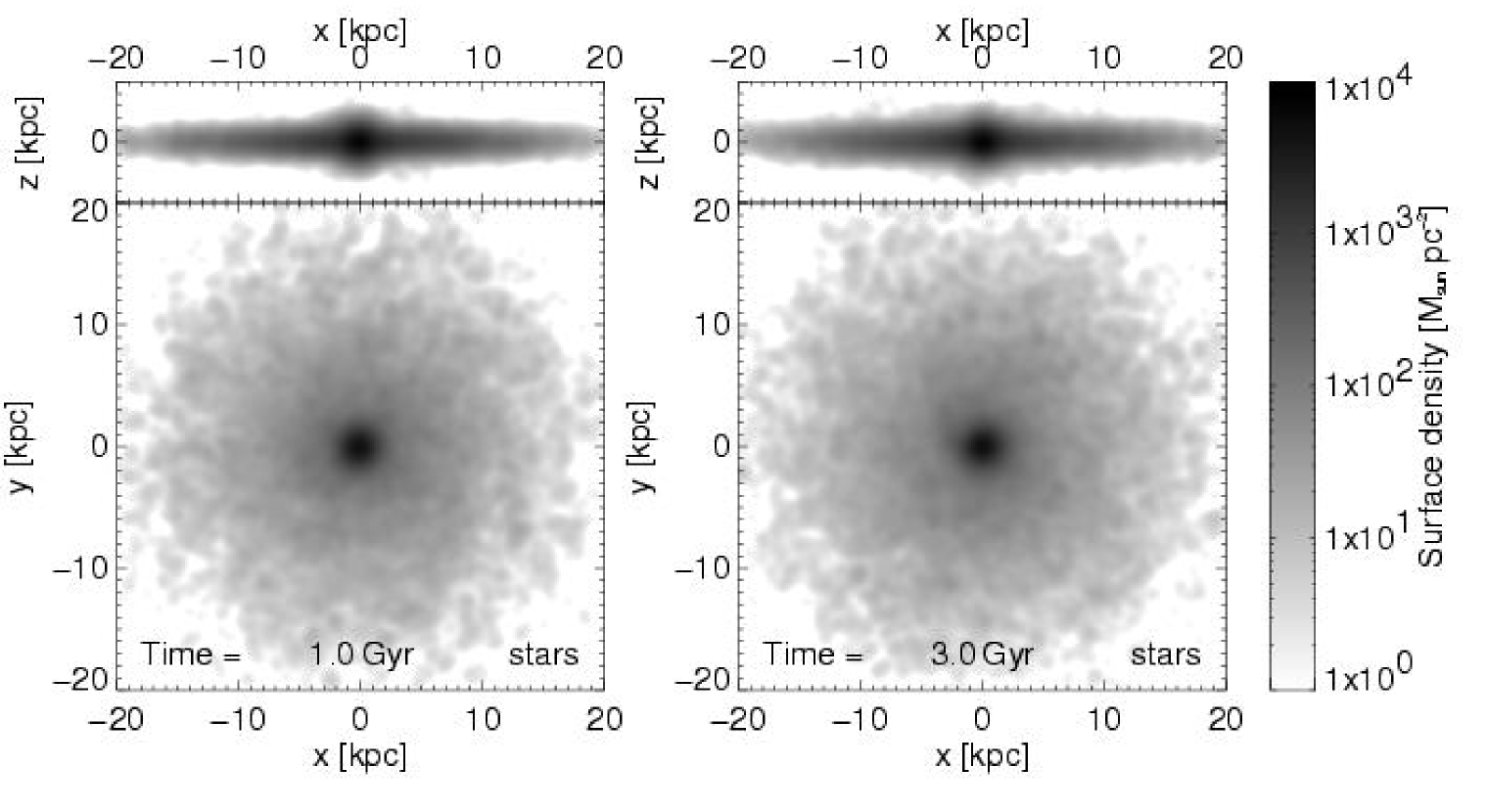
Figure 3: The evolution of stellar surface density (at $1\,{\rm Gyr}$ and $3\,{\rm Gyr}$). The stellar disk becomes slightly thicker with time but is otherwise stable with weak transient spiral patterns. The surface density plots (Fig. 3 and 4) were computed using the NEMO Stellar Dynamics Toolbox (Teuben 1995). The particles were binned in a grid with a cell size of $40\,{\rm pc}$. The resulting map was then smoothed with a Gaussian kernel with ${\rm FWHM}=1\,{\rm kpc}$.

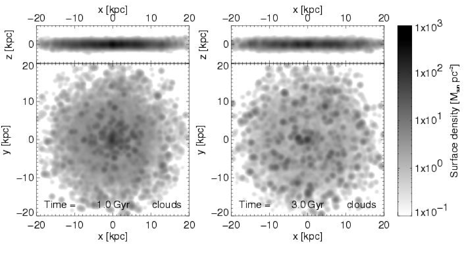
Figure 4: The evolution of cloud surface density (at $1\,{\rm Gyr}$ and $3\,{\rm Gyr}$). The cloud disk is stable but the overall surface density is slowly decreasing. For details on how the surface density was computed see Fig. 3

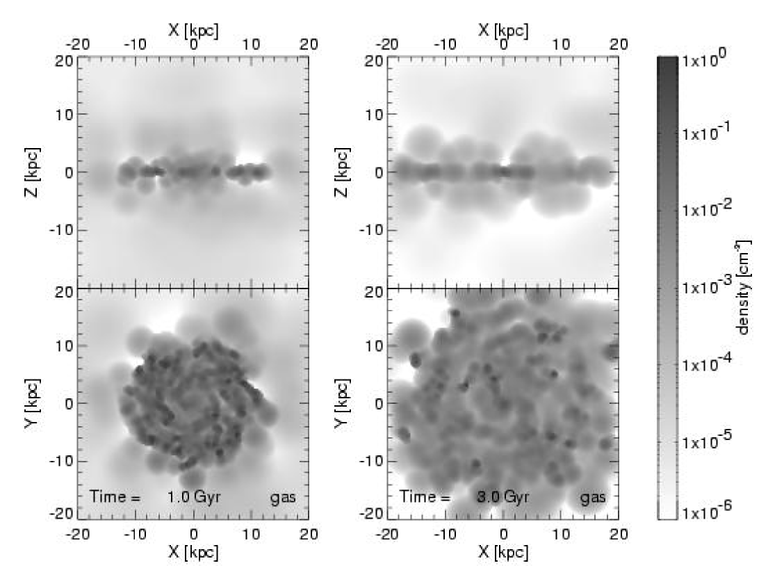
Figure 5: The of evolution of gas density (at $1\,{\rm Gyr}$ and $3\,{\rm Gyr}$). In each panel the xy- (bottom), xz-projection (top) and density scale are shown. Starting from a homogenous distribution the diffuse gas collapses and forms a thin gas disk within $1\,{\rm Gyr}$. While the mass of the gaseous disk is nearly constant its radius is growing slowly. Densities in the disk are of the order of $1\,{\rm cm}^{-3}$. The halo has densities from $10^{-4}\,{\rm cm}^{-3}$ to $10^{-6}\,{\rm cm}^{-3}$. Densities were computed on a $100$x$100$-grid using the SPH formalism.

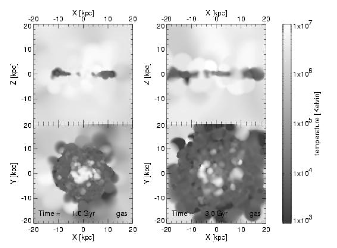
Figure 6: The evolution of gas temperature (at $1\,{\rm Gyr}$ and $3\,{\rm Gyr}$). In each panel the xy- (bottom), xz-projection (top) and temperature scale are shown. After the initial collapse the diffuse gas forms a disk at about $10^{4}\,{\rm K}$. The central part of the disk as well as small bubbles in the outer parts are heated by SNII to $10^{6}\,{\rm K}$. The halo gas it at $10^{6}-10^{7}\,{\rm K}$.

Figure 7: The evolution of the SFR with time (full line). The SFR decreases with time due to consumption of cloud mass. The average SFR (dashed line) is $\approx 1.6\,{\rm M}_{\hbox{$\odot$}}\,{\rm yr}^{-1}$. The dotted line is the result of a simple analytic model accounting for the depletion of the cloudy medium by SF.

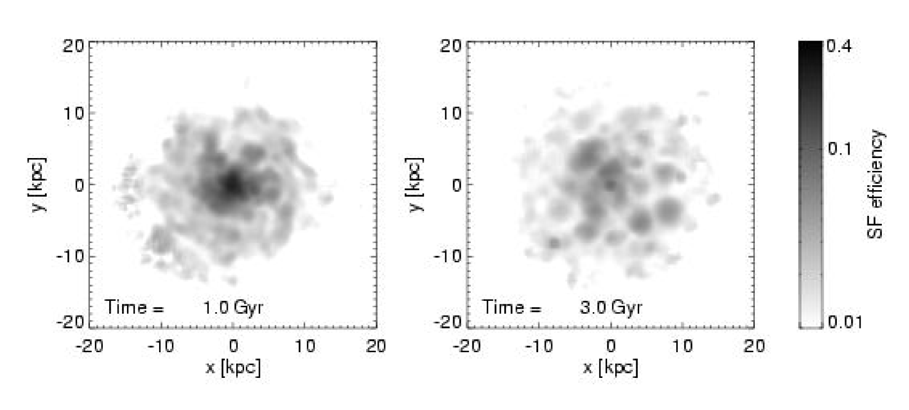
Figure 8: The evolution of SF efficiency . SFE is up to $0.4$ in the center of the galaxy. The average over the whole disk is about $0.06$.

Figure 9: The open diamonds show the SFR per $\,{\rm pc}^{2}$ averaged over $100\,{\rm Myr}$ as a function of cloud surface density. The full line is a recent determination of the Schmidt Law by Kennicutt (1998) with a slope of $-1.4$. The vertical dashed line indicates a cut-off density for SF in disk galaxies also found by Kennicutt (1998).

Figure 10: The cloud mass spectrum. The different lines correspond to the mass spectrum after $1\,{\rm Gyr}$ (dotted), $2\,{\rm Gyr}$ (dashed) and $3\,{\rm Gyr}$ (full) of evolution. The fitted power-law mass function is with $\alpha\approx-2.0$ comparable to the observed mass spectrum.

Starting from these initial conditions the galaxy model is evolved for $3\,{\rm Gyr}$ with all processes switched on. After an initial phase ($500\,{\rm Myr}$) dominated by the collapse of the gaseous halo the galaxy reaches a quasi-equilibrium defined by the interplay of the gravitational potential, radiative cooling, heating by SNII and condensation and evaporation. When the equilibrium is reached the diffuse gas phase has formed a warm disk and a hot halo component. Their mass ratio of about $7$ remains nearly constant for the rest of the simulation. The equilibrium state reached is almost independent of intial setup of the gas halo, i.e. the following evolution is not influenced by our choice.

Snapshots of the evolution of the Milky Way model can be seen in Fig. 3 to 6. The stellar surface density plots in Fig. 3 demonstrate the stability of the disk during the $3\,{\rm Gyr}$ evolution. Profiles of the surface density show that the radial mass distribution does not change except for the central $2\,{\rm kpc}$ where the surface density is increased by up to a factor of $5$ caused by the dissipation-induced infall of clouds which later form stars. Face-on views show weak transient spiral patterns, e.g. at $t=2\,{\rm Gyr}$. Edge-on views reveal a thickening of the disk. Throughout the disk the 95%-mass height $z_{\rm 95,str}$ increases by 47% from $0.75\,{\rm kpc}$ to about $1.1\,{\rm kpc}$. Only in the central $2\,{\rm kpc}$ can no thickening be seen.

The evolution of the cloudy phase (Fig. 4) is influenced by dissipation and SF. The depletion of the cloudy medium by SF decreases its mean surface density. Due to inelastic cloud-cloud collisions the clouds also show a less smooth distribution. As a consequence a mass flow towards the center increases its central surface density. The radial profiles reveal that the surface density has decreased mostly around $5\,{\rm kpc}$ while it it almost unchanged beyond $10\,{\rm kpc}$. The cloud disk shows a thickening only outside of $11\,{\rm kpc}$ where the increase of $z_{\rm 95,cld}$ is very similar to that of the stellar disk. Inside that radius no thickening can be seen. In fact, due to dissipation $z_{\rm 95,cld}$ is even reduced inside $5\,{\rm kpc}$ by a factor of 2–3.

The diffuse gas (Fig. 5) starts from a homogeneous distribution which collapses in less than $300\,{\rm Myr}$ to form a disk. Initially, the gaseous disk is only a few kpc in diameter but it is slowly growing in size. After $1\,{\rm Gyr}$ it has reached a diameter of $20\,{\rm kpc}$. At $2\,{\rm Gyr}$ the diameter is $\sim 30\,{\rm kpc}$ which is comparable to that of the stellar disk. At the same time the mass of the gaseous disk is nearly constant. It has particle densities of $0.1-1\,{\rm cm}^{-3}$ and temperatures (Fig. 6) of less than $10^{4}\,{\rm K}$. Towards the center the gas reaches higher temperatures of up to several $10^{6}\,{\rm K}$. Some diffuse gas remains in the halo at densities of $\sim 10^{-4}\,{\rm cm}^{-3}$ and less while its temperature is in the range of $10^{6}-10^{7}\,{\rm K}$. During the initial collapse the diffuse gas gains a significant amount of angular momentum transferred from the clouds by the drag force. For this reason the gaseous disk rotates with a rotation velocity of $\sim 200\,{\rm km}\,{\rm s}^{-1}$. Transient spiral patterns are also observed in the gas disk. Stellar feedback induces the emergence of bubbles of hot gas. These bubbles have diameters of up to $1\,{\rm kpc}$ and they cool within a few $10\,{\rm Myr}$. The volume filling factor of the hot gas ($T>10^{4}\,{\rm K}$) in the disk is 30–40%.

The velocity dispersion of the stars increases with time. At $8\,{\rm kpc}$ the heating rate is about $1.3\,{\rm km}\,{\rm s}^{-1}\,{\rm Gyr}^{-1}$ and it is nearly constant over the whole disk. In order to see how much heating is caused by unphysical two-body relaxation (which stems from the inability to resolve individual stars numerically) we compared the result with a pure N-body simulation and found that the heating rate in our full model is about 30% higher than in the pure N-body calculation. The velocity dispersion of the clouds decreases at $0.6\,{\rm km}\,{\rm s}^{-1}\,{\rm Gyr}^{-1}$ due to the energy dissipation by cloud-cloud collisions. As a result younger stars are born with a smaller velocity dispersion. This means that a part of the observed ’heating’ in the age-velocity-relation might be indeed due to cooling as suggested by Rocha-Pinto et al. (2004).

The average SFR is $\sim 1.6\,{\rm M}_{\hbox{$\odot$}}\,{\rm yr}^{-1}$ (Fig. 7). Over the $3\,{\rm Gyr}$ of evolution the SFR decreases slowly from $\sim 4.0\,{\rm M}_{\hbox{$\odot$}}\,{\rm yr}^{-1}$ to $\sim 0.5\,{\rm M}_{\hbox{$\odot$}}\,{\rm yr}^{-1}$. A simple analytic model indicates that this is due to the consumption of the clouds. The mean SFE is roughly constant at a level of $\epsilon=0.06$. The maximum values of the local SFE are highest in the center with $\epsilon=0.2-0.4$ (Fig. 8). It can be seen in Fig. 9 that the SFR also compares well to a recent determination of the Schmidt law by Kennicutt (1998). Kennicutt has also shown that the SF law in disk galaxies steepens abruptly below a threshold gas density of $\sim 10\,{\rm M}_{\hbox{$\odot$}}\,{\rm pc}^{-2}$. We also find in our simulations that the SF law steepens for lower gas densities. This is in agreement with 1d CD models of the settling of a gas disk which show a similar threshold for the formation of a thin disk (Burkert et al. 1992). Excluding the data below $10\,{\rm M}_{\hbox{$\odot$}}\,{\rm pc}^{-2}$, we obtain a least-square fit of our data to Eq. (6) with $n\approx 1.7\pm 0.1$ which is in fair agreement with $n\approx 1.4\pm 0.15$ of Kennicutt (1998).

The mass exchange by condensation and evaporation reaches a quasi-equilibrium after $\sim 200\,{\rm Myr}$. Before, evaporation is the dominant process due to the heating of the diffuse gas induced by the initial collapse of this component. In the later evolution, the condensation rate is decreasing from $\sim 2\,{\rm M}_{\hbox{$\odot$}}\,{\rm yr}^{-1}$ to $0.1\,{\rm M}_{\hbox{$\odot$}}\,{\rm yr}^{-1}$. The evaporation rate is slightly lower after $1.5\,{\rm Gyr}$ due to the decreasing SN rate, resulting in a reduced heating of the diffuse ISM.

The total cloud mass is slowly decreasing, showing the depletion by SF. The total mass of the diffuse gas remains almost constant. A detailed look shows that more than half of the diffuse gas (65%) is located in the disk ($R<20\,{\rm kpc}$ and $z<1\,{\rm kpc}$), while the rest is in the halo.

In the initial model all clouds have the same mass. However, due to fragmentation and coalescence a stationary cloud mass spectrum is built-up within $1\,{\rm Gyr}$ (Fig. 10). This mass spectrum can be fitted by a power-law with index $\alpha\approx-2$ with an uncertainty of $0.2$. Once the mass spectrum is established it remains unchanged until the end of the simulation.

5 Discussion

In the previous section we presented a model for a Milky-Way-type galaxy. Since our description depends on several phase transitions and exchange processes we want to discuss their influence in this section. In detail we discuss the SF, cloud mass spectrum and metallicities.

The model has a number of parameters which can be chosen within the constraints of related observations or theory. We therefore performed simulations to investigate the influence of some of those parameters using the model presented in Sect. 4.2 as a reference. We find that most models do not deviate strongly from the reference model.

5.1 Star Formation

The mean SFR is $\sim 1.6\,{\rm M}_{\hbox{$\odot$}}\,{\rm yr}^{-1}$ in most models with a mean SF efficiency of $\sim 6\%$. However, the SFR decreases in all models from a few to below one solar mass per year. Observations on the other hand reveal a much more constant SF history (Rocha-Pinto et al. 2000). The decrease of the SFR can be reproduced in an analytic model taking into account the depletion of the cloudy medium by SF. An explanation for the discrepancy might be that our simulation does not include any infall to sustain a constant SFR. An infall rate of the order of $\sim 1\,{\rm M}_{\hbox{$\odot$}}\,{\rm yr}^{-1}$ would be sufficient for this provided the infalling gas can be used in the SF process. The necessary infall rate could be provided by high velocity clouds (Blitz et al. 1999; Wakker et al. 1999).

The SF law is in good agreement with observations. Our data can be fitted to Eq. (6) with $n\approx 1.7$ which is well within the observed range of $n=1.4-2.0$ (Kennicutt 1998; Wong & Blitz 2002; Boissier et al. 2003). It should be noted that this result is widely independent of the choice of our model parameters. Only models with a constant SF efficiency show a different behaviour with $n=1.2$. Köppen et al. (1995) have shown that stellar feedback leads to a self-regulated SF following a Schmidt-type law. Our simulations confirm this result. We conclude that the observed index $n$ of the SF law is a consequence of the self-regulation process which is enabled by allowing for a variable SFE.

5.2 Cloud Mass Function

The cloud mass function in our reference model has a slope of $\alpha=-2$. In most observations the mass spectrum is shallower with $\alpha\approx-1.5$ (e.g. Sanders et al. 1985) though there are a few observations with larger values, e.g. $\alpha\approx-1.8$ (e.g. Brand & Wouterloot 1995). Taking into account the uncertainties in both our model and observations we are able to resolve the cloudy phase of the ISM, i.e. each cloud particle in our simulation represents an individual molecular cloud.

Theoretical models of coagulation by Field & Saslaw (1965) also predict $\alpha=-1.5$. These models include a fragmentation by SF but (different to our model) SF occurs only when clouds reach a maximum mass. The resulting fragments are then added to the lowest mass bin. In a more similar model, which also takes into account a mass-radius relation (Eq. 1), Elmegreen (1989) found a mass spectrum with $\alpha=-2$, showing that our simulations can reproduce these results.

5.3 Metallicity

We compared two models with metallicities $Z=1/2\ Z_{\odot}$ and $Z=1.5\ Z_{\odot}$. The change of metallicity is only moderate and it does not affect the dynamical evolution of the galaxy significantly. This result verifies that using a constant metallicity is a valid approximation on short time scales. Using a simple estimate we find that for $3\,{\rm Gyr}$ the expected change in metallicity would be of the order $1/10\,Z_{\odot}$, i.e. well within in the range given by the two test models. Therefore, a model including stellar yields would not change the results as long as the late evolution (i.e. the last few Gyr) of galaxies is simulated. However, stellar yields would have to be included when the early formation stages are considered.

5.4 The Multi-Phase ISM

The ISM in our models can be divided into three phases: molecular clouds and diffuse components, which can be either warm or hot. The total gas mass fraction after $3\,{\rm Gyr}$ of evolution is about $7\%$ in all our models. The ratio of the mass of clouds to the mass of diffuse gas is mainly determined by condensation and evaporation. If the evaporation rate is higher, for example due to higher feedback energy this ratio is closer to unity. $80-90\%$ of the diffuse gas is found in the warm gaseous disk. Only $\sim 15\%$ remain in the halo in a hot gas phase. In the low-metallicity model this fraction is larger by a factor of 2 due to less efficient cooling. Samland & Gerhard (2003) have also presented a model of a disk galaxy. In their model the ratio of cloud and diffuse gas mass is $3$ which is comparable to our results. They also find a hot gaseous halo. In a similar calculation Semelin & Combes (2002) find equal masses in clouds and gas independent of the feedback energy, but their models do not include phase transitions between the gas phases by condensation and evaporation.

We have found a filling factor $f$ of $0.3-0.4$ for the hot gas in the disk. McKee & Ostriker (1977) predicted 0.7, a larger value, but our value is in better agreement with the more recent findings of Norman & Ikeuchi (1989) who predicted a filling factor of about 0.2. Furthermore, three dimensional simulation of a region of the galactic disk by de Avillez (2000) show a filling factor for gas with $T>10^{4}\,{\rm K}$ of $\sim 0.4$ in good agreement with our results. We find an increase of $0.2$ in $f$ if the energy injection by SNII is higher by a factor $4$ which is comparable to the results of de Avillez & Breitschwerdt (2004).

One shortcoming in our treatment of the ISM is the lack of a detailed cooling below $10^{4}\,{\rm K}$. As a consequence we do not allow clouds to form directly by thermal instabilities. However, due to low mean densities and the turbulent state of the diffuse gas we expect the formation of clouds in expanding SN shells (which is included) to be much more important. Again, a more sophisticated treatment of thermal instabilities would be required for modelling the early evolution of (gas rich) galaxies.

5.5 Live DM Halo

So far, in all presented models the DM halo was treated as a static potential. For the case of the late evolution of an isolated galaxy a static halo is reasonable. However, DM particles have to be used, e.g., for interacting galaxies or early galactic evolution. In one model we therefore used a DM halo made of particles in order to test how a live halo changes our results. The DM halo was modelled with $10^{5}$ particles, thus DM particles are twice as massive as the initial masses of star particles. As expected we do not find significant changes in the evolution when using a live DM halo. The CPU-time needed in this run is higher by a factor of 2 ($10$ cpu-days instead of $5$).

6 Summary and Conclusions

We have presented a new particle-based code for modelling the evolution of galaxies. In addition to the collisionless stellar and DM components it has incorporated a multi-phase description of the ISM combining standard SPH with a sticky particle method to describe diffuse warm/hot gas and cold molecular clouds respectively. We have included a new description for SF with a local SF efficiency depending on the local pressure of the ISM and the mass of star forming clouds. Stellar life times and an IMF are taken into account as well as SNII and PNe. The gas phases can mix by means of condensation and evaporation and clouds are subject to a drag force.

We used this description to model $3\,{\rm Gyr}$ of evolution of a Milky-Way-type galaxy. Overall, the evolution of our model galaxy is quite stable. Furthermore, a parameter study showed that the evolution does not change significantly when varying model parameters like feedback energy, cloud radius, SF time scale or metallicity in a reasonable range.

Our models produce a SF law with an index $n=1.7$ in good agreement with observations. For models with a constant SF efficiency $\epsilon$ the index is with $n=1.2$ smaller than observations suggest. We conclude, in agreement with Köppen et al. (1995), that the SF law is the result of a self-regulation process enabled by our new treatment of SF. The average SFR is also comparable to observations. Over time the SFR decreases by a factor of 4–8 because we have not included any gas infall. To get a more constant SFR a gas infall should be taken into account at a rate of $\sim 1\,{\rm M}_{\hbox{$\odot$}}\,{\rm yr}^{-1}$. The cloud mass spectrum in our models (with $\alpha=-2$) is a little bit steeper than most observation suggest. Nonetheless, each cloud particle in our code essentially represents an individual molecular cloud.

In all models most (85%) of the diffuse gas forms a warm ($\sim 10^{4}\,{\rm K}$) rotating disk. A hot gaseous halo with temperatures of $10^{6}-10^{7}\,{\rm K}$ and densities of $10^{-4}\,{\rm cm}^{-3}$ has been built up. Hot gas is also found in the disk in bubbles accompanied by SNII. The filling factor of the hot disk gas is about $0.4$ comparing well to observations as well as models of the ISM. This result could be used to find more realistic conditions for the initial model.

In a next step we will apply our model to interacting galaxies in order to follow the evolution of the ISM and the SF history in perturbed galactic systems. The chemical evolution should be embedded in order to allow for a more detailed confrontation with observations.

Appendix A Determination of the star formation efficiency

EE97 derived an implicit relation between cloud mass $m_{\rm cld}$, pressure $P_{\rm gas}$and SFE $\epsilon$ (${\rm M}_{5}=10^{5}\,{\rm M}_{\hbox{$\odot$}}$)

$$1=\epsilon+\frac{1}{2}A_{0}\left(\frac{m_{\rm cld}}{{\rm M}_{5}}\right)^{-1/4}\left(\frac{P_{\rm gas}}{P_{\hbox{$\odot$}}}\right)^{-5/8}\epsilon^{2},{\rm when}\ \frac{\epsilon}{\xi}<1,$$ (13)

and

$$\begin{array}[]{ll}1=\epsilon&+\ A_{0}\left(\dfrac{m_{\rm cld}}{{\rm M}_{5}}\right)^{-1/4}\left(\dfrac{P_{\rm gas}}{P_{\hbox{$\odot$}}}\right)^{-5/8}\epsilon\xi\left[1+\dfrac{(\epsilon/\xi)^{2/5}-1.4}{0.56}\right]\\ &+\ \dfrac{3}{14}A_{0}\left(\dfrac{m_{\rm cld}}{{\rm M}_{5}}\right)^{-1/4}\left(\dfrac{P_{\rm gas}}{P_{\hbox{$\odot$}}}\right)^{-5/8}\xi^{2},\mathrm{when}\dfrac{\epsilon}{\xi}>1\ .\end{array}$$ (14)

EE97 use $P_{\hbox{$\odot$}}=3\cdot 10^{4}\,{\rm cm}^{-3}\,{\rm K}$ for the pressure in the solar neighbourhood. $\xi$ is defined as

$$\xi\equiv\xi_{0}\left(\frac{m_{\rm cld}}{{\rm M}_{5}}\right)^{-1/4}\left(\frac{P_{\rm gas}}{P_{\hbox{$\odot$}}}\right)^{3/8}$$ (15)

The constants $A_{0}=180$ and $\xi_{0}=0.1$ are determined from observations of star forming clouds in the solar neighbourhood.

In each SF event Eq. (13) and Eq. (14) are solved numerically to determine $\epsilon$. The resulting SFE is highest for high mass clouds in a high pressure environment. Typical SFE are between 5 and 10%.

Appendix B SPH implementation

The idea of SPH is that a fluid is represented by $N$ particles. Any physical property $A$ of the fluid at the position ${\bf r}_{p}$ is evaluated by means of a locally weighted average:

$$A({\bf r}_{p})=\sum_{q}m_{q}{A_{q}\over\rho_{q}}W({\bf r}_{pq},h).$$ (16)

The summation is performed over particles $q$ with mass $m_{q}$, density $\rho_{q}$. $A_{q}$ is the value of $A$ at ${\bf r}_{q}$ and the distance ${\bf r}_{pq}$ is ${\bf r}_{p}-{\bf r}_{q}$. We apply the spherically symmetric smoothing kernel $W(r,h)$ suggested by Monaghan & Lattanzio (1985)

$$W(r,h)={1\over\pi h^{3}}\left\{\begin{array}[]{lllll}\displaystyle 1-{3\over 2}\left({r\over h}\right)^{2}+{3\over 4}\left({r\over h}\right)^{3},&\mbox{ for $0\leq{r\over h}\leq 1$}\\ \\ \displaystyle{1\over 4}\left(2-{r\over h}\right)^{3},&\mbox{ for $1\leq{r\over h}\leq 2$}\\ \\ 0,&\mbox{ for ${r\over h}>2$.}\\ \end{array}\right.$$ (17)

A variable smoothing length $h$ keeping the number $N_{\rm sm}$ of nearest neighbours nearly constant at about 32 for all SPH particles is applied.

The equation of motion of an SPH particle $p$ is given by

$${d^{2}{\bf r}_{p}\over dt^{2}}=-{1\over\rho_{p}}\nabla P_{p}+{\bf a}_{p}^{\rm visc}-\nabla\Phi_{p},$$ (18)

where $\Phi_{p}$ is the gravitational potential, $P_{p}$ the pressure and ${\bf a}_{p}^{\rm visc}$ an artificial viscosity term to handle shocks. We use a symmetric expression to estimate $(\nabla P)/\rho$:

$${\nabla P_{p}\over\rho_{p}}=\sum_{q}m_{q}\left({P_{p}\over\rho_{p}^{2}}+{P_{q}\over\rho_{q}^{2}}\right)\nabla W_{pq},$$ (19)

where $W_{pq}$ indicates that the arithmetic mean of the two kernel function for the individual smoothing lengths $h_{p}$ and $h_{q}$ is used. For the artificial viscosity term ${\bf a}_{p}^{\rm visc}$ we use (Gingold & Monaghan 1983)

$${\bf a}_{p}^{\rm visc}=-\sum_{q}m_{q}\Pi_{pq}\nabla W_{pq},$$ (20)

with

$$\Pi_{pq}={-\alpha_{\rm v}\mu_{pq}c_{pq}+\beta_{\rm v}\mu_{pq}^{2}\over\rho_{pq}},$$ (21)

where $\rho_{pq}$ and $c_{pq}$ are the arithmetic means of density and sound speed of particles $p$ and $q$. $\mu_{pq}$ is defined by

$$\mu_{pq}=\left\{\begin{array}[]{ll}{\displaystyle{\bf v}_{pq}\cdot{\bf r}_{pq}\over\displaystyle h_{pq}\left(r_{pq}^{2}/h_{pq}^{2}+\eta_{\rm v}^{2}\right)}&\mbox{for ${\bf v}_{pq}\cdot{\bf r}_{pq}<0$}\\ \\ 0&\mbox{for ${\bf v}_{pq}\cdot{\bf r}_{pq}\geq 0$}\\ \end{array}\right.,$$ (25)

where ${\bf v}_{pq}$ is the relative velocity of particle $p$ and $q$. The viscosity parameters are set to $\alpha_{\rm v}=2$, $\beta_{\rm v}=1$ and $\eta_{\rm v}=0.1$. The evolution of the specific internal energy $u$ is computed by

$${du_{p}\over dt}={1\over 2}\sum_{q}m_{q}\left({P_{p}\over\rho_{p}^{2}}+{P_{q}\over\rho_{q}^{2}}+\Pi_{pq}\right){\bf v}_{pq}\cdot\nabla W_{pq}+{\Gamma-\Lambda\over\rho}.$$ (26)

$\Gamma$ and $\Lambda$ account for heating and cooling processes.

The time integration is done by a leap-frog integrator. Individual time steps are used for each particle. The time step for an SPH particle $p$ is chosen to satisfy a modified form of the Courant condition as suggested by Monaghan (1992)

$$\Delta t_{p}\leq C{h_{p}\over h_{p}\left|\nabla\cdot{\bf v}_{p}\right|+c_{p}+1.2\left(\alpha_{\rm v}c_{p}+\beta_{\rm v}\max_{q}\left|\mu_{pq}\right|\right)},$$ (27)

where $C=0.4$ is the Courant number, $h_{p}$ the smoothing length, $c_{p}$ the sound speed, ${\bf v}_{p}$ the velocity of particle $p$.

Because cooling time scales are usually much shorter than the dynamical times, impractically short time steps might occur. Therefore, Eq. (26) is often solved semi-implicitly. However, we chose a different approach: a fourth-order Runge-Kutta scheme is used to integrate the cooling function beforehand with a sufficiently small time step and a look-up table with times and temperatures is created. The number density $n_{\rm gas}$ is fixed to one value for this but cooling times scale linear with $n_{\rm gas}$ and can be easily rescaled. Starting from a given temperature the new temperature after a (rescaled) time step is then simply looked up from the table. This provides a fast way of computing the change in temperature, i.e. the cooling rate, for any given temperature, density and time step. The cooling rate $\Lambda$ for each particle is updated each individual time step.

A more detailed description of the SPH method can be found in Monaghan (1992).