Roche Lobe Shapes for testing MOND-like Modified Gravities

Dark Matter (DM) theories and mass-tracing-light theories like MOND are by construction nearly degenerate on galactic scales, but not when it comes to the predicted shapes of Roche Lobes of a two-body system (e.g., a globular cluster orbiting a host galaxy). We show that the flattening of the Roche lobe is sensitive to the function $\mu(g)$ in modification of the law of gravity. We generalise the analytical results obtained in the deep-MOND limit by Zhao (2005, astro-ph/0511713), and consider a binary in the framework of a MOND-like gravity modification function $\mu(g)$ or a general non-Keplerian gravity $g\propto R^{-\zeta}$. We give analytical expressions for the inner Lagrange point and Robe lobe axis ratios. The Roche lobe volume is proven to scale linearly with the true mass ratio, which applies to any $\mu(g)$, hence mass-tracing light models would overpredict the Roche lobe of a DM-poor globular cluster in a DM-rich host galaxy, and underpredict the size of a DM-richer dwarf satellite. The lobes are squashed with the flattening $\sim 0.4$ in the strong gravity and $\sim 0.6$ in the weak gravity; a precise measurement of the flattening could be used to verify the anisotropic dilation effect which is generic to MOND-like gravity. We generalise these results for extended mass distribution, and compare predicted Roche radii with limiting radii of observed globular clusters and dwarf galaxy satellites.

1 Introduction

The law of gravity is still uncertain experimentally on very small scales and very large scales. An example is the running controversy (Sellwood & Kowsowsky 2001, 2002 and references therein) over dark matter or MOND (Modified Newtonian Dynamics) as the right explanation of why the Newtonian gravity $g_{N}$ from baryonic stars and gas in galaxies fall short of explaining the observed acceleration $g$ by a factor $\mu(g)=\left({g^{n}\over a_{0}^{n}+g^{n}}\right)^{1\over n}\sim(0.01-1)$, where $a_{0}\sim 10^{-8}{\rm cm}\sec^{-2}$ is a characteristic accerleration, and $n=2$ (see examples in Sanders & McGaugh 2002) or $n=1$ (Zhao & Famaey 2006). This is normally the justification to invoke dark matter particles on galaxy scales so that $M/L\sim 1/\mu\sim(1-100)$; the mass profile of the dark particles needs to be well-coupled to the baryon distribution (McGaugh 2005). Alternatively often a good fit can be made in a MOND gravity (Milgrom 1983) or MOND-like gravities (Bekenstein 2004, Sanders 2006). The important question for astronomers is whether these two views of fundamental difference are by and large equally good descriptions of features in galactic systems (e.g., the orbits of halo streams in the Milky Way, Read & Moore 2005), hence are degenerate, or there are structures in galaxies which simply cannot be explained by any modifications of the law of gravity (e.g., problems on sub-galactic scale, Zhao 2005).

In MOND the gravity ${\bf g}=-{\bf\nabla}\Phi$ and gravitational potential $\Phi$ follow a Poisson-like equation

$$-{\bf\nabla\cdot}{{\bf g}_{\mu}\over 4\pi G}=-{\bf\nabla\cdot}{{\bf g}_{N}\over 4\pi G}=\sum_{i=1}^{N}M_{i}\delta\left({\bf R}_{i}\right),\leavevmode\nobreak\ {\bf g}_{\mu}\equiv{\bf g}\,\mu(|{\bf g}|),$$ (1)

for an isolated system of $N$ baryonic point masses $M_{1}$, …, $M_{N}$ at distances $R_{i}$. In general, the vector ${\bf g}_{\mu}$ is not curl-free, and equals the curl-free Newtonian gravity ${\bf g}_{N}$ plus a divergence-free curl-field. Here $0<\mu(g)\leq 1$ is the modification factor, and is a function of the amplitude of the gravity $g=|{\bf g}|$ (or equivalently an implicit function of $g_{\mu}=|{\bf g}_{\mu}|$). if $\mu=1$, then ${\bf g}={\bf g}_{\mu}={\bf g}_{N}$ and the normal Poisson’s equation is recovered. This modification satisfies the usual conservations of total energy and angular momentum for any geometry of baryonic distribution (see Bekenstein & Milgrom 1984).

In the MOND theory and in spherical symmetry, the gravity $g(R)$ at distance $R$ from a baryonic point mass $M$ is boosted from the Newtonian value $g_{N}(R)=GM/R^{2}$ by a factor $1/\mu>1$ such that far away from the mass point we have

$$\mu={g_{\mu}\over g}\sim{g_{N}/a_{0}\over g/a_{0}}\sim\left({g\over a_{0}}\right)^{1}\sim\left({R\over R_{0}}\right)^{-1},$$ (2)

This reproduces the flat rotation curves in bright disk galaxies at radii beyond $R_{0}=\sqrt{GM_{0}\over a_{0}}$ since $V^{2}\sim gR\sim a_{0}R_{0}=cst$. The predictive power of this 20-year-old classical theory with virtually no free parameters (Bekenstein & Milgrom 1984) is recently highlighted by the astonishingly good fits to contemporary kinematic data of a wide variety of high and low surface brightness spiral and elliptical galaxies; even the fine details of the ups and downs of velocity curves are elegantly reproduced without fine tuning of the baryonic model (Sanders & McGaugh 2002, Milgrom & Sanders 2003). For a long time a problem has been that the gravitational lensing in this non-relativistic theory is illly-posed, and it misses a factor of two in the bending angle (e.g., Qin, Wu & Zou 1995). However, this empirical MOND has now a respectable relativistic field theory formulation (called TeVeS by Bekenstein 2004), which passes standard tests to check General Relativity, and allows for rigourous modeling of Hubble expansion and gravitational lensing. This has generated wide interests, and many are examining the consequences of modifications to gravity (Skordis, Mota, Ferreira et al. 2005, Hao & Akhoury 2005, Chiu, Ko & Tian 2005, Zhao, Bacon, Taylor et al. 2006, Pointecouteau & Silk 2005, Ciotti & Binney 2004, Ciotti, Londrillo, Nipoti, 2006, Baumgardt, Grebel, Kroupa 2005, Read & Moore 2005, Famaey & Binney 2005, Zhao & Famaey 2006).

Zhao (2005) has shown that the shape of the Roche lobes in the deep-MOND limit is more squashed than in the Newtonian case. Here we study the shape of the Roche lobe of a two-body system in a MOND-like gravity. We show that Roche lobes shape varies with the assumed law of gravity, and could be used to differentiate among laws of gravity. The results are first shown for point masses and are generalised to extended mass distribution.

2 MOND-like gravity

A very broad class of modified gravity models could be parametrized by a modification function given as follows,

$${1\over\mu}\equiv{g\over g_{\mu}}=\left[1+\left({a_{0}\over g_{\mu}}\right)^{kn}\right]^{1\over n},$$ (3)

which makes $\mu(g)$ an implicit function of the gravitational strength $g=|{\bf g}|$. The Newtonian gravity corresponds to models with $k=n=0$. Exotic gravity can be achieved by letting, e.g., $(k,n)=(1,1)$ or $(k,n)=(-{3\over 2},1)$. Example rotation curves are shown in Fig. 1 for a point mass (upper left panel) and an extended mass (upper right panel). Conventional MOND gravity corresponds to models with $k=1/2$. Such a model in spherical symmetry goes from $g\sim g_{\mu}\sim g_{N}=GMR^{-2}$ in strong gravity to $g\sim\sqrt{g_{N}a_{0}}=\sqrt{GMa_{0}}R^{-1}$ in weak gravity around a point mass $M$. The sharpness of the transition is controlled by the parameter $n$. The location of the transition zone for a point mass $M$ is given by $R_{0}\equiv\sqrt{GM\over a_{0}}$. To see the link with conventional MOND $\mu$ function, we note that for $k=1/2$ equation (3) can be inverted as

$$\mu(x)=x\left[{1\over 2}+\sqrt{{1\over 4}+x^{n}}\right]^{-2/n}\!\!\!\!,\leavevmode\nobreak\ x={g\over a_{0}},\leavevmode\nobreak\ {\rm for\leavevmode\nobreak\ }k={1\over 2},$$ (4)

which approaches $x$ or $1$ for small or big $x$. Our function in the case $(k,n)=(1/2,3)$ approximates the standard MOND function $\mu=x(1+x^{2})^{-1/2}$ very well (cf. bottom panel of Fig. 1). And the case with $(k,n)=(1/2,3/2)$ approximates the simple MOND function $\mu=x(1+x)^{-1}$ recommended by Zhao & Famaey (2006).

,

,

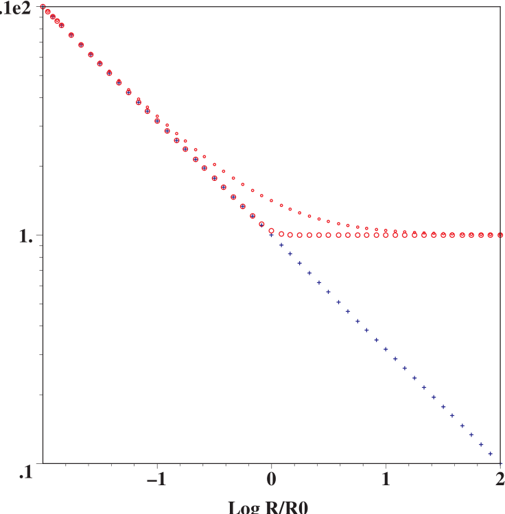
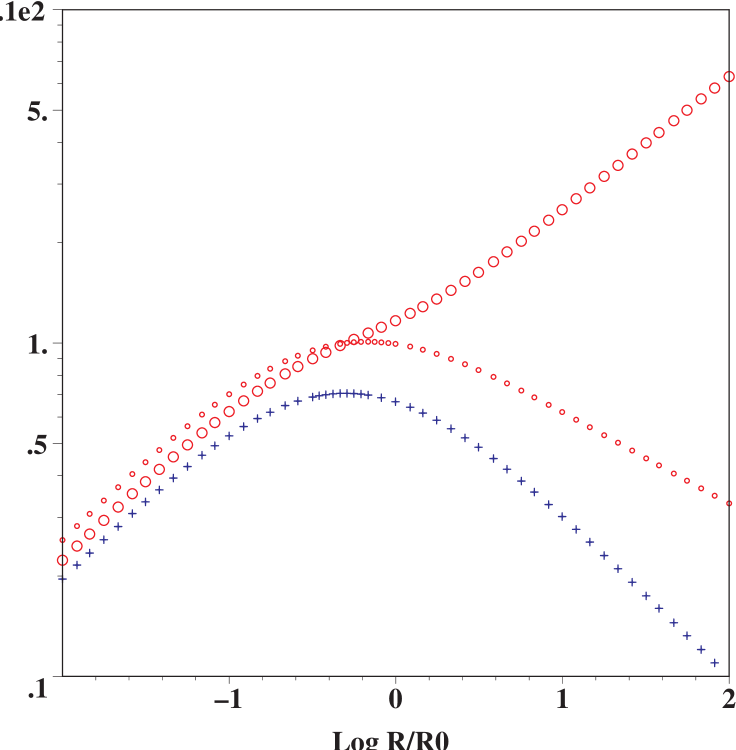
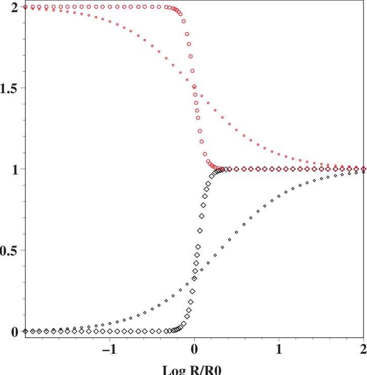
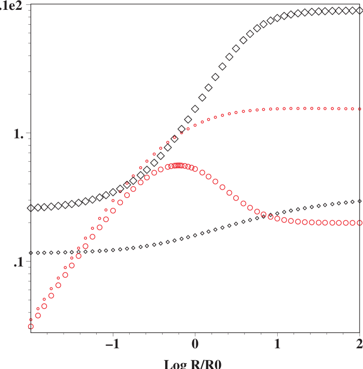
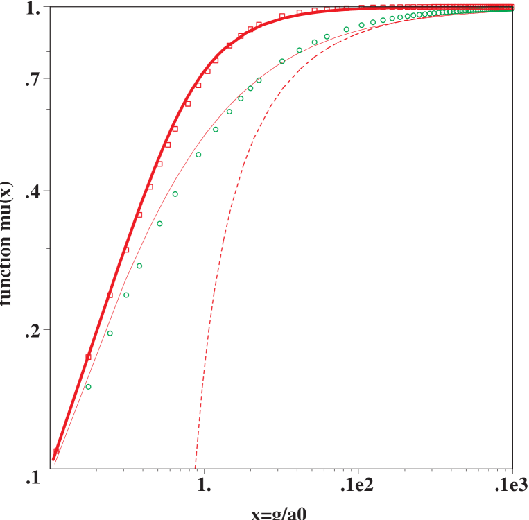
Figure 1: Top panels: shows the circular velocity curves $V_{\rm cir}(R)=\sqrt{gR}$ in various modified gravity (red circle) (cf. eq. 3) and $V_{\rm cir}(R)=\sqrt{g_{N}R}$ in Newtonian gravity (blue cross); both in units of $\left(GM_{0}a_{0}\right)^{1/4}$. These are shown in left panels for point mass with $(k,n)=(1/2,1)$ (smallest symbols), $(k,n)=(1/2,8)$ (bigger symbols) and in right panels for an extended Hernquist profile mass with a scale $b=1/2$ in a stronger-than-MOND gravity with $(k,n)=(9/10,1)$. Middle panels: Same parameters as in upper panels, except showing $\zeta$ (red circles) and $\Delta$ (black diamonds) as functions of rescaled orbital distance $R/R_{0}$. Bottom panel: compares the function $\mu(g)$ in the popular MOND models ($\mu(x)=x/\sqrt{1+x^{2}}$ in boxes, and $x/(1+x)$ in circles) with our function in the case $(k,n)=(1/2,3)$ (thick line) and $(1/2,3/2)$ (thin line) and $(1,1)$ (dashed line).

For more compact notations later on we shall introduce a few auxilary functions, related to $\mu$ in a spherical potential. We define

$$\Delta\left(g\right)\equiv{d\ln\mu\over d\ln g},\qquad\Delta_{1}\equiv\Delta+1={d\ln g_{\mu}\over d\ln g}.$$ (5)

We also define

$$\zeta(g)\equiv-\left({d\ln R(g)\over d\ln g}\right)^{-1}\!\!\!,\qquad\zeta_{1}\equiv\zeta+1=-{d\ln\Omega^{2}\over d\ln R},$$ (6)

where $\Omega(R)=\sqrt{g\over R}$ is the angular frequency for a circular orbit of radius $R$. In writing down $R(g)$ we treat the spherical radius $R$ as a function of the gravitational field strength $g$ through the relation $MR^{-2}\propto g_{N}\sim g_{\mu}=\mu g$. Note in the case of the field around a point mass, and assume non-negative $n$ and $k$, $\Delta(g)$ is related to the parameter $\zeta(g)$ by

$${\zeta\over 2}={d\ln g\over d\ln R^{-2}}={1\over\Delta_{1}}=\cases{1&near a point mass\cr 1-k&far from a point mass.\cr}$$ (7)

Conventional MOND models have the property that $(\Delta,\zeta)\rightarrow(0,2)$ when the gravity is strong and $(\Delta,\zeta)\rightarrow(1,1)$ when the gravity is much weaker than $a_{0}$. The result in this paper applies to any function $\Delta(g)$ or $\zeta(g)$. In general, we shall call the above gravity $g$ the MOND-like Gravity or Modified Gravity.

Fig. 1 shows how $\zeta$ (red circles) and $\Delta$ (black diamonds) change as the MONDian gravity decreases away from a point mass (middle left panel) and from an extended mass (middle right panel). These MOND models have a narrow range of $1\leq\zeta\leq 2$ or $1\geq\Delta\geq 0$.

3 Roche Lobes of a two-body system in a MOND-like gravity

A binary system is specified by two baryonic masses $M$ and $m$ separated by a distance $D_{o}$ along, say, the z-axis. The two bodies could be a galaxy and a satellite. The MOND-like gravity distribution is determined by equation (1) where $N=2$ for a binary. Define the inner Lagrange point of the binary at a distance $r_{1}$ and $D_{o}-r_{1}$ from the masses $m$ and $M$. There are only 3 independent dimensionless quantities in this system, $r_{1}/(D_{o}-r_{1})$, $m/M$ and a typical value for the parameter $\zeta$. From dimensional arguments we expect that the Roche radius might be expressable in general as

$${r_{1}\over D_{o}}=\left({m\over A(\zeta)M}\right)^{B(\zeta)},$$ (8)

where $A$ and $B$ are dimensionless functions with dimensionless arguments; we now go on to show, using perturbation analysis, that this is indeed the case, and we set the exact expressions for $A$ and $B$.

We set up the coordinate system such that the origin is on the smaller mass $m$, at a distance $D_{o}$ from the mass $M$ on the z-axis. Let the low-mass satellite with $m/M\ll 1$ rotate around the mass $M$ (fixed) with an angular velocity $\Omega\hat{\bf y}$, then particles in the corotating frame conserve the Jacobi energy with an effective (triaxial) potential

$$\Phi_{e}(x,y,z)\equiv\Phi-{x^{2}+(z-D_{o})^{2}\over 2}\Omega^{2},\leavevmode\nobreak\ \Phi\equiv\Phi_{0}+\Phi_{1},$$ (9)

where the gravitational potential $\Phi$ of the galaxy-satellite system is expressed as two terms, where we treat the effect of the smaller mass $m$ as a perturbation $\Phi_{1}$ to the unperturbed potential $\Phi_{0}$ of the bigger mass $M$.

First consider the unperturbed case where we set the satellite $m=0$. At a distance $R$ far way from the isolated baryonic mass $M$, the gravitational potential can in general be approximated as spherical with

$$\Phi_{0}=\int g(R)dR,\qquad R=\sqrt{(z-D_{o})^{2}+y^{2}+x^{2}}$$ (10)

where the gravity $g(R)$ at radius $R$ from the spherical galaxy centre is related to the Newtonian gravity $-GM{\bf R}/R^{3}$ by

$${\bf g}_{\mu}={\bf g}_{N}=-{GM\over R^{3}}[x,y,z-D_{o}],\qquad{\bf g}=-{\bf\nabla}\Phi_{0}(R).$$ (11)

Taylor-expand the three components of the gravity in the vicinity of the origin $(x,y,z)=(0,0,0)$, we have

$${\bf\nabla}\Phi_{0}\approx[x,y,D_{o}]\Omega^{2}+[0,0,z]{dg(D_{o})\over dD_{o}},\leavevmode\nobreak\ \Omega^{2}\equiv{g(D_{o})\over D_{o}}.$$ (12)

The gravity field is such that if a test particle is put on circular orbit with an orbital radius $R=D_{o}$ around $M$, then the rotation angular frequency must be $\Omega$ in order to balance gravity with centrifugal force. Integrate the above potential gradient, we find

$$\Phi_{0}(R)\approx\Phi_{0}(D_{o})+\left[x^{2}+y^{2}-z^{2}\zeta\right]{\Omega^{2}\over 2}+zD_{o}\Omega^{2}$$ (13)

in the vicinity of the origin $(0,0,0)$, where according to the definitions of $\zeta$ and $\Delta$ we have $\zeta=-{d\log g(D_{o})\over d\log D_{o}}$.

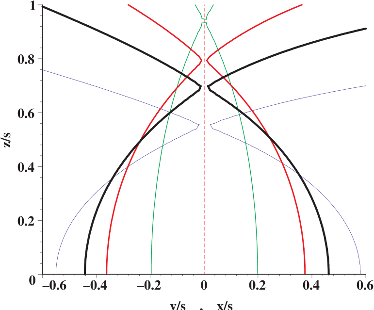
Figure 2: shows one octant of the 3-dimensional Roche Lobe of a satellite of mass m rotating in the xz plane around a mass M at a distance $D_{o}$ on the z-axis. The sizes are scaled by a length $s\equiv\left({m\over M(D_{o})}\right)^{1/3}D_{o}$. The curves are for $\zeta=-{d\ln g\over d\ln D_{o}}=2$ (Newtonian, thick black) and $\zeta=1$ (Deep-MOND, red). A slimer Roche lobe for $\zeta=1/5$ (thin green) and a fatter Roche lobe for $\zeta=5$ (thin blue) are also made for comparison.

Now we consider the perturbation due to the satellite. Milgrom (1986) showed that in a medium under a uniform external field $g_{0}\hat{z}$ with a dielectric index $\mu(g_{0})$, the perturbation due to the added point-mass $m$ is almost Newtonian apart from a mild anisotropy with a potential (cf. his eq. 11)

$$\Phi_{1}(x,y,z)=-{Gm^{\prime}\over\tilde{r}},\leavevmode\nobreak\ \tilde{r}=\sqrt{z^{2}+\Delta_{1}\left(y^{2}+x^{2}\right)},$$ (14)

where $m^{\prime}=m/\mu(g_{0})$ is the modified inertia of the point mass, and $\tilde{r}$ is the effective distance from the centre of the satellite and $\Delta_{1}=\Delta+1=1+{d\log\mu(g_{0})\over d\log g_{0}}\neq 1$ is the MOND dilation factor. Here we show that we can recover the same expression for a satellite in a galaxy. Sufficiently far away from the satellite, the gravity is dominated by the spatially slow-varying gravity field of the unperturbed galaxy, which we denote with the shorthand $g_{\bf R}\equiv|{\bf g}({\bf R})|$. We also use the shorthand $\mu_{\bf R}\equiv\mu(|{\bf g}({\bf R})|)$ to denote the slow-varying MOND ”dielectric index” due to the galaxy. The perturbed dielectric index is $\mu_{\bf R}$ plus a perturbation due to the self-gravity of the satellite, which is given by

$$\mu(|{\bf g}|)-\mu_{\bf R}\approx{d\mu\over dg}\left[|{\bf g}|-g_{\bf R}\right]\approx{d\mu\over dg}\hat{{\bf R}}\cdot{\bf\nabla}\Phi_{1}.$$ (15)

The perturbation part of the modified Poisson’s equation (eq. 1) becomes

$${\bf\nabla}\cdot{\mu_{\bf R}{\bf g}_{\bf R}\over 4\pi G}-{\bf\nabla}\cdot{\left(\mu_{\bf R}+{d\mu\over dg}{\bf\nabla}_{\bf R}\Phi_{1}\right)({\bf g}_{\bf R}-{\bf\nabla}\Phi_{1})\over 4\pi G}\approx m\delta(r).$$ (16)

Cancel out the 0th order terms due to the mass $M$ only, drop terms of order $|{\bf\nabla}\Phi_{1}|^{2}$ and small terms of order ${1\over R}{\bf\nabla}\Phi_{1}$, we end up with a linear equation for $\Phi_{1}$, which in the vicinity of the satellite is given by

$$\left(\Delta_{1}\partial_{z}^{2}+\partial_{x}^{2}+\partial_{y}^{2}\right)\Phi_{1}=4\pi Gm^{\prime}\delta(r),$$ (17)

where

$${Gm^{\prime}\over Gm}\approx{1\over\mu_{\bf R}}\approx{g(D_{o})\over g_{\mu}(D_{o})}={\Omega^{2}D_{o}\over GMD_{o}^{-2}}.$$ (18)

Apply the transformation $z^{\prime}=z\sqrt{\Delta_{1}}$, $x^{\prime}=x$, $y^{\prime}=y$, it can be shown that to the first order in $m$ the perturbation in potential is given by equation (14), where $g_{0}\approx g_{\bf R}\approx g(D_{0})$. As verified by Milgrom (1986) using a numerical solver, our equation (14) is ”a good approximation” as long as the Newtonian force of the satellite ${Gm\over r^{2}}$ is small compared to the Newtonian part of the external field $g_{0}\mu(g_{0})$, ”thus the equipotential surfaces are ellipsoids of revolution with the major axis in the direction of the external field.”

The combined potential $\Phi(x,y,z)=\Phi_{0}(R)+\Phi_{1}(x,y,z)$ clearly has axial symmetry around the z-axis, and has two centres separated by distance $D_{o}$ along the z-axis. The above formulation approximates the potential of, e.g., the Milky Way galaxy of baryonic mass $M$ plus a satellite of baryonic mass $m$.

The effective potential $\Phi_{e}(x,y,z)$, if Taylor expanded near the secondary $(0,0,0)$, has an triaxial shape with

$$\Phi_{e}\approx cst+\Omega^{2}D_{o}^{2}\left[{y^{2}-\zeta_{1}z^{2}\over 2D_{o}^{2}}-{D_{o}m/M\over\sqrt{z^{2}+\Delta_{1}(y^{2}+x^{2})}}\right],$$ (19)

where the terms to the first order of $z$ and second order to $x$ are canceled due to force balance. The inner or outer Lagrangian points is then calculated from the saddle point of the effective potential where

$$0=\left.{\partial\Phi_{e}(0,0,z)\over\partial z}\right|_{z=\pm r_{1}}=\Omega^{2}D_{o}\left[\mp{r_{1}\zeta_{1}\over D_{o}}\pm{m\over M}{D_{o}^{2}\over r_{1}^{2}}\right].$$ (20)

This definition of the Lagrange radius $r_{1}$ reduces to

$$\left({m\over r_{1}^{3}}\right)=\zeta_{1}\left({M\over D_{o}^{3}}\right).$$ (21)

So inside the Lagrange radius $r_{1}$ the average density of the satellite equals k-times the average density inside the orbital radius $D_{o}$ of the satellite. The equation can also be written as

$${r_{1}\over D_{o}}=\left({m\over\zeta_{1}M}\right)^{1\over 3},\qquad\zeta_{1}=1+\zeta.$$ (22)

Note that the masses here $m$ and $M$ are true baryonic masses of the binary, not the modified inertia masses. Eq. (21) can be further massaged into

$$\Omega^{\prime}\equiv\sqrt{Gm^{\prime}\over r_{1}^{3}}=\sqrt{\zeta_{1}}\Omega,$$ (23)

where $\Omega^{\prime}$ takes the meaning of the angular frequency of circulation around the secondary at its Robe radius. Hence the tidal radius of the secondary scales linearly with the terminal velocity of the secondary, and the internal period is within a factor of $\sqrt{\zeta_{1}}$ of the period of the secondary’s orbit. Finally note that near the tidal radius, the gravity due to the secondary and primary has the ratio

$${Gm^{\prime}\over r_{1}^{2}g(D_{o})}=\zeta_{1}\left({m\over M}\right)^{1\over 3}\ll 1,$$ (24)

which confirms that near the tidal radius $r_{1}$ it is valid to approximate the self-gravity of a low-mass secondary ($m/M\ll 1$) as a perturbation to the slow-varying gravity $g(D_{o})$ of the primary.

The shape of the Roche Lobe is specified by contour of equal effective potential with the contour passing the Lagrange points $(0,0,\pm r_{1})$. The effective potential can be redefined as a dimensionless function $\Psi_{e}(x,y,z)$ after massaging zero point and a prefactor. Substitute $(m/M)$ in favor of $r_{1}/D_{o}$ using eq. (22), we found that the points $(x,y,z)$ along the Roche lobe satisfy

$$\Psi_{e}={3\zeta_{1}r_{1}^{2}+y^{2}-\zeta_{1}z^{2}\over 2r_{1}^{2}}-{\zeta_{1}r_{1}\over\sqrt{z^{2}+\Delta_{1}y^{2}+\Delta_{1}x^{2}}}=0.$$ (25)

Clearly the z-axis intersects the Roche Lobe at $(0,0,\pm r_{1})$, where

$${r_{1}\over D_{o}}=\left({m\over\zeta_{1}M}\right)^{1\over 3},$$ (26)

which defines the first axis of the Roche Lobe. Draw a line parallel to the x-axis direction, it intersects the Roche lobe at $(\pm r_{2},0,0)$. Solving equation (25) we find

$${3r_{2}\over 2r_{1}}={1\over\sqrt{\Delta_{1}}},$$ (27)

which defines the second axis of the Roche Lobe. Likewise the third axis of the Roche Lobe is defined by the intersection points $(0,\pm r_{3},0)$ with a line parallel to the rotational y-axis. We find

$${2r_{3}\over 3r_{2}}=(u^{2}-1)^{1\over 3}\left[(u+1)^{1\over 3}-(u-1)^{1\over 3}\right],\leavevmode\nobreak\ u\equiv\sqrt{1+\Delta_{1}\zeta_{1}}$$ (28)

by simply solving equation (25), which reduces to an essentially cubic equation

$${r_{2}\over r_{3}}-1={4\over 27\Delta_{1}\zeta_{1}}\left({r_{3}\over r_{2}}\right)^{2}.$$ (29)

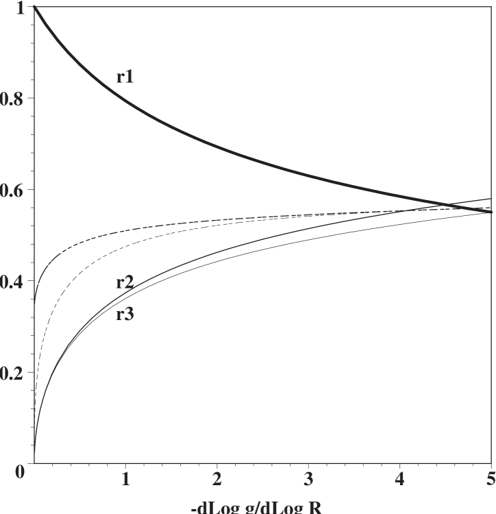
Figure 3: shows the Roche lobe semi-axis sizes $r_{1},r_{2},r_{3}$ of a satellite $m$ at orbital distance $R=D_{o}$ as functions of the gravity power-law index $\zeta=-{d\log g\over d\log D_{o}}$. Here the sizes are rescaled by $s\equiv\left({m\over M(D_{o})}\right)^{1/3}D_{o}$. Also shown are the arithematic mean $(r_{1}+r_{2}+r_{3})/3$ (thicker dashed curve), and the geometric mean size $|r_{1}r_{2}r_{3}|^{1/3}$ (thin dashed curve).

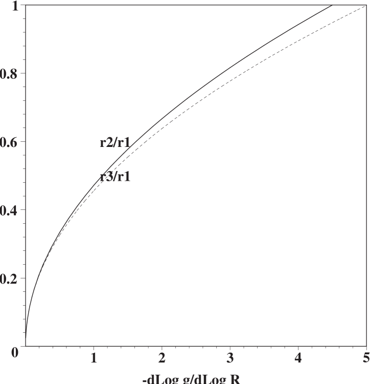
Figure 4: similar to the previous one, but shows the aspect ratio of the Roche lobe semi-axis sizes $r_{2}/r_{1},r_{3}/r_{1}$ as functions of $\zeta=-{d\log g\over d\log R}$.

4 Generalisation and Discussion

4.1 Extended spherical primary mass

Although we refer to our primary mass as a mass point, our result applies exactly for a spatially extended spherical mass distribution of the primary $M(R)$, e.g., a galaxy, if we simply make the substitution

$$M\rightarrow M(R).$$ (30)

As a result the $\zeta-\Delta$ relation changes to

$$2-{d\ln M\over d\ln R}=\zeta\Delta_{1}.$$ (31)

As a specific example, a host galaxy can be approximated by a spherical Hernquist mass profile with

$$M(R)=M_{0}\left({R\over R+y_{h}R_{0}}\right)^{2},\qquad R_{0}\equiv\sqrt{GM_{0}\over a_{0}},$$ (32)

with the scalelength parameter $y_{h}=1/2$, where we adopted notations of Zhao, Bacon, Taylor et al. (2005). The Newtonian gravity of the model is

$$g_{N}={GM(R)\over R^{2}}=a_{0}\left(y_{h}+y\right)^{-2},\qquad y\equiv{R\over R_{0}}.$$ (33)

Note $g_{N}=a_{0}/(1+b)^{2}=4a_{0}/9<a_{0}$ at $R=R_{0}$ and $g_{N}=a_{0}/b^{2}=4a_{0}$ is finite at $R=0$. We give the Hernquist model a stronger-than-MOND gravity with $(k,n)=(9/10,1)$ so that the model has a rising terminal velocity curve. As shown by Fig.1b this model has $\zeta=0$ near the primary, and $\zeta=1/5$ far away.

,

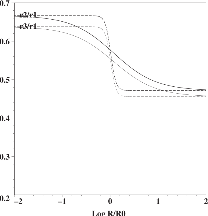
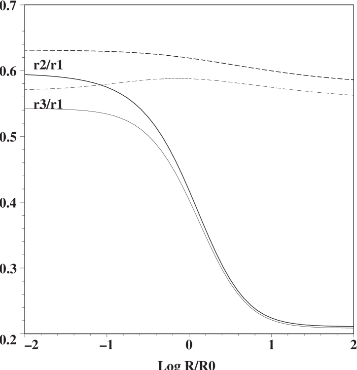
Figure 5: showing the Roche lobe axis ratios $r_{2}/r_{1},r_{3}/r_{1}$ as functions of $R/R_{0}$ with $R=D_{o}$ being the orbital distance of the secondary. Left panel: Models are as in Fig.1a and Fig.1c, with $(k,n)=(1/2,1)$ (solid) and $(k,n)=(1/2,8)$ (dashed). Right panel: as in Fig.1b and Fig.1d, with $(k,n)=(9/10,1)$ (solid) and $(k,n)=(1/4,1)$ (dashed) around a Hernquist profile mass.

4.2 Prolate or oblate?

Interestingly, the second and the third (i.e., rotation) axes of the Roche lobe are always very similar in length. This is because equation (29) contains a factor ${4\over 27\Delta_{1}\zeta_{1}}={4\over 27(\Delta+3)}\ll 1$ for any $-1<\Delta<\infty$. In fact that

$${r_{2}\over r_{3}}=[1,1.02,1.03,1.045,1.055,1.065]\approx 1,$$ (34)

for $\zeta=[0,0.5,1,2,4,\infty]$, where $\zeta=1,2$ are the deep-MOND, and deep-Newtonian cases.

The first axis is often substantially longer than the other two, but not always. We find for point masses

$${r_{1}\over r_{2}}=[\infty,3,2.12,1.5,0.95,0],\leavevmode\nobreak\ {\rm for\leavevmode\nobreak\ }\zeta=[0,0.5,1,2,5,\infty].$$ (35)

The generally triaxial Roche lobe for point masses is nearly prolate for $0<\zeta<5$, and it becomes nearly spherical for $\zeta=4-6$, and becomes nearly oblate only in exotic situations where the power-law index $\zeta=|d\ln g/d\ln R|$ is ”harder” than 5. For extended mass, the ratio can be calculated from

$${r_{1}\over r_{2}}={3\over 2}\sqrt{\Delta_{1}}={3\over 2}\sqrt{d\log g_{N}\over d\log g},$$ (36)

together with a relation between $g$ and $g_{N}$ (cf. eq. 3) and $g_{N}={GM(R)\over R^{2}}$.

Overall the Roche lobe axis ratio changes by a significant amount for different assumptions of the laws of gravity and the mass profile (cf. Fig. 5), e.g., the MONDian Roche lobe ($k=1/2$) at large distance is significantly more squashed than the Newtonian case, and a modified gravity with $k=9/10$ at large distance is even more squashed. We speculate that it might be feasible to differentiate these laws with a precise measurement of a Roche lobe. One advantage of using axis ratio is that it does not require precise knowledge of the satellite baryonic mass and its actual distance and absolute size; none of these factors enter equations (27) and (28). In particular we note that in Newtonian gravity $\Delta_{1}=1$, hence ${r_{1}\over r_{2}}={3\over 2}$ holds for any mass distribution at any distance; it would be interesting for testing non-Newtonian gravity to quantify the deviation from this ratio in observed Roche lobe.

,

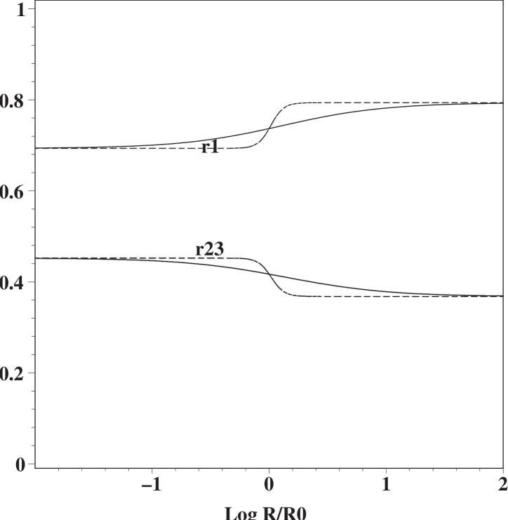
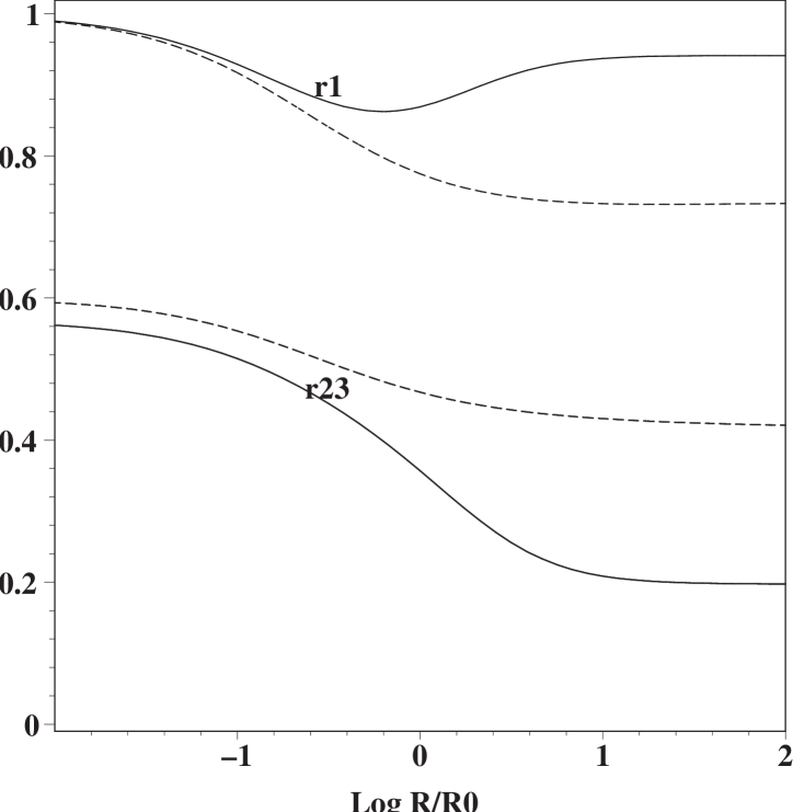
Figure 6: showing the Roche lobe semi-axis sizes $r_{1},\sqrt{r_{2}r_{3}}$ as functions of $R/R_{0}$. Here the sizes are rescaled by $s\equiv\left({m\over M(R)}\right)^{1/3}R$ with $R=D_{o}$ being the orbital distance of the secondary. Left panel: models as in Fig.1a and Fig.1c, with $(k,n)=(1/2,1)$ (solid) and $(k,n)=(1/2,8)$ (dashed). Right panel: models as in Fig.1b and Fig.1d, with $(k,n)=(9/10,1)$ (solid) and $(k,n)=(1/4,1)$ (dashed) around a Hernquist profile mass.

4.3 Size-mass and size-distance relations

In general, the Roche radii of two-body systems (whether stellar binaries or satellite-host galactic binaries) provide a measure of the relative weights of the binary in baryons in any MOND-like gravity. It is interesting that the Roche Lobe size in any MOND-like gravity has the same simple scaling relation

$${m\over r_{1}^{3}}/{M(D_{o})\over D_{o}^{3}}=\zeta_{1}=2-{d\log V_{\rm cir}^{2}\over d\log R}.$$ (37)

The above relation holds for an extended primary as well. As in the Newtonian case the relevant mass is the unmodified true baryonic mass of the binary, the difference is only in the prefactor, which depends on the $M$ and $D_{o}$. For point masses the prefactor varies from $\zeta_{1}=3$ in the region with Keplerian rotation $V_{\rm cir}\propto R^{-1/2}$ (Binney & Tremaine 1987) to $\zeta_{1}=2$ for the flat rotation curve region. A similar relation holds for $r_{2}$,

$$\Theta_{\rm IR}\equiv{r_{2}\over D_{o}}\left({m\over M}\right)^{-1/3}={2\over 3\Delta_{1}^{1\over 2}\zeta_{1}^{1\over 3}},$$ (38)

where

$$\zeta_{1}=2-{d\log V_{\rm cir}^{2}\over d\log R},\qquad\Delta_{1}={d\log g_{N}\over d\log g}.$$ (39)

Here $\Theta_{\rm IR}$ takes the meaning of a rescaled Roche lobe intermediate semi-axis.

The size of the lobe varies with the distance from the primary. The Roche Lobe sizes in terms of $r_{1}$ and $\sqrt{r_{2}r_{3}}\sim r_{2}$ can be read off from Fig. 6 for different assumptions of the $\mu$-function and mass profile; in practise we can treat the Roche lobe as prolate.

5 An application: Limiting radii of outer satellites of MW and M31

As an illustration of the usuage of the Roche lobe, we compare the predicted Roche sizes with the observed limiting radii of outer satellites of galaxies. Slightly different from Zhao (2005), the sample consists of all globular clusters and dwarf galaxies beyond 20 kpc (outside the disks) of both the Milky Way and Andromeda. Only Andromeda satellites with reliable 3-dimensional distances to the Andromeda centre are used (McConnachie et al. 2004); tidal radius and distance of the newly discovered AndIX are from Harbeck et al. (2005). The limiting angular radii $\theta_{\rm lim,min}$ are taken primarily from Harris (1996) and Mateo (1998). Most systems are consistent with no flattening in projection. For a few significant flattened systems we take the limiting radii on the minor axis. This radius should approximate the intermediate semi-axis $r_{2}$ of a nearly prolate Roche lobe if Roche lobes are filled; a prolate object appears the same width on the minor axis at any inclination angle. Hence we have

$${r_{2}\over D_{o}}=F_{1}^{-1/3}{D\over D_{\odot}}{D_{\odot}\over D_{o}}\theta_{\rm lim,min},\qquad F_{1}\leq 1,$$ (40)

where the factor $F_{1}\leq 1$ takes into the facts that (i) the Roche volume is smaller at the pericenter of an eccentric orbit of a satellite, and that (ii) the volume filling factor of the pericentric Roche lobe can still be less than unity if star counts drop below detection limit before reaching the edge of the lobe (e.g., Grebel et al. 2000). Several distances are involved here, $D_{o}$ is the present orbital distance, $D$ is the present distance of the Sun from the satellite, and $D_{\odot}$ is the Sun’s distance to the centre of the host galaxy (here the Milky Way or the Andromeda). The rhs is insensitive to errors on distance $D$; for the outer Milky Way satellites we have ${D\over D_{o}}\sim 1$, and for Andromeda satellites we have ${D\over D_{\odot}}\sim 1$. Assuming mass-tracing-light, we expect that the satellite-to-host mass ratio is the ratio $q_{*}$ of observable stars within a factor of two, allowing for some differences in age and metallicity. So we can define

$$F_{2}\equiv{m\over Mq_{*}}\sim 0.5-2.$$ (41)

Multiplying a factor $(m/M)^{-1/3}$ to both sides of the above equation (40), we have

$${r_{2}\over D_{o}}\left({m\over M}\right)^{-1/3}\sim F_{1}^{-1/3}\Theta_{\rm min}\leq\Theta_{\rm min},$$ (42)

where

$$\Theta_{\rm min}\equiv{D\over D_{\odot}}{D_{\odot}\over D_{o}}\theta_{\rm lim,min}q_{*}^{-1/3},$$ (43)

is an observable, taking the meaning of the rescaled limiting minor axis size of a satellite. If MOND-like mass-tracing-light models are correct, substitute in equations (26)and (27) we expect that

$$\Theta_{\rm min}\geq\Theta_{\rm IR}={2\over 3\Delta_{1}^{1\over 2}\zeta_{1}^{1\over 3}}\sim{2^{1/6}\over 3}=0.374,$$ (44)

where we used the fact that all the baryons are contained well inside 20kpc, and

$$\zeta_{1}=2-{d\log V_{\rm cir}^{2}\over d\log R}\sim 2,\qquad\Delta_{1}={d\log g_{N}\over d\log g}\sim 2,$$ (45)

Note that we do not have freedom in chosing the law of the gravity, or $\zeta_{1}$ or $\Delta_{1}$: they are all determined by the nearly flat circular velocity curves in the Milky Way and Andromeda, which are inferred from the fairly constant velocity dispersions of the outer satellites and other tracers of the outer halo such as PNe.

Satellites with known proper motions often suggest only mildly eccentric orbits: pericentric distances are rarely smaller than 1/2 of the present distances, and almost never smaller than 1/5 of the present distance (Dinescu et al. 1999, 2004 and references therein). Outer globulars on long period orbits also have time to fill the instantaneous Roche lobe by two-body relaxation (Bellazzini 2004). Globular clusters as a class generally exhibit extra-tidal stars under deep observations; a sharp break of the star count profile and/or sometimes two-dimensional confirmation of unvirialised structures outside the King radius have been shown for globular clusters in the Milky Way, Andromeda, and other galaxies (Leon, Meylan & Combes 2000, Lehmann & Scholz 1997, Sohn et al. 2003, Harris et al. 2002). To be generous we assume the instantaneous Roche lobe has a filling factor $F_{1}\sim 0.01-1$, or $F^{-1/3}\sim F_{1}^{-1/3}\sim 1-5$. So equation (44) predicts that the majority of satellites should lie in a band with dashed line boundaries as marked in Fig. 7.

In reality we observe a number of outliers to the inequality equation (44) and the expectation band. Overall we observe a very large scatter of $\Theta_{\rm min}$ for satellites in similar gravitational field with similar expected values of $\Theta_{\rm IR}$ (cf. Fig. 7). Our result depends on the uncertain orbital pericentres of the halo satellites. A better understanding of the issue will likely come with proper motions for a large sample of halo satellites from the GAIA astrometric mission.

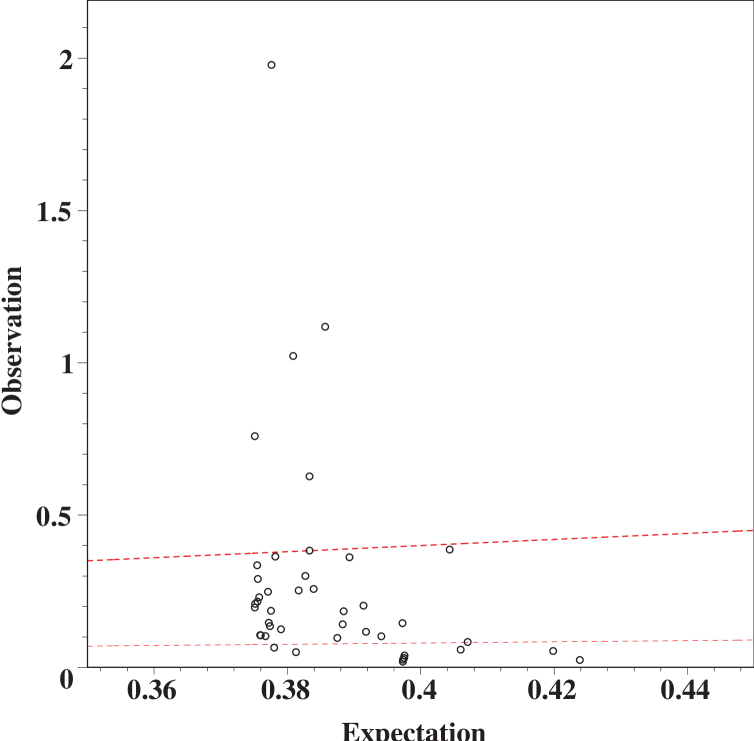
Figure 7: shows expectations vs. observations of the rescaled limiting minor axis radii $\Theta_{\rm min}$ of outer satellites (beyond 20kpc) of the Milky Way and Andromeda. The horizontal axis is the value of $\Theta_{\rm min}$ predicted from mass-tracing-light models assuming a satellite on a circular orbit filling its Roche lobe. The expectation band is shown by two slanted dashed lines; the expectation-observation equality line (thick diagonal dashed line) should be an upper limit for satellites are on eccentric orbits and not filling their Roche lobes. There are several outliers. To be conservative, we adopt a relatively low luminosity for the Milky Way and Andromeda so that $q_{*}={L_{\rm sat}\over 4\times 10^{10}L_{\odot}}$. To be accurate we adopt a slightly falling circular velocity curve $V_{\rm cir}=V_{0}\left[1+\left({r\over 100\,{\rm kpc}}\right)^{2}\right]^{-1/4}$ (cf. Wilkinson & Evans 1999) for the Milky Way and Andromeda.

6 Conclusion

The shapes of Roche lobes of a binary in a class of gravity theory including MOND are given analytically. The volume ratio of the Roche lobes is proven to scale linearly with the true mass ratio of the binary, hence models with dark matter would predict a Roche lobe volume $V$ times that predicted in mass-tracing-light models, where the factor $V=\left({M\over L}\right)_{\rm sat}\left({M\over L}\right)_{\rm host}^{-1}$ varies from $V\sim 1/10$ for typical outer globular clusters in a host galaxy to $V\sim 10$ for typical dwarf galaxies in a host galaxy. Observed limiting radii of outer satellites of the Milky Way have a large scatter, with some outliers by a factor of 4 above or factor 10 below predictions of our basic models for the Roche lobes in MOND-like mass-tracing-light gravity theories. The flattenings of the Roche lobe are independent of the mass ratio, but are sensitive to the function $\mu(g)$ in modifications to the law of gravity. Precise measurements of the exact shapes of other Roche-lobe-filling systems (e.g., mass-lossing stars or gas clouds in the outer halo of the Galaxy) might also test the law of gravity in the weak regime.

- (1) Baumgardt H., Grebel E.K., Kroupa P., 2005, MNRAS, 359, L1
- (2) Bekenstein J. 2004, Phys. Rev. D. 70, 3509
- (3) Bekenstein J., Milgrom M., 1984, ApJ, 286, 7,
- (4) Bellazzini, M. 2004, MNRAS, 347, 119
- (5) Binney J., Tremaine S., 1987, Galaxy dynamics, PUP
- (6) Brada R., Milgrom M. 2000, ApJ, 541, 556
- (7) Chiu M., Ko C.-M., Tian Y. 2005, ApJ in press, astro-ph/0507332
- (8) Ciotti L., Binney, J. 2004, MNRAS, 351, 285
- (9) Ciotti L., Londrillo P, Nipoti C. 2006, ApJ, in press (astro-ph/0512656)
- (10) Dinescu, D. I., Girard, T. M., and van Altena, W. F. 1999, AJ, 117, 1792
- (11) Dinescu D., Keeney B.A., Majewski S.R., Girard T.M., 2004, AJ, 128, 687,
- (12) Famaey B., Binney J. 2005, MNRAS, 363, 603
- (13) Grebel E., Odenkirchen M., Harbeck, D., 2002, AAS, 200, 4607
- (14) Hao J., Akhoury R. 2005, astro-ph/0504130
- (15) Harbeck D., Gallagher J.S., Grebel E.K., Koch A., Zucker D.B. 2005, ApJ, 623, 159
- (16) Harris, W. E., 1996, AJ, 112, 1487
- (17) Harris W.E., Harris G.L.H., Holland S.T., McLaughlin D.E. 2002, AJ, 124, 1435
- (18) Leon S., Meylan G., Combes F., 2000, A&A 359, 907
- (19) Lehmann I., Scholz R.D. 1997, A&A, 320, 776
- (20) Mannheim P., 1997, ApJ, 479, 659
- (21) Mateo M., 1998, ARA&A, 36, 435
- (22) McConnachie A.W., Irwin, M., Ibata R., Ferguson A. , Lewis G., Tavir N. 2004, MNRAS, submitted,
- (23) McGaugh S., 2005, Phys. Rev. Lett, 96, q1302
- (24) Milgrom M. 1983, ApJ, 270, 365
- (25) Milgrom M., 1986, ApJ, 302, 617
- (26) Milgrom M. , Sanders R. H. 2003, ApJ, 599, L25,
- (27) Pointecouteau E., Silk J., 2005, MNRAS, 364, 654
- (28) Qin B., Pen U., Silk J. 2005, Phy. Rev. Lett. submitted (astro-ph/0508572)
- (29) Qin B., Wu X.P., Zou, L.Z., 1995, A&A, 296, 264
- (30) Read J.I., Moore B. 2005, MNRAS, 361, 971
- (31) Sanders R., 3rd Aegean Summer School, The Invisible Universe: Dark Matter and Dark Energy, (astro-ph/0601431)
- (32) Sanders, R. , McGaugh S. 2002, ARA&A, 40, 263,
- (33) Skordis C., Mota D.F., Ferreira P.G., Boehm C., astro-ph/0505519
- (34) Sohn Y. et al. 2003 AJ, 126, 803
- (35) Sellwood J.A., Kowsowsky A. 2001, astro-ph/0009074
- (36) Sellwood J.A., Kowsowsky A. 2002, astro-ph/0109555
- (37) Wilkinson M., Evans N.W. 1999, MNRAS, 310, 645
- (38) Zhao H.S, 2005, astro-ph/0508635
- (39) Zhao H.S, 2005, A&A Letters, in press (astro-ph/0511713)
- (40) Zhao H.S., Bacon D., Taylor A.N., Horne K.D., 2006, MNRAS, in press (astro-ph/0509590)
- (41) Zhao H.S, Famaey B. 2006, ApJ Letters, in press (astro-ph/0512425)