A Principal Component Analysis approach to the Star Formation History of elliptical galaxies in Compact Groups

Abstract

Environmental differences in the stellar populations of early-type galaxies are explored using principal component analysis (PCA), focusing on differences between elliptical galaxies in Hickson Compact Groups (HCGs) and in the field. The method is model-independent and purely relies on variations between the observed spectra. The projections (PC1,PC2) of the observed spectra on the first and second principal components reveal a difference with respect to environment, with a wider range in PC1 and PC2 in the group sample. We define a spectral parameter ($\zeta\equiv 0.36$PC1$-$PC2) which simplifies this result to a single number: field galaxies have a very similar value of $\zeta$, whereas HCG galaxies span a wide range in this parameter. The segregation is found regardless of the way the input SEDs are presented to PCA (i.e. changing the spectral range; using uncalibrated data; subtracting the continuum or masking the SED to include only the Lick spectral regions). Simple models are applied to give physical meaning to the PCs. We obtain a strong correlation between the values of $\zeta$ and the mass fraction in younger stars, so that some group galaxies present a higher fraction of them, implying a more complex star formation history in groups. Regarding “dynamically-related” observables such as $a_{4}$ or velocity dispersion, we find a correlation with PC3, but not with either PC1 or PC2. PCA is more sensitive than other methods based on a direct analysis of observables such as the structure of the surface brightness profile or the equivalent width of absorption lines. The latter do not reveal any significant variation between field and compact group galaxies. Our results imply that the presence of young stars only amounts to a fraction of a percent in its contribution to the total variance, reflecting the power of PCA as a tool to extract small variations in the spectra from unresolved stellar populations.

1 Introduction

The connection between mass assembly and star formation provides the best approach to building a comprehensive picture of galaxy formation. In this respect, massive elliptical galaxies are ideal probes since their light is mostly dominated by old stellar populations, whereas their mass and morphology require late assembly. Both old ages and late assembly can be reconciled within the standard concordance cosmology. However, we currently lack a method to give an accurate estimate of the star formation history (SFH) from photo-spectroscopic data.

There are various factors that contribute to “decouple” the evolution of the total and stellar mass content of a galaxy. Most notably, the effect of feedback on star formation can make these two components follow divergent paths: for instance, a highly efficient mechanism of star formation at early stages can lead to “dry mergers” at later times (Bell et al. 2004). Indeed, the so-called downsizing trend (see e.g. Cowie et al. 1996; Treu et al. 2005) – in which lower mass galaxies contain most of the global star formation at later times – supports this effect.

The environment is another factor which can play an important role in shaping the SFHs of galaxies. Clusters of galaxies trace high density regions that collapsed earlier and present galaxies with a “hostile” environment in which gas can be removed by, for instance, ram pressure, galaxy harassment, and tidal interaction (e.g. Haynes 1989). Furthermore, the high virial velocities in clusters prevent mergers from taking place. This effect is dependent on the cosmic epoch and might be a non-trivial one to accurately estimate. The association between compact groups (CGs) and clusters has been investigated by Rood & Struble (1994) who find that 75% of Hickson’s groups seem to be associated to structures such as loose groups and clusters, indicating that CGs are actually part of the same observed hierarchy from isolated galaxies to superclusters. More recently, de Carvalho et al. (2005) examining a sample of CGs at a slightly larger redshift than Hickson’s find that there is an excess of CGs within one Abell radius of the nearest cluster, over a random distribution (32%). Moreover, they find a marginal excess of CGs related to rich clusters relative to poor clusters, which might be important for considering properly the environment where CGs live in. Therefore, it is of paramount importance to establish the connection between CGs and the large scale structure. In this context, it is important to remember that groups are the dominant type of structure found in the Universe (Nolthenius & White 1987) making them especially important from the cosmological viewpoint.

The effects of the environment on the galaxian properties have been studied over more than two decades (Guzman et al 1991; de Carvalho & Djorgovski 1992) and the issue is still debatable. Recent work regarding differences between early-type galaxies with respect to environment have found controversial results. While some indicate that environment does play some role (de Carvalho & Djorgovski 1992; Ziegler et al. 2005), others find no difference at all (e.g. de la Rosa et al 2001a; Bernardi et al. 1998). Also, studies of the stellar population of early-type systems indicate that they are older and and more metal poor in compact groups and clusters than in the field (Rose et al. 1994; Proctor et al. 2005; de la Rosa et al. 2001b; Mendes de Oliveira et al. 2005), suggesting that Es in dense systems experience a truncated period of star formation, which ultimately affects their chemical enrichment history, as opposed to their counterparts in the low density regime.

This paper presents an alternative approach to the analysis of unresolved old stellar populations, focused towards a comparison of the star formation history between CGs and the field. The current epoch of large surveys provides a fertile ground for statistical techniques such as PCA (Madgwick et al. 2002), ICA (Lu et al. 2006), IB (Slonim et al. 2001) or ANNs (Naim et al. 1995). We show here the capabilities of PCA to disentangle the star formation history of early-type galaxies. The structure of the paper is as follows: §2 presents the sample, §3 explains the technique of principal component analysis applied to spectra. §4 gives the results for our sample, which are put in context with physical models in §5, followed by a discussion in §6.

2 The sample

Our sample comprises 30 elliptical galaxies split into 18 located in the cores of Hickson Compact Groups (HCGs; Hickson 1982), and a control set of 12 early-type galaxies located either in the field, in the outskirts of clusters or in very loose groups. The sample selection criteria and spectroscopic data is presented in de la Rosa, de Carvalho & Zepf (2001a). The main details of the sample are listed in table 1. All galaxies were observed with the same instrument and configuration: long-slit spectroscopy over the 3500–7000Å range, with a FWHM resolution of 4.25Å . We removed from the original sample four galaxies (HCG 28b; 37e; 46a; 59b) since they have rather low signal-to-noise ratios. The remaining galaxies in the sample have S/N$\lower 2.15277pt\hbox{$\;\buildrel>\over{\sim}\;$}35$Å^-1. The extraction aperture was chosen to encompass all available flux (de la Rosa et al. 2001a). Flux calibration was performed by a comparison with standard stars observed during the same run and with the same configuration. Three standard stars were used: Hiltner 600 (B3), HZ44 (B2) and Feige 34 (DA). Comparing the flux-calibrated spectra using independently these stars, we get discrepancies in flux up to 7%.

The SEDs were dereddened using the Fitzpatrick (1999) $R_{v}=3.1$ Galactic extinction curve, taking the reddening values from the maps of Schlegel, Finkbeiner & Davis (1998) as shown in table 1. Notice that the reddening values between group and field sample span a similar range.

Table 1: Group and Field sample

Galaxy	Type	$M_{B}$	$\log\sigma_{0}$	E(B$-$V)	PC1a	PC2a	PC3a	$\langle a_{4}/a\rangle$	[Mg/Fe]b
		($h=0.7$)	(km s-1)		$\times 10^{3}$	$\times 10^{4}$	$\times 10^{4}$	$\times 100$
COMPACT GROUP GALAXIES
HCG 10b	E1	$-21.40$	2.388	0.051	5.214	1.934	0.221	0.164	0.24
HCG 14b	E5	$-20.42$	1.983	0.025	6.002	$-$1.885	0.924	0.577	0.45
HCG 15b	E0	$-20.25$	2.139	0.029	5.899	0.504	1.072	—	—
HCG 15c	E0	$-20.74$	2.209	0.029	5.676	1.797	0.242	$-$0.023	0.24
HCG 19a	E2	$-22.56$	2.262	0.033	5.897	$-$0.051	0.641	0.737	0.26
HCG 32a	E2	$-22.32$	2.278	0.091	7.007	$-$4.092	0.153	0.429	0.25
HCG 37a	E7	$-21.59$	2.420	0.031	6.269	$-$1.379	0.026	$-$0.535	0.21
HCG 40a	E3	$-21.48$	2.381	0.065	5.897	0.154	0.085	1.198	0.24
HCG 44b	E2	$-19.74$	2.263	0.025	4.785	2.181	0.817	0.274	0.16
HCG 46c	E1	$-19.17$	1.980	0.032	6.795	$-$6.819	0.747	0.497	—
HCG 51a	E1	$-21.20$	2.250	0.017	6.064	0.057	$-$7.783	$-$0.006	0.29
HCG 57c	E3	$-20.86$	2.339	0.031	6.415	$-$1.068	0.255	0.823	0.17
HCG 57f	E4	$-20.98$	2.152	0.031	6.730	$-$2.685	0.337	0.538	0.20
HCG 62a	E3	$-20.98$	2.326	0.052	5.560	0.056	0.298	$-$0.106	—
HCG 68b	E2	$-20.39$	2.205	0.011	5.392	$-$0.129	$-$0.533	$-$0.887	0.17
HCG 93a	E1	$-21.87$	2.372	0.136	5.110	1.410	0.427	$-$0.289	0.24
HCG 96b	E2	$-20.00$	2.298	0.059	5.147	1.302	1.057	0.458	0.16
HCG 97a	E5	$-21.09$	2.134	0.035	5.944	$-$1.478	$-$0.736	$-$0.004	0.09
FIELD GALAXIES
NGC 221	E2	$-17.42$	1.904	0.062	4.761	1.454	1.152	—	$-$0.04
NGC 584	E4	$-20.63$	2.295	0.042	5.105	1.771	0.204	0.29	0.24
NGC 636	E3	$-19.66$	2.209	0.026	5.478	0.924	0.592	0.07	0.16
NGC 821	E6	$-20.58$	2.282	0.110	5.056	1.920	$-$0.113	1.16	0.26
NGC 1700	E4	$-21.80$	2.378	0.043	5.694	0.664	0.154	0.48	0.15
NGC 2300	SA0	$-20.87$	2.397	0.097	5.261	0.194	$-$0.263	$-$0.39	0.39
NGC 3377	E5	$-19.17$	2.132	0.034	5.546	0.691	0.584	0.81	0.22
NGC 3379	E1	$-20.57$	2.304	0.024	5.043	2.032	$-$0.008	0.08	0.26
NGC 4552	E0	$-20.81$	2.386	0.041	5.092	1.343	0.092	0.02	—
NGC 4649	E2	$-21.54$	2.493	0.026	4.842	1.759	$-$0.586	$-$0.41	—
NGC 4697	E6	$-20.97$	2.211	0.030	5.208	1.438	0.334	1.04	0.14
NGC 7619	E2	$-21.86$	2.462	0.080	4.561	1.764	0.243	0.24	0.29

^a The PCs correspond to the calibrated SEDs in the $3800-4200$Å range.

^b Measured within R${}_{e}/2$.

Figure 1: First three principal components of the analysis for the flux calibrated data (left) and the continuum subtracted SEDs (right). Notice $\vec{e_{1}}$ and $\vec{e_{2}}$ map the average old populations and a younger stellar component, respectively.

3 Principal Component Analysis

In order to find systematic differences in the stellar populations of group and field ellipticals we apply principal component analysis (PCA) to the spectral energy distributions in various ways (Throughout this paper, the spectra are given as photon flux: F($\lambda$)). PCA is a model-independent method which aims at extracting those linear combinations of the data with the highest variance. Stellar spectra were the first astrophysical data on which principal component analysis was applied (Deeming 1964). PCA has been extensively used in the analysis of spectra from quasar and galaxy surveys (e.g. Francis et al. 1992; Connolly et al. 1995; Folkes, Lahav & Maddox 1996; Madgwick et al. 2002; Yip et al. 2004). This technique is ideal for our purposes. Regardless of the responsible physical mechanisms, we want to find in a robust way systematic differences between the stellar populations in group and field elliptical galaxies. Eventually, we compare our results with simple models of galaxy formation to give physical meaning to these differences.

Our application of PCA is as follows: We have 30 spectra $\Phi_{i}(\lambda)$ ($i=\{1\cdots 30\}$) which are defined at a number of discrete wavelengths $\lambda_{j}$ ($j=\{1\cdots N\}$). The spectra are normalized to the same flux integrated along the wavelength region of interest. PCA consists of diagonalizing the covariance matrix:

$$C_{jk}=\frac{1}{30}\Sigma_{i=1}^{30}\Phi_{i}(\lambda_{j})\Phi_{i}(\lambda_{k})\hfil 1\leq j,k\leq N,$$ (1)

so that the eigenvectors ($\{\vec{e}_{i}\}$) corresponding to the largest eigenvalues ($\{\nu_{i}\}$) will carry most of the information in these spectra. Notice that other methods use a different definition for the covariance matrix, most commonly including a subtraction of the average of the spectra of all galaxies at each wavelength (see e.g. Ronen, Aragón-Salamanca & Lahav 1999). This can be motivated if the observed spectra suffer from strong flux calibration uncertainties. Our sample, albeit small, has an accurate flux calibration which allows us to include the information from the continuum. We have performed tests of the other approach, namely subtracting the mean from the SEDs, and we find that this method roughly corresponds to “promoting” PC2 to PC1, etc. The correlations found are unaffected. Henceforth we present results based on PCA without mean subtraction.

One can use the eigenvectors as a basis, so that the components which correspond to the highest $\nu_{i}$ will carry most of the information. It is customary to sort the eigenvectors in decreasing order of their eigenvalues, and to express these ones as a fractional variance: $\nu^{\prime}=\nu_{i}/\Sigma_{j}\nu_{j}$. If the data can be simplified in a lower dimensional basis, PCA gives a small number of eigenvectors carrying most of the variance.

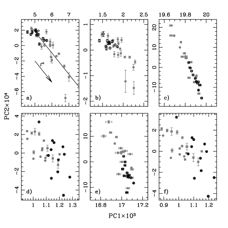
Figure 2: Projection of the observed SEDs on the first and second principal components. HCG and field galaxies are shown as grey dots and open circles, respectively. Each panel corresponds to: a) Calibrated SEDs straddling the 4000Å break in the 3800-4200Å range; b) Same as the previous one, using uncalibrated SEDs; c) Calibrated SEDs over a wider range of wavelengths: 3800–6000Å ; d) Continuum-subtracted SED; e) Only use the spectral range used by the Lick indices on the total SED; f) Same as e) applied to the continuum-subtracted SED. In all cases there is a clear segregation between group and field elliptical galaxies. $1\sigma$ error bars shown.

Figure 1 shows the first three eigenvectors (called principal components: $\vec{e_{1}}$, $\vec{e_{2}}$, $\vec{e_{3}}$) for two choices of spectra: The left panels are the principal components obtained when using the full, flux-calibrated SED. The panels on the right are those for continuum-subtracted spectra. The first principal component corresponds to an old stellar population. As expected, $\vec{e_{1}}$ carries most of the information that can be gathered from an elliptical galaxy, namely a prominent 4000Å break and strong absorption lines. The second eigenvector, $\vec{e_{2}}$, gives the next order of information in our sample, and clearly corresponds to a younger stellar component. The third component is noisier, but presents a remarkable feature at $\lambda=5170-5175$Å , corresponding to magnesium absorption. One should not interpret these SEDs too closely: the emission spike at the wavelength of the sodium feature ($\lambda=5890-5896$Å ) is just an artifact caused by the imposed orthogonality of the basis vectors.

Notice that, in contrast to studies applied to surveys of the entire galaxy population (e.g. Madgwick et al. 2003), our sample only comprises early-type galaxies. Hence, most of the information (which will be represented by the first principal component) corresponds to old stellar populations. Indeed, the normalized eigenvalues for those $\vec{e_{1}}$, $\vec{e_{2}}$, and $\vec{e_{3}}$ shown in the left panels of figure 1 are $\nu^{\prime}_{1}=0.9943$, $\nu^{\prime}_{2}=0.0013$ and $\nu^{\prime}_{3}=0.0007$. This implies that more than 99% of the information is carried by the first principal component, a result consistent with the findings of Eisenstein et al. (2003) on a sample of $22,000$ luminous early-type galaxies from SDSS. This is an “elegant way” to show that elliptical galaxies are dominated by old stellar populations. The aim of this paper is to explore PCA as a way of extracting small contributions from younger populations.

In order to robustly determine whether the star formation history of group and field elliptical galaxies differ in a significant way, we have to take into account possible systematic effects. Flux calibration errors introduce a smooth large-range variation in the SEDs, possibily mimicking effects of age or metallicity. In order to explore this effect, we applied PCA to “variations” of the spectral data. Figure 1 shows two such variations, namely the full, calibrated SED (left) and a continuum subtracted one (right). We also considered a reduced spectral range straddling the 4000Å break (3800–4200Å) thus minimising the effect of a flux-calibration error. Furthermore, we applied PCA to the raw, uncalibrated, unreddened data in this shorter spectral range. All SEDs were taken with the same instrument under the same configuration. Hence, we would expect raw data to carry the safest information about intrinsic differences among SEDs. The continuum-subtracted SEDs were obtained by subtracting the boxcar-smoothed spectrum using a 150Å window. Finally, we applied PCA to two sets of SEDs in which only the spectral regions targeted by the Lick indices (Trager et al. 1998) were considered. The wavelengths outside of both central and sidebands were masked out. These indices were specifically targeted to isolate the spectral regions which are most sensitive to age or metallicity. After masking out the other regions, we expect to reduce noise in the final results. This technique was applied both to the flux-calibrated SED and to the continuum-subtracted spectra, as discussed in the next section.

4 Results

Figures 2 and 3 show the results for the various methods given above. Once the covariance matrix is diagonalised, we project the observed SEDs on the first three principal components. For instance, the first component of the $ith$ galaxy is computed in the following way:

$$PC1_{i}=\vec{\Phi}_{i}\cdot\vec{e}_{1}=\sum_{j=1}^{N}\Phi_{i}(\lambda_{j})e_{1}(\lambda_{j}).$$ (2)

These projections correspond to the values shown in the figures as PC1, PC2 and PC3. Given that PCA diagonalises the covariance matrix, it is invariant with respect to a sign change in the projections, e.g. $\vec{e}_{2}$ and $-\vec{e}_{2}$ are equally valid eigenvectors. We fix this by choosing the sign that always results in an anticorrelation between PC1 and PC2. In order to compute the uncertainty in the principal components, we follow a Monte Carlo method: For each galaxy we generate 100 spectra by adding noise compatible with the observed S/N. Each set of “noisy” SEDs is presented to PCA and the projected value for each galaxy from these 100 realisations is used to determine the error bars, quoted throughout this paper at the $1\sigma$ level. Notice that the projections of the higher-order principal components are much smaller, which reflects the amount of information (in the sense of variance) carried by each of these first three components. The remaining higher-order components are noisier and we do not include them in this analysis. In fact, PCA has filtered the data so that most of the information from each spectrum can be reduced to three numbers, namely PC1, PC2 and PC3. Throughout this paper galaxies belonging to Hickson Compact Groups are represented as grey filled dots, whereas the field sample is shown as open circles.

4.1 Integrated SEDs

Figures 2 and 3 correspond to the integrated spectra from each galaxy, i.e. we only explore galaxy-to-galaxy variations, without any spatial resolution. Figure 2 shows a remarkable segregation between the group and field sample for all possible choices of SEDs used: a) flux-calibrated and de-redenned SED in the 3800–4200Å range; b) raw data in the same spectral range; c) flux-calibrated and de-reddened SED in the 3800–6000Å range; d) Continuum-subtracted SED; e) “Lick masking” applied to the flux-calibrated data; f) “Lick masking” applied to the continuum-subtracted SEDs. All different techniques give a similar segregation in the PC1–PC2 plane. Field galaxies populate a much smaller range of values of PC1 and PC2 compared to group galaxies. The strong correlation between PC1 and PC2 gives a hint of the importance of these two components as seen in figure 1. PC1 represents old stellar populations, whereas PC2 tracks younger stars. PCA unfortunately cannot be used to determine the “physics” behind the correlation, but we will see below that this trend is expected from stellar evolution. The top left panel of figure 2 also shows the best linear fit to the correlation found between PC1 and PC2. We can then rotate the coordinate system, so that one of the axis carries most of the information. This rotated axis defines a spectral parameter $\zeta$ similar to the $\eta$ parameter in Madgwick et al. (2002). However, we must emphasize that the SEDs used in that case correspond to a wide range of morphologies and the mean had to be subtracted in order to minimise uncertainties in flux calibration. The connection between $\zeta$ and stellar populations is discussed in §5.

Figure 3 shows that PC3 is a rather noisy component (as well as the higher order ones). Hence, most of the information is carried by the first and second principal components, and we will concentrate hereafter on these two. Notice that HCG 51a is shown as an arrow in panels a, b,d and f, being an outlier with high values of PC3 compared to the rest of the sample. HCG 46c also appears as an outlier in panel b. Panels d and f – which correspond to continuum-subtracted spectra – show a segregation, with the field sample featuring a significantly narrower spread in PC3.

4.2 SEDs in apertures

The single slit spectra used so far – obtained over an aperture that maximises the flux available – have very high S/N, enabling us to extract SEDs in smaller apertures. Figure 4 presents the results of PCA applied to four different apertures chosen with respect to the half-light radius of each galaxy. These PCs correspond to the analysis of the 3800–4200Å flux-calibrated data, but the other methods give similar results. The data show a very similar segregation as in the integrated case, and no significant differences are found with respect to the choice of aperture. Hence, environmental differences appear to be related to a global factor. This result is to be expected if we assume that the formation timescale is short compared to their stellar ages. The small evolution found in the colour gradients of elliptical galaxies with redshift suggest these gradients are mostly a metallicity effect (Tamura & Ohta 2000; Ferreras et al. 2005). Furthermore, integral field unit spectroscopy targeting age-sensitive spectral features such as Balmer absorption show a rather homogeneous structure in kinematically distinct components (Davies et al. 2001, however see McDermid et al. 2005). Our results reveal that the differences between group and field early-type galaxies are global and do not relate to significant differences in their gradients.

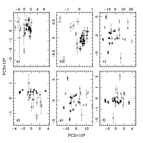
Figure 3: Projection of the sample SEDs on the second and third principal components. Group and field galaxies are shown as grey dots and star, respectively. The panels correspond to the same cases as in figure 2. Arrows are shown for a couple of galaxies which appear as outliers: HCG 51a in panels a,b,d,f and HCG 46c in panel b.

4.3 Structural parameters

Structural differences should be expected between group and field galaxies. The higher density but low velocity dispersions found in compact groups favour an increased interaction or merger rate among galaxies. Hence, elliptical galaxies in the cores of HCGs should reveal dynamical signatures from recent encounters (Proctor et al. 2004; Coziol et al. 2004)

We measured their isophotal shapes with the IRAF ELLIPSE routine (Jedrzejewski 1987) on the survey images acquired by Hickson (1994) in the $R$ band with the 3.6m Canada-France-Hawaii Telescope (CFHT). These images are publicly available on the NASA/IPAC Extragalactic Database (NED). ELLIPSE allows the isophote center, ellipticity and position angle to vary at each iteration. Once a satisfactory fit is found, it computes the sin and cos 3$\theta$ and 4$\theta$ terms, which describe the deviations of the isophotes from pure ellipses by means of the following Fourier expansion:

$$\begin{array}[]{cc}\Delta r(\theta)/r(\theta)=&(a_{3}/a)\cos(3\theta)+(a_{4}/a)\cos(4\theta)+\\ &\\ &+(b_{3}/b)\sin(3\theta)+(b_{4}/b)\sin(4\theta),\end{array}$$ (3)

where $\theta$ is the position angle, $r$ the distance from the galaxy centre and $a$ and $b$ the semi-major and semi-minor axes. The $a_{4}/a$ and $a_{3}/a$ parameters, where $a$ is the semi-major axis of the isophote, measure the deviations of the isophote from a pure ellipse. In particular, $a_{4}/a$ measures the deviations which are symmetric with respect to the galaxy center (i.e. found along the isophote every $90^{o}$). Positive (negative) values are obtained for disky (boxy) galaxies. Simulations show that boxy galaxies are remnants of massive mergers, whereas disky ellipticals are related to a larger mass difference between the merged progenitors (cf. Khochfar & Burkert 2005, Jesseit et al. 2005).

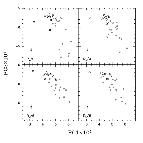
Figure 4: The first two principal components are shown taking the 3800-4200Å spectral range for different apertures, chosen with respect to the half-light radius of each galaxy. A characteristic error bar is shown

We ran ELLIPSE on the images taken in the $R$ filter, leaving as free parameters the position of the centre, the ellipticity (defined as $1-b/a$, where $a$ and $b$ are the projected major and minor axes) and the position angle of the major axis and assuming a logarithmic step along the semi-major axis. We computed the average $\langle a_{3}/a\rangle$ and $\langle a_{4}/a\rangle$ parameters of each galaxy following the prescriptions of Bender et al. (1988) and in the R filter. The method in question consists of averaging the $a_{3}/a$ and $a_{4}/a$ values measured at R${}_{i}\leq r\leq$R_o weighted by their errors and by the counts in the isophote at each isophotal mean radius $r$. Here, R_o is 1.5 times the half-light radius (R_e) derived from the surface brightness radial profile and R_i is the radius corresponding to 3 times the FWHM of the PSF in the $R$ filter – FWHM(PSF)$\simeq 4$ pixels hence $1.6^{\prime\prime}$. The resulting mean values $\langle a_{4}/a\rangle$ are reported in table 1, together with the mean isophotal parameters of the field galaxies taken from Bender et al. (1988, 1989).

Figure 5 compares PC1, PC2 and PC3 with the structural parameter $a_{4}$ described above. The number of galaxies is too small to draw statistically significant conclusions. Most of the galaxies have either disky or very close to elliptical isophotes, although the ones with the highest values of PC1 and PC2 – which are mostly group galaxies – feature disky isophotes. PC3 presents a more significant correlation, an issue which is explored below in connection with velocity dispersion.

4.4 [Mg/Fe] abundance ratios and velocity dispersion

Abundance ratios such as [Mg/Fe] are very sensitive tracers of the duration of star formation. Magnesium is an alpha element, mainly produced in core-collapse supernovae, whereas most of the iron is synthesized during the explosion of a type Ia supernova (see e.g. Iwamoto et al. 1999). The latter are triggered by the accretion of gas on to a CO white dwarf from a close companion. Hence, the time for the onset of type Ia is delayed with respect to core collapse supernovae by as much as 0.5–1 Gyr (see e.g. Matteucci & Recchi 2001). The enhanced [Mg/Fe] ratios commonly found in massive elliptical galaxies (e.g. Trager et al. 2000) suggest that the bulk of the stellar component was formed roughly over a dynamical timescale. The scaling relation between velocity dispersion and [Mg/Fe] further suggests that lower mass ellipticals have a lower efficiency of star formation (Ferreras & Silk 2003; Pipino & Matteucci 2004, however see Proctor et al. 2004).

Figure 6 compares the PCA results with both the [Mg/Fe] ratios within R${}_{e}/2$ (left) and the central velocity dispersion ($\sigma_{0}$; right). The [Mg/Fe] values – also presented in table 1 – were obtained using the Thomas, Maraston & Bender (2003) stellar population models, which are sensitive to the abundance ratios. The data do not show any strong correlation, in remarkable contrast to the one found in figure 2. However, notice PC3 (bottom panel) shows a correlation with respect to velocity dispersion. The third component presents a feature around the magnesium absorption region $\lambda=5170-5175$Å . The trend found in this figure can thereby be related to the Mg-$\sigma$ relation (see e.g. Bernardi et al. 1998). This trend is similar to the one found in figure 5 between $\langle a_{4}/a\rangle$ and PC3, although these two correlations are “related”: galaxies with lower velocity dispersions are known to have diskier isophotes (Bender et al. 1989). We could expect a similar trend with the abundance ratios, as these are also correlated with velocity dispersion (see e.g. Trager 2000). Unfortunately, the error bars in [Mg/Fe] are too large, and no “follow-up” of this trend can be seen.

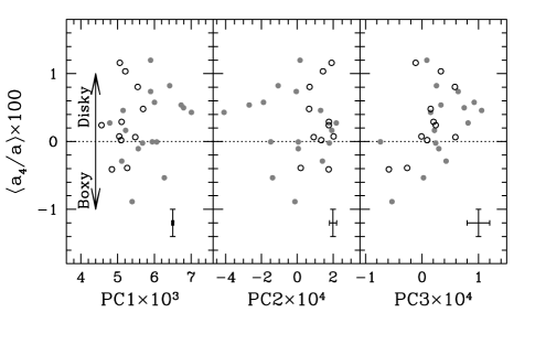
Figure 5: Comparison between the first three principal components and the structural parameter $a_{4}$ (see text for details). Characteristic error bars are shown.

5 Giving physical meaning to PCA

In order to relate this environmental segregation to actual differences in star formation history we need to project the principal components on to spectra corresponding to stellar populations whose ages and metallicities are known (Ronen et al. 1999; Madgwick et al. 2003). We generate two sets of models which describe the star formation history in terms of a single free parameter. These models give a distribution of stellar ages that is used to convolve simple stellar populations from the synthesis models of Bruzual & Charlot (2003). A Chabrier initial mass function (IMF) was used, although the result does not change significantly with respect to the choice of IMF. The composite SEDs are subsequently degraded to the instrumental resolution and velocity dispersion of a typical galaxy from our sample. The spectra are finally projected on to the basis vectors obtained by the application of PCA on the real data, and the results are shown in figures 7 and 8. The two sets of models assume a fixed metallicity and dust content, and describe the star formation rate in the following way:

1. EXP: Exponentially decaying star formation rate: SFR$(t)\propto\exp[-(t-t(z_{F}))/\tau_{\rm SF}]$. The process starts at a redshift $z_{F}=3$. The free parameter is the timescale ($\tau_{\rm SF}$), assumed to be in the range $0.1-5$ Gyr.

2. 2BURST: An old population is generated using an exponentially decaying star formation rate starting at $z_{F}=3$ with a timescale $\tau_{\rm SF}=0.5$ Gyr following the notation in (i). A second population is added with an age of 1 Gyr and the same metallicity as the old population. The free parameter is $f_{Y}$, which represents the stellar mass fraction in young stars.

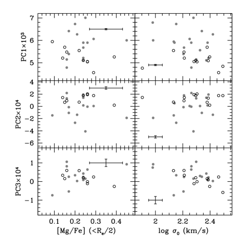
Figure 6: The first three principal components are compared with respect to the [Mg/Fe] abundance ratios measured within R${}_{e}/2$ (left) and the central velocity dispersion (right).

Figure 7 shows the (PC1,PC2) diagram obtained with the calibrated SEDs over a $\pm 200$Å spectral range that straddles the 4000Å break (top) and over a wider range of wavelengths ($3800-6000$Å ; bottom). The error bars are obtained by a Monte Carlo sampling of the SEDs. For each of the 100 realizations noise was added to each pixel according to the observed S/N. The error bars give the $1\sigma$ confidence levels. The lines are the projections of the models described above. The solid and dashed lines are dustless models with metallicity $2Z_{\odot}$ and $Z_{\odot}/2$, respectively, whereas the dotted line corresponds to solar metallicity and a dust reddening of E(B$-$V)$=0.2$ using the $R_{v}=3.1$ extinction model of Fitzpatrick (1999). The lines in the EXP models span a range of timescales $\tau_{\rm SF}=0.1-5$ Gyr. The stars (from the bottom left corner) correspond to $\tau_{\rm SF}=1,2,3$ and $4$ Gyr. The lines in the 2BURST models span a range of young stellar mass fractions $f_{Y}=0-0.2$, with the stars (from bottom-left corner) at $f_{Y}=\{0,0.05,0.01,0.15\}$.

Figure 8 shows the model prediction as a function of the free parameter, namely the star formation timescale in the EXP model (left) and the mass fraction in young stars for the 2BURST case (right). The same notation as in figure 7 applies to the solid, dotted and dashed lines. Instead of showing components PC1 and PC2 independently, we use a linear combination which captures the correlation between them. We rotate the (PC1,PC2) coordinate system so that one of the rotated axis follows the least squares fit to the data from panel a) in figure 2 (calibrated SEDs over $\Delta\lambda=3800-4200$Å ). Hence, we define:

$$\zeta\equiv 0.36{\rm PC1}-{\rm PC2}.$$ (4)

This method is analogous to the definition of the spectral parameter $\eta$ in Madgwick et al. (2002). However, in our paper the range of spectra is reduced to early-type galaxies, and we use information from the stellar continuum. Hence, we cannot establish a one-to-one correspondence between $\zeta$ and $\eta$.

For comparison, the histogram of the field and compact group samples are shown as a black and grey line, respectively. The model predictions are given as a function of $\zeta$. Our HCG sample features a wider distribution, including an important number of galaxies with values of $\zeta$ that corresponds to the presence of younger stars, either as a more extended SFH (in the EXP case) or as a higher value of $f_{Y}$ (2BURST model).

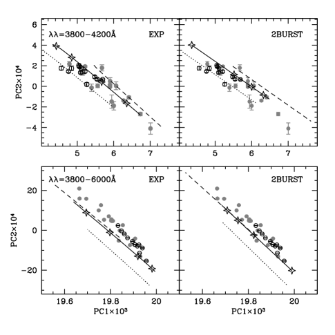
Figure 7: PCA and star formation histories (I): The top and bottom panels show PC1 and PC2 for the calibrated SEDs in the short (3800–4200Å ; top) and long (3800–6000Å ; bottom) wavelength range. The error bars are given for 100 realizations of the SED with the noise characteristics taken from the observations. The lines are projections of synthetic models at fixed metallicity, formed at $z_{F}=3$. The left panels (EXP model) span a range of exponentially decaying star formation timescales between $\tau_{\rm SF}=0.1$ and $5$ Gyr, whereas the panels on the right (2BURST model) fix $\tau_{\rm SF}=0.5$ Gyr and superimpose a young population of age 1 Gyr with a mass fraction $f_{Y}$ between $0$ and $0.2$. The solid and dashed lines correspond to dustless models with metallicity $2Z_{\odot}$ and $Z_{\odot}/2$, respectively. The dotted lines show the prediction for solar metallicity and E(B$-$V)$=0.2$ mag.

6 Discussion

In order to find environmental effects, compact groups are arguably the best places to look for recent phases of formation. Their moderate velocity dispersion and relatively high densities result in a fertile scenario for galaxy mergers. Recent work targeting the Fundamental Plane (de la Rosa, et al. 2001a) has not found significant differences with respect to early-type galaxies in the field. On the other hand, Proctor et al. (2004) used spectral indices to suggest that the ages of HCG galaxies were more similar to cluster galaxies. Environmental effects were not found between field and cluster galaxies by way of the Mg–$\sigma$ relation (Bernardi et al. 1998) or other kinematic and chemical signatures (Ziegler et al. 2005). The infamous age-metallicity degeneracy and the uncertainties underlying the translation from observed line strengths to actual abundance ratios prevent us from an accurate assessment of the difference in the star formation of early-type systems.

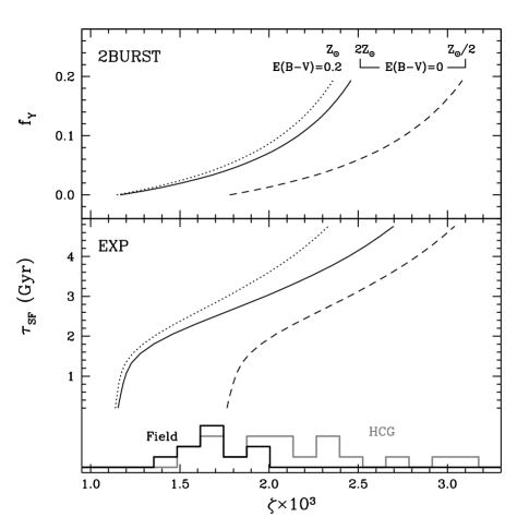
Figure 8: PCA and star formation histories (II): The histograms are the data measurements of group (grey) and field elliptical galaxies (black) according to parameter $\zeta=0.37PC1-PC2$ (see text for details). The curved lines are predictions according to the same two models described in figure 7. Notice that galaxies in Hickson groups have a wider range of $\zeta$, suggesting a larger range of stellar ages.

The data used in this paper comprises a consistent sample of elliptical galaxies in HCGs and in the field. The same telescope, instrument and configuration has been used in our galaxies. Hence, a model-independent approach such as principal component analysis is justified. The advantage of PCA over other techniques is that we maximise the information (in the sense of variance) extracted from the data without any reference to models. In this way we have found that no matter how we present the data to PCA – over a small range of wavelengths; without calibration; with continuum subtraction; selecting only the Lick/IDS spectral regions – we always find the same segregation between field and group samples. HCG elliptical galaxies span a wider range of principal components. This result, on its own, proves that early-type galaxies in compact groups have different star formation histories. Interestingly enough, more “traditional” observables such as the Fundamental Plane, structural parameters tracking the departure from elliptical isophotes, or [Mg/Fe] abundance ratios do not seem to be sensitive enough to these changes (see e.g. de la Rosa et al. (2001ab), Proctor et al. (2004) and Zepf & Withmore (1993). The segregation in (PC1,PC2) space is also found for the SEDs measured in different apertures, from $R_{e}/8$ out to $R_{e}$, implying that this effect does not have to do with radial gradients, but with a more global difference in the star formation histories.

Figures 5 and 6 explore the correlation of the PCs with other observables such as the structural parameter $a_{4}$ – which gives the diskyness/boxyness of the isophotes, velocity dispersion, or [Mg/Fe]. Remarkably, we find no correlation with either PC1 or PC2, but – within the limitations of our small sample – PC3 appears to be correlated with these “dynamically-related” observables.

The weakness of PCA is that it does not suggest any “physics” to explain this segregation. Figure 2 cleary shows that our field galaxies have similar star formation history, whereas HCG galaxies present a more complex distribution. In order to interpret these results, simple models spanning a range of ages and metallicities were generated and projected on the basis vectors given by the real data. Both models (an exponentially decaying star formation rate or a two-burst model) suggest younger ages for a fraction of the sample in HCGs. In contrast, the field sample is consistent with old stellar populations. Figure 8 implies that the wider distribution of the spectral parameter $\zeta$ in group galaxies is caused by a wider range of stellar ages. With respect to the correlation of PC3 with velocity dispersion or $a_{4}$, this component (see figure 1) has a feature around the magnesium absorption region. Hence, the correlations found tell us that higher velocity dispersions correspond to galaxies with metal-rich populations (i.e. the Mg–$\sigma$ relation, Bernardi et al. 1998) with boxy isophotes (Bender et al. 1989).

More work and larger samples are needed to exploit the full power of PCA, but the results we present here should illustrate both the complexity of extracting star formation histories from unresolved stellar populations and the potential of “non-traditional” statistical techniques towards the understanding of galaxy formation.

References

- (1) Bell, E. F., et al. 2004, ApJ, 608, 752
- (2) Bender, R., Döbereiner, S., Möllenhoff, C., 1988, A&A Suppl. Ser., 74, 385
- (3) Bender, R., Surma, P., Döbereiner, S., Möllenhoff, C., Madejsky, R., 1989, A&A, 217, 35
- (4) Bernardi M., Renzini A., da Costa L. N., Wegner G., Alonso M. V., Pellegrini P. S., Rité C., Willmer C. N. A. 1998, ApJ, 508, L143
- (5) Bernardi, M., et al. 2003, AJ, 125, 1882
- (6) Bruzual G., Charlot S., 2003, MNRAS, 344, 1000
- (7) Connolly, A. J., Szalay, A. S., Bershady, M. A., Kinney, A. L. & Calzetti, D., 1995, AJ, 110, 1071
- (8) Cowie, L. L., Songaila, A., Hu, E. M., Cohen, J. G., 1996, AJ, 112, 839
- (9) Coziol, R., Brinks, E. & Bravo-Alfaro, H., 2004, AJ, 128, 68
- (10) Davies, R. L., et al. 2001, ApJ, 548, L33
- (11) Deeming, T. J., 1964, MNRAS, 127, 493
- (12) de la Rosa, I. G., de Carvalho, R. R. & Zepf, S. E., 2001a, AJ, 122, 93
- (13) de la Rosa, I. G., Coziol, R., de Carvalho, R. R., Zepf, S. E., 2001b, Ap&SS, 276, 717
- (14) de Carvalho R. R., Djorgovski S., 1992, ApJ, 389, L49
- (15) de Carvalho, R. R., Gona̧lves, T. S., Iovino, A., Kohl-Moreira, J. L., Gal, R. R. & Djorgovski, S. G., 2005, AJ, 130, 425
- (16) Eisenstein, D. J., et al. 2003, ApJ, 585, 694
- (17) Ferreras, I. & Silk, J., 2003, MNRAS, 344, 455
- (18) Ferreras, I., Lisker, T., Carollo, C. M., Lilly, S. J. & Mobas her, B., 2005, ApJ, 635, 243
- (19) Fitzpatrick, E. L., 1999 PASP, 111, 63
- (20) Folkes, S. R., Lahav, O. & Maddox, S. J., 1996, MNRAS, 283, 651
- (21) Francis, P. J., Hewett, P. C., Foltz, C. B. & Chaffee, F. H., 1992 ApJ, 398, 476
- (22) Guzman R., Lucey J. R., Carter D., Terlevich R. J., 1992, MNRAS, 257, 187
- (23) Haynes M. P., 1989, clga.meet, 177
- (24) Hickson, P., 1982, ApJ, 255, 382
- (25) Hickson, P., 1994, Atlas Of Compact Groups Of Galaxies, Gordon and Breach Science Publishers S.A.
- (26) Iwamoto, K., Brachwitz, F., Nomoto, K., Kishimoto, N., Umeda, H., Hix, W. R., Thielemann, F.-K., 1999, ApJS, 125, 439
- (27) Jedrzejewski, R.I., 1987, MNRAS, 226, 747
- (28) Jesseit, R., Naab, Y., Burkert, A., 2005, MNRAS, 360, 1185
- (29) Khochfar, S., Burkert, A., 2005, MNRAS, 359, 1379
- (30) Lu, H., Zhou, H., Wang, J., Wang, T., Dong, X., Zhuang, Z., & Li, C., 2006, AJ, 131, 790
- (31) Matteucci, F. & Recchi, S., 2001, ApJ, 558, 351
- (32) McDermid, R. M., et al. 2005, New Ast. Rev., 49, 521
- (33) Madgwick, D. S., et al., 2002, MNRAS, 333, 133
- (34) Madgwick, D. S., Somerville, R., Lahav, O. & Ellis, R., 2003, MNRAS, 343, 871
- (35) Mendes de Oliveira, C., Coelho, P., González, J. J. & Barbuy, B., 2005, ApJ, 130, 55
- (36) Naim, A., Lahav, O., Sodre, L. Jr. & Storrie-Lombardi, M. C., 1995, MNRAS, 275, 567
- (37) Nolthenius, R. & White S. D. M., 1987, MNRAS, 225, 505
- (38) Pipino, A. & Matteucci, F., 2004, MNRAS, 347, 968
- (39) Proctor, R. N. Forbes, D. A., Hau, G. K.., Beasley, M. A., De Silva, G. M., Contreras, R. & Terlevich, A. I., 2004, MNRAS, 349, 1381
- (40) Proctor R. N., Forbes D. A., Forestell A., Gebhardt K., 2005, MNRAS, 362, 857
- (41) Ronen, S., Aragón-Salamanca, A. & Lahav, O., 1999, MNRAS, 303, 284
- (42) Rood H. J. & Struble, M. F., 1994, PASP, 106, 413
- (43) Rose J. A., Bower R. G., Caldwell N., Ellis R. S., Sharples R. M., Teague P., 1994, AJ, 108, 2054
- (44) Schlegel, D. J., Finkbeiner, D. P. & Davis, M., 1998, ApJ, 500, 525
- (45) Slonim, N., Somerville, R., Tishby, N., & Lahav, O., 2001, MNRAS, 323, 270
- (46) Tamura, N. & Ohta, K. 2000, AJ, 120, 533
- (47) Thomas, D., Maraston, C. & Bender, R., 2003, MNRAS, 339, 897
- (48) Trager, S. C., Worthey, G., Faber, S. M., Burstein, D. & González, J. J., 1998, ApJS, 116, 1
- (49) Trager S. C., Faber S. M., Worthey G., González J. J., 2000, AJ, 119, 1645
- (50) Treu, T., Ellis, R. S., Liao, T. X. & van Dokkum, P. G., 2005, ApJ, 622, L5
- (51) Yip, C. W., et al., 2004, 2004, AJ, 128, 2603
- (52) Zepf, S. E. & Whitmore, B. C., 1993, ApJ, 418, 72
- (53) Ziegler B. L., Thomas D., Böhm A., Bender R., Fritz A., Maraston C., 2005, A&A, 433, 519